Existence of naked singularities in Brans-Dicke theory of gravitation. An analytical and numerical study

Abstract

Within the framework of the scalar-tensor models of gravitation and by relying on analytical and numerical techniques, we establish the existence of a class of spherically symmetric spacetimes containing a naked singularity. Our result relies on and extends a work by Christodoulou on the existence of naked singularities for the Einstein-scalar field equations. We establish that a key parameter in Christodoulou’s construction couples to the Brans-Dicke field and becomes a dynamical variable, which enlarges and modifies the phase space of solutions. We recover analytically many properties first identified by Christodoulou, in particular the loss of regularity (especially at the center), and then investigate numerically the properties of these spacetimes.

1 Introduction

The issue of the validity of the (weak version of the) cosmic censorship conjecture remains one of the most important open problems in classical general relativity. Roughly speaking, it says that physically admissible solutions to the Einstein equations should not contain naked singularites, that is, all singularities formed in physically reasonable scenarios of gravitational collapse should be surrounded by event horizons and, hence, cannot send signals to far observers at future null infinity. A precise formulation of the conjecture can be found in [28, 9], together with the properties required on a solution to qualify as a physically “reasonable” process of singularity formation. These properties concern the smoothness and genericity of the initial conditions, and demand that the matter model undergoing collapse cannot form singularities of non-gravitational origin.

Even though the conjecture is still far from being proven in general, no definitive counter-example has been found so far, neither in numerical simulations nor in analytical investigations. An important step forward in this respect was the numerical analysis of the threshold for black hole formation. After the pioneering work of Choptuik [10] it has become clear that it is possible to form a naked singularity by fine-tuning (smooth) initial conditions toward the vicinity of the threshold of formation of arbitrarily small black holes. It turns out that the process is dynamically controlled by an unstable exact solution –referred to as a critical solution– which, itself, does contain a naked singularity. The fine-tuning is required to compensate for the instability of this solution and achieve a continuous approach to that solution. In that set-up, there is no dynamical formation of naked singularities and, therefore, this analysis does not provide a genuine counter-example to cosmic censorship. (See [22] for a review.)

In parallel to Choptuik’s work on the critical collapse of a real massless scalar field in spherical symmetry, Christodoulou [7] studied the Einstein-scalar field equations from a fully analytical point of view. In a truly remarkable series of papers about the global dynamics of solutions to this system, he constructed a family of exact solutions parametrized by some reals $k,a_{1}$ and showed that these spacetimes do contain a naked singularity in certain range of $a_{1}$, provided $0<k^{2}<1/3$. Later, in [8], he also established that these naked singularities are unstable under small perturbation. Christodoulou’s work provided the first complete mathematical proof of the formation of a naked singularity under gravitational collapse.

By construction, Christoudoulou’s spacetimes are homothetic, that is, continuously self-similar and, therefore, do not contain any privileged scale (such as a horizon of finite size), and so cannot contain a (finite) black hole. Consequently, these spacetimes are a priori good candidates to contain naked singularities with a central point of infinite curvature, denoted by $\mathcal{O}$; see [19]. The critical solution found by Choptuik also possesses self-similarity, but of a different type, known as discrete self-similarity. Since the symmetries are different, Christodoulou’s solutions cannot “relax” to the critical solution, and actually the relation between the two solutions is unclear —a problem that would deserve further study.

The parameter $k$, whose origin is in the massless scalar field (which only enters via its derivative in the Einstein equations), is essential in Christodoulou’s construction, as well as the key restriction

$$0<k^{2}<1/3.$$ (1.1)

Depending on the second parameter $a_{1}$, an apparent horizon (rather than a naked singularity) is also possible in this range of $k$. For

$$1/3\leq k^{2}<1$$ (1.2)

the future light-cone of $\mathcal{O}$ collapses to a line, which provides an example of a null singularity not preceded by an event horizon. For $k^{2}\geq 1$ the spacetimes are rather pathological (see [4] and the Carter-Penrose diagram in Figure 4 of [15]).

In all cases the parameter $k$ generates a mild loss of regularity at the center, which makes the curvature to be continuous but non-differentiable before the singularity at $\mathcal{O}$ is formed. This implies that the past light cone of $\mathcal{O}$ is non-regular, hence the initial conditions are not completely regular.

Note that, on the contrary, Choptuik’s critical solution is smooth everywhere except at the central singularity at $\mathcal{O}$ and, as a matter of fact, the sole requirements of regularity and discrete self-similarity select a unique solution, at least locally in the phase space; see [13, 14]. If the massless scalar field is taken to be complex then it is possible to construct a continuously self-similar solution which shares the regularity properties of the Choptuik spacetime, and also contains a naked singularity, but is not critical [17].

Our main objective in the present work is to investigate whether the relevance of $k$ and the role played by the limiting conditions on $k$ for the formation of naked singularities are “structurally stable”, that is, whether spacetimes with the same features can be constructed with extended models in which families of solutions with an equivalent parameter are present. Indeed, the model we consider contains Christodoulou’s model as a special case. Specifically, we work here within the scalar-tensor theory of gravitation and, especially, within the so-called Brans-Dicke theory.

The model under consideration here effectively adds an additional scalar field to Christodoulou’s system of equations, and makes $k$ a dynamical variable, denoted by $K$. Interestingly enough, our analysis leads to the same range in order to avoid the pathological behavior referred to above, namely

$$0<K_{*}^{2}<1,$$ (1.3)

where now $K_{*}$ is the value of the field $K$ at the past light cone of the singularity. We also show that, starting from an arbitrary initial value for $K$, the system under consideration dynamically evolves toward values $K$ below the threshold $1$. Therefore, the introduction of extra degrees of freedom allows to avoid the pathological spacetimes arising with the Einstein-scalar system.

Note that Liebling and Choptuik [21] have numerically shown the presence of critical phenomena in the Brans-Dicke system, the critical solution being discretely or continuously self-similar (depending a coupling constant). Again, being completely smooth, such a critical solution is not related to the solutions we construct in this article. For further results, see [5,18,20,26].

The system under study is significantly more involved than the one studied analytically by Christodoulou [7] and, although we do follow and generalize several important steps in the construction therein, we eventually must resort to numerical investigations to reach our final conclusions. In fact, by relying on numerics, we arrive at a better understanding of the class of solutions and are able to construct explicit examples.

An outline of this paper is as follows. In Section 2, we introduce the model of self-gravitating matter of interest, and we determine the general evolution equations under the assumption of radial symmetry. In Section 3, we impose the self-similar assumption and show that general solutions are parameterized by four functions of a single variable, denoted by $x$, which obey a system of ordinary differential equations (ODE). We construct solutions that are piecewise regular, with each piece separated by singular points across which careful matching is required. Specifically, in Sections 4 and 5, we successively construct the interior and exterior part of the past light-cone of the singularity. Finally, in Sections 6 and 7 we describe our numerical strategy and present various results and conclusions.

2 Scalar-tensor theories

2.1 Scalar-tensor gravity with scalar field

Scalar-tensor theories of gravity are alternative theories of gravity which are physically strongly motivated and have a long history in the literature. The fundamental assumption of these theories is that the gravitational field is mediated by one (or more) scalar field(s) in addition to the standard tensor field ($g_{\mu\nu}$) of Einstein’s general relativity. These theories satisfy the equivalence principle (since they are metric-based theories), but do not satisfy the strong version of the equivalence principle. The first theory of this kind was developed by Jordan [16], Fierz [12], and Brans and Dicke [6], and contains an additional parameter defining the coupling of the scalar field to the matter model. Later on, Bergmann [2], Nordtvedt [23], and Wagoner [27] extended this approach to a coupling via a function of the scalar field. Next, Damour and Esposito-Farèse [11] introduced a generalization based on an arbitrary number of scalar fields. More recently, cosmological models based on the so-called $f(R)$ gravity theories have attracted a lot of attention, which found applications in the study of relativistic stars [1]. These theories form a subclass of the scalar-tensor theories, and it is interesting to look for a better understanding of the corresponding spacetimes and, in particular as we do in the present work, to study the possible existence of spacetimes containing naked singularities.

Specifically, we are going to investigate a generalization of Christodoulou’s model when a a scalar field $\phi$ in coupled to a scalar-tensor theory of gravity for which the action reads (see [11, 25] for details):

$$S = S_{G}+S_{m}$$

$$= \frac{1}{4}\int_{M}\big{(}R-2g^{\mu\nu}\partial_{\mu}\psi\partial_{\nu}\psi\big{)}\,\sqrt{-g}\,\textrm{d}^{4}x-\frac{1}{2}\int_{M}\widetilde{g}^{\mu\nu}\partial_{\mu}\phi\partial_{\nu}\phi\,\sqrt{-\widetilde{g}}\,\textrm{d}^{4}x.$$

We use a system of units for the gravitational constant $G$ and the light speed $c$ such that $\frac{4\pi G}{c^{4}}=1$. The spacetime $M$ is four-dimensional and is endowed with two conformally-related metrics: the Einstein metric denoted by $g_{\mu\nu}$, and the Brans-Dicke (or physical) metric denoted by

$$\widetilde{g}_{\mu\nu}=a^{2}(\psi)g_{\mu\nu}.$$

In the latter, $a(\psi)>0$ is a coupling function entering the theory, and one recovers classical general relativity by choosing $a(\psi)$ to be constant.

This theory admits two scalar fields: one of them, $\phi$, represents the matter content of the spacetime and the other, $\psi$, generates the gravitational field. When $a$ is not just a constant, the matter field $\phi$ does interact with the physical metric $\widetilde{g}_{\mu\nu}$, whereas the gravitational field equations for $g_{\mu\nu},\psi$ are formulated in terms of $g_{\mu\nu}$, only.

2.2 Choice of coordinates

Throughout this paper we use a notation consistent with the one in Christodoulou [7], in order to make easier the comparison between the two models. We consider a general spherically symmetric spacetime whose metric is expressed in Bondi coordinates [3] as

$$g=-e^{2\nu}du^{2}-2e^{\nu+\lambda}dudr+r^{2}d\Omega^{2},$$

in which the metric coefficients $\lambda,\nu$ depend on the coordinates $u,r$, only, and $d\Omega^{2}$ represents the unit round metric on the 2-sphere. The relevant components of the Ricci tensor $R_{rr}$ and $R_{\theta\theta}$ are found to be (see for instance [3, 24]):

$$R_{rr}=\frac{2}{r}\left(\frac{\partial{\lambda}}{\partial{r}}+\frac{\partial{\nu}}{\partial{r}}\right),$$

$$R_{\theta\theta}=r\left(\frac{\partial{\lambda}}{\partial{r}}-\frac{\partial{\nu}}{\partial{r}}\right)e^{-2\lambda}+1-e^{-2\lambda},$$

with $R_{\varphi\varphi}=(\sin\theta)^{2}\,R_{\theta\theta}$. Observe that these formulas involve first-order derivatives of the metric coefficients, only. For completeness, we also determine the other two non-vanishing components of the Ricci tensor, which now involve second-order derivatives of the metric, i.e.

$$R_{uu}=e^{2(\nu-\lambda)}\left(\frac{2}{r}\frac{\partial{\nu}}{\partial{r}}-\frac{\partial{\lambda}}{\partial{r}}\frac{\partial{\nu}}{\partial{r}}+\left(\frac{\partial{\nu}}{\partial{r}}\right)^{2}+\frac{\partial{{}^{2}\nu}}{\partial{r^{2}}}\right)$$

$$\qquad\quad-e^{\nu-\lambda}\left(\frac{2}{r}\frac{\partial{\lambda}}{\partial{u}}+\frac{\partial^{2}{\nu}}{\partial{u}\partial{r}}+\frac{\partial^{2}{\lambda}}{\partial{u}\partial{r}}\right),$$

$$R_{ur}=e^{\nu-\lambda}\left(\frac{2}{r}\frac{\partial{\nu}}{\partial{r}}-\frac{\partial{\lambda}}{\partial{r}}\frac{\partial{\nu}}{\partial{r}}+\left(\frac{\partial{\nu}}{\partial{r}}\right)^{2}+\frac{\partial{{}^{2}\nu}}{\partial{r^{2}}}\right)-\frac{\partial^{2}{\nu}}{\partial{u}\partial{r}}-\frac{\partial^{2}{\lambda}}{\partial{u}\partial{r}}.$$

Note in passing the following simple relation:

$$e^{\lambda-\nu}R_{uu}-R_{ur}=-\frac{2}{r}\frac{\partial{\lambda}}{\partial{u}}.$$

Alternatively, one may consider the Einstein tensor $G_{\alpha\beta}=R_{\alpha\beta}-\frac{1}{2}R\,g_{\alpha\beta}$ for the metric $g_{\alpha\beta}$, and compute its essential components

$$G_{uu}=\frac{e^{2(\nu-\lambda)}}{r}\left(2\frac{\partial{\lambda}}{\partial{r}}+\frac{e^{2\lambda}-1}{r}-2e^{\lambda-\nu}\frac{\partial{\lambda}}{\partial{u}}\right),$$

$$G_{ur}=\frac{e^{(\nu-\lambda)}}{r}\left(\frac{e^{2\lambda}-1}{r}+2\frac{\partial{\lambda}}{\partial{r}}\right),$$

$$G_{rr}=\frac{2}{r}\left(\frac{\partial{\nu}}{\partial{r}}+\frac{\partial{\lambda}}{\partial{r}}\right).$$

2.3 Evolution equations

By varying the action of the theory with respect to both metrics, one gets two conformally-related stress-energy tensors $T^{\alpha\beta}$ and $\widetilde{T}^{\alpha\beta}=a^{-6}(\psi)T^{\alpha\beta}$. Denoting by $T=g_{\alpha\beta}T^{\alpha\beta}$ and $\widetilde{T}=\widetilde{g}_{\alpha\beta}\widetilde{T}^{\alpha\beta}$ their traces, one can check that (cf. [11] for details):

$$G_{\alpha\beta}=2T_{\alpha\beta}+2\left(\partial_{\alpha}\psi\partial_{\beta}\psi-\frac{1}{2}g_{\alpha\beta}g^{\mu\nu}\partial_{\mu}\psi\partial_{\nu}\psi\right)$$ (2.1)

and

$$\widetilde{T}_{\alpha\beta}={} \partial_{\alpha}\phi\,\partial_{\beta}\phi-\frac{1}{2}\,\widetilde{g}_{\alpha\beta}\,\widetilde{g}^{\rho\sigma}\partial_{\rho}\phi\,\partial_{\sigma}\phi,$$

$$T_{\alpha\beta}={} a^{2}(\psi)\widetilde{T}_{\alpha\beta}=a^{2}(\psi)\big{(}\partial_{\alpha}\phi\,\partial_{\beta}\phi-\frac{1}{2}g_{\alpha\beta}\,g^{\rho\sigma}\partial_{\rho}\phi\,\partial_{\sigma}\phi\big{)}.$$

Following Christodoulou [7], we use the future-directed null frame $(n,l)$, defined by

$$n=2e^{-\nu}\frac{\partial{}}{\partial{u}}-e^{-\lambda}\frac{\partial{}}{\partial{r}},$$

$$l=e^{-\lambda}\frac{\partial{}}{\partial{r}}.$$

By contraction of the Einstein equations (2.1) with $n,l$, we obtain the following system:

$$\frac{\partial{\lambda}}{\partial{r}}+\frac{\partial{\nu}}{\partial{r}} = r\left(\frac{\partial{\psi}}{\partial{r}}\right)^{2}+r\left(a(\psi)\frac{\partial{\phi}}{\partial{r}}\right)^{2},$$ (2.2)

$$\frac{\partial{\lambda}}{\partial{r}}-\frac{\partial{\nu}}{\partial{r}} = \frac{1-e^{2\lambda}}{r},$$ (2.3)

$$\qquad\frac{\partial{\lambda}}{\partial{u}} = r\left(\frac{\partial{\psi}}{\partial{r}}\frac{\partial{\psi}}{\partial{u}}-e^{(\lambda-\nu)}\left(\frac{\partial{\psi}}{\partial{u}}\right)^{2}\right)$$ (2.4)

$$+ra^{2}(\psi)\left(\frac{\partial{\phi}}{\partial{r}}\frac{\partial{\phi}}{\partial{u}}-e^{(\lambda-\nu)}\left(\frac{\partial{\phi}}{\partial{u}}\right)^{2}\right).$$

Note that these equations involve only first-order derivatives of the metric and scalar fields.

On the other hand, by defining the function

$$\sigma(\psi)={a^{\prime}(\psi)\over a(\psi)},$$ (2.5)

the evolution equation for the scalar field $\psi$ reads (cf. again [11])

$$\Box_{g}\psi=-\sigma(\psi)T=a^{\prime}(\psi)a(\psi)\,g^{\alpha\beta}\;\partial_{\alpha}\phi\;\partial_{\beta}\phi,$$

where $\Box_{g}$ is the wave operator associated with the Einstein metric. In our gauge, this equation is equivalent to

$$-2\left(\frac{\partial^{2}\psi}{\partial r\partial u}+\frac{1}{r}\frac{\partial{\psi}}{\partial{u}}\right)+e^{(\nu-\lambda)}\left(\frac{\partial^{2}\psi}{\partial r^{2}}+\frac{2}{r}\frac{\partial{\psi}}{\partial{r}}+\frac{\partial{(\nu-\lambda)}}{\partial{r}}\frac{\partial{\psi}}{\partial{r}}\right)$$

$$=a^{\prime}(\psi)a(\psi)\left(e^{(\nu-\lambda)}\left(\frac{\partial{\phi}}{\partial{r}}\right)^{2}-2\frac{\partial{\phi}}{\partial{r}}\frac{\partial{\phi}}{\partial{u}}\right).$$

Finally, the equation for the matter field $\phi$ is obtained from the zero-divergence law for the stress-energy tensor:

$$\widetilde{\nabla}_{\alpha}\widetilde{T}^{\alpha\beta}=0,$$

where $\widetilde{\nabla}$ is the covariant derivative associated with the physical metric. In terms of the Einstein metric, the zero-divergence law for the stress-energy tensor reads

$$\nabla_{\alpha}T^{\alpha\beta}={a^{\prime}(\psi)\over a(\psi)}T\,\nabla^{\beta}\psi,$$

where $\nabla$ denotes the covariant derivative for the metric $g$. This equation is equivalent to

$$\Box_{g}\phi=-{2a^{\prime}(\psi)\over a(\psi)}\,g^{\alpha\beta}\;\partial_{\alpha}\phi\;\partial_{\beta}\psi,$$

a linear equation for $\phi$ which, in our gauge, becomes

$$-2\left(\frac{\partial^{2}\phi}{\partial r\partial u}+\frac{1}{r}\frac{\partial{\phi}}{\partial{u}}\right)+e^{(\nu-\lambda)}\left(\frac{\partial^{2}\phi}{\partial r^{2}}+\frac{2}{r}\frac{\partial{\phi}}{\partial{r}}+\frac{\partial{(\nu-\lambda)}}{\partial{r}}\frac{\partial{\phi}}{\partial{r}}\right)$$

$$=-2\sigma(\psi)\left(e^{(\nu-\lambda)}\frac{\partial{\psi}}{\partial{r}}\frac{\partial{\phi}}{\partial{r}}-\frac{\partial{\phi}}{\partial{r}}\frac{\partial{\psi}}{\partial{u}}-\frac{\partial{\phi}}{\partial{u}}\frac{\partial{\psi}}{\partial{r}}\right).$$

2.4 Case of interest in this paper

For definiteness and simplicity, we study the case in which $\sigma(\psi)=\sigma$ is a constant, which corresponds to Brans-Dicke theory [6]. Integrating (2.5) we get

$$a(\psi)=a_{0}\,e^{\sigma\psi},$$

where $a_{0}$ is a dimensionless constant (independent of $\psi$). Assuming that it does not vanish, this constant can be eliminated by re-defining the matter field $\phi$, and so we end up with

$$a(\psi)=e^{\sigma\psi},$$

which is the choice made in the rest of this paper.

Our equations can be easily compared with those used in other investigations of the Brans-Dicke theory. For instance, Liebling and Choptuik [21] have (denoting their variables with subindex LC)

$$\phi=\psi_{LC},\qquad\sigma\psi=-\frac{1}{2}\xi_{LC},\qquad 2\sigma^{2}=(4\pi)\lambda_{LC},$$

which imply $a^{2}=e^{-\xi_{LC}}$. (Special care must be taken with the fact that, in [21], units with $G=c=1$ are used so that various factors like $4\pi$ arise in their equations.)

3 Self-similar assumption and the reduced system

3.1 Essential field equations

We now impose continuous self-similarity on the solutions, that is,

$${\cal L}_{S}g_{\mu\nu}=2g_{\mu\nu}$$ (3.1)

for some (conformal) homothetic Killing field denoted by $S^{\mu}$. To work with self-similar solutions, it is convenient to use adapted coordinates, in which the integral lines of $S^{\mu}$ are now coordinate lines. Every spherically symmetric and self-similar spacetime (except Minkowski) has a singularity at a point on the central world-line, and we shall use it to define the origin of time, so that $u=0$ represents the future null cone of the singularity. Moreover, since we are interested in the process of the formation of singularities, we (principally) work in the past region $u<0$.

We define Bondi’s self-similar coordinates by

$$x=\frac{r}{-u},\qquad\tau=-\log(-u),$$ (3.2)

where the sign in $\tau$ is chosen so that $u$ and $\tau$ increase simultaneously toward the future. The homothetic vector is now $S=-\partial_{\tau}$, with integral lines $x=$const., and points away from the singularity —which is now located at $\tau=+\infty$. Referring for instance [15] for the general geometry of self-similar spacetimes, we note that in these coordinates the metric reads

$$g=e^{-2\tau}\left((-e^{2\nu}+2xe^{\nu+\lambda})d\tau^{2}-2e^{\nu+\lambda}d\tau dx+x^{2}d\Omega^{2}\right),$$ (3.3)

where $\nu$ and $\lambda$ are functions of $(\tau,x)$. The Lie derivative ${\cal L}_{S}$ is now simply $-\partial/\partial\tau$ and, consequently, the symmetry condition (3.1) implies that all metric coefficients depend on $x$, only, so

$$\nu=\nu(x),\quad\qquad\lambda=\lambda(x).$$

This implies similar conditions on the scalar fields and, since $\psi$ arises in an undifferentiated form, the relevant condition is

$$\frac{\partial}{\partial\tau}\psi=0,\quad\mbox{ implying }\quad\psi=\psi(x).$$

However, $\phi$ only enters the equations in differentiated form and hence the condition is

$$\frac{\partial}{\partial\tau}\partial_{\mu}\phi=0,\quad\mbox{ implying }\quad\phi=\chi(x)+k\tau,$$

where $\chi=\chi(x)$ is a function of $x$, only, and $k$ is a dimensionless real constant.

Remark. An interesting variant of the above symmetry assumption was adopted in [17], where self-similar, complex-valued, scalar field solutions are constructed from the ansatz $e^{i\omega\tau}\xi(x)$, for some dimensionless real constant $\omega$.

Following Christodoulou [7], we define

$$\beta =1-\frac{e^{\nu-\lambda}}{2x},$$

$$\theta =x\chi^{\prime}(x),$$ (3.4)

$$\xi =x\psi^{\prime}(x),$$

and we emphasize that $\beta$ will replace $\nu$ from now on. The Einstein equation (2.3) becomes

$$x\frac{d\beta}{dx}=(1-\beta)(2-e^{2\lambda})$$

and, by adding (2.2) and (2.3) together, we find

$$2x\,\frac{d\lambda}{dx}=\xi^{2}+e^{2\sigma\psi}\theta^{2}-(e^{2\lambda}-1).$$ (3.5)

The third Einstein equation (in combination with the other two equations) yields the constraint equation

$$e^{2\lambda}=1+k^{2}\,e^{2\sigma\psi}+\frac{\beta}{1-\beta}\left((\theta+k)^{2}e^{2\sigma\psi}+\xi^{2}\right).$$ (3.6)

Moreover, the wave equation for the matter field reads

$$\beta x\frac{d\theta}{dx}+\left(1-(1-\beta)e^{2\lambda}\right)\,\theta+k=-\sigma(k+2\beta\theta)\xi,$$ (3.7)

and the wave equation for the Brans-Dicke field is

$$\beta x\frac{d\xi}{dx}+\big{(}1-(1-\beta)e^{2\lambda}\big{)}\,\xi=\sigma e^{2\sigma\psi}(k+\beta\theta)\theta.$$ (3.8)

(We emphasize that there is no factor $2$ in the parenthesis of the right-hand side of this last equation.)

In conclusion, using the constraint (3.6) to eliminate $\lambda$, we arrive at a system of four ordinary differential equations:

$$x\frac{d\beta}{dx} =1-k^{2}e^{2\sigma\psi}-\big{(}e^{2\sigma\psi}(\theta+2k)\theta+\xi^{2}+1\big{)}\,\beta,$$ (3.9)

$$\beta x\frac{d\theta}{dx} =k(ke^{2\sigma\psi}\theta-1)-\sigma(k+2\beta\theta)\xi+\big{(}e^{2\sigma\psi}(\theta+2k)\theta+\xi^{2}-1\big{)}\,\beta\theta,$$

$$\beta x\frac{d\xi}{dx} =k^{2}e^{2\sigma\psi}\xi+\sigma e^{2\sigma\psi}(k+\beta\theta)\theta+\big{(}e^{2\sigma\psi}(\theta+2k)\theta+\xi^{2}-1\big{)}\,\beta\xi,$$

$$x\frac{d\psi}{dx} =\xi.$$

The first two equations above reduce to Christodoulou’s equations (see (0.27a) and (0.27b) therein) provided $\sigma$ and $\xi$ vanish identically. Note that we can simultaneously change the signs of $\theta$ and $k$ without changing the structure of the system. Hence, without loss of generality, we can assume that $k\geq 0$, while $\theta$ still can have any sign.

3.2 Reduced system

We have found it convenient to rescale $\theta$ with an exponential factor $e^{\sigma\psi}$, which compensates for the discrepancy by a factor $2$ between equations (3.7) and (3.8) (as pointed out earlier). We define

$$\Theta=e^{\sigma\psi}\theta,$$

and the remaining exponential terms can be combined with $k$ into a single variable:

$$K=e^{\sigma\psi}k.$$

The notation is intended to compare with Christodoulou’s case, for which $\Theta$ and $K$ coincide with $\theta$ and $k$, respectively. Using the variable $s=\ln x$ and denoting $d/ds$ as a prime, the system (3.9) now reads

$$\beta^{\prime} =1-K^{2}-\big{(}2K\Theta+\Theta^{2}+\xi^{2}+1\big{)}\,\beta,$$

$$\beta\,\Theta^{\prime} =K\big{(}K\Theta-1\big{)}-\sigma\big{(}K+\beta\Theta\big{)}\,\xi+\big{(}2K\Theta+\Theta^{2}+\xi^{2}-1\big{)}\,\beta\Theta,$$ (3.10)

$$\beta\,\xi^{\prime} =K^{2}\xi+\sigma\big{(}K+\beta\Theta\big{)}\,\Theta+\big{(}2K\Theta+\Theta^{2}+\xi^{2}-1\big{)}\,\beta\xi,$$

$$K^{\prime} =\sigma K\xi.$$

It is also convenient to make the change of variable

$$\alpha=\frac{1}{\beta},$$

such that the system under consideration becomes polynomial in all variables:

$$\alpha^{\prime} =\big{(}\alpha K^{2}+2K\Theta+\Theta^{2}+\xi^{2}+1\big{)}\,\alpha-\alpha^{2},$$

$$\Theta^{\prime} =\big{(}\alpha K^{2}+2K\Theta+\Theta^{2}+\xi^{2}-1\big{)}\,\Theta-\sigma(\alpha K+\Theta)\xi-\alpha K,$$ (3.11)

$$\xi^{\prime} =\big{(}\alpha K^{2}+2K\Theta+\Theta^{2}+\xi^{2}-1\big{)}\,\xi+\sigma(\alpha K+\Theta)\Theta,$$

$$K^{\prime} =\sigma K\xi.$$

From now on, we refer to these equations as the reduced system, which is our main object of study. We sometimes use it in the form (3.2), evolving $\beta$ instead of $\alpha$.

Observe the combination

$$\alpha K^{2}+2K\Theta+\Theta^{2}+\xi^{2}=(\alpha-1)(e^{2\lambda}-1).$$ (3.12)

We will later use the variable

$$L=\sqrt{\Theta^{2}+\xi^{2}},$$

that obeys the evolution equation

$$\frac{1}{2}(L^{2})^{\prime}=\big{(}\alpha K^{2}+2K\Theta+L^{2}-1\big{)}\,L^{2}-\alpha K\Theta.$$ (3.13)

Remark. From $\Theta$ and $\xi$ one can form a complex function $\Lambda=\Theta+i\xi$, with norm $|\Lambda|=L$, which satisfies the differential equation

$$\Lambda^{\prime}=\alpha\left(Z_{1}-Z_{0}\right)\left(Z_{0}\Lambda-1\right)+\left|\Lambda\right|\left(\Lambda+\frac{Z_{1}}{2}\right)+\frac{\Lambda^{2}Z_{1}}{2}-\Lambda$$

with $Z_{0}=K+i\sigma$ and $Z_{1}=2K+i\sigma$.

4 Interior solution originating at the center

4.1 Analytical strategy

The construction of our spacetimes, as solutions of the reduced system (3.2), will be performed in several steps; a main difficulty stems from the fact that the equations become singular for several values of the $x$-coordinate. This happens at the center of spherical symmetry, $x=0$, and at the self-similarity horizons corresponding to those values of $x$ for which the homothetic vector $S$ becomes null. In our Bondi coordinates, this corresponds to the condition $g(\partial_{\tau},\partial_{\tau})=g_{\tau\tau}=0$ for the past light-cone, which reads (see (3.3))

$$-e^{2\nu}+2xe^{\nu+\lambda}=0,\qquad\textrm{or}\quad\beta=0.$$

This section describes the construction of the past of the singularity, namely the region between the center worldline and the past lightcone of the singularity, the first self-similarity horizon. Following Christodoulou, we shall refer to this region as the interior solution.

\psfrag{Interior}{Interior}\psfrag{Exterior}{Exterior}\psfrag{Future}{Future}\psfrag{x=0}{$\!\!\!\!\!\!x=0$}\psfrag{x=x*}{$x=x_{*}$}\psfrag{x=inf}{$\!\!x=+\infty$}\includegraphics[width=142.26378pt]{Figures/patches.eps}

Figure 1: Schematic representation of the different regions in which the the solution is divided, matching at the past light-cone ($x=x_{*}$) and the future light-cone ($x=+\infty$). The dashed lines denote Bondi coordinate lines.

4.2 Critical points and regularity at the center

We begin by determining all critical points corresponding to equilibria of the reduced system, provided $\sigma\not=0$. In view of the right-hand side of (3.2) and provided the unknown functions $\alpha,\Theta,\xi,K$ have vanishing derivatives, only the following alternatives can arise:

• $\alpha=0$, $\Theta=0$, $\xi=0$, $K$ arbitrary,

• $\alpha=1$, $\Theta=-K$, $\xi=0$, $K$ arbitrary,

• $\alpha=0$, $\Theta=0$, $\xi^{2}=1$, $K=0$,

• $\alpha=2$, $\Theta=0$, $\xi^{2}=1$, $K=0$.

Points (c) actually belong to the exact solutions $\alpha=0,\Theta=0,\xi=\pm 1,K=K_{0}e^{\pm\sigma s}$. Note that this collection of fixed points is not an extension of Christodoulou’s result. This is due to the fact that the condition $\xi=0$ is not preserved by the evolution. In fact, several fixed points in Christodoulou’s problem are no longer fixed in our case. This is clear in Figure 2, which shows a projection of the evolution flow on a slice $(\Theta,\xi)$ of phase space.

\psfrag{theta}{$\Theta$}\psfrag{xi}{$\xi$}\includegraphics[width=227.62204pt]{Figures/slicethetaxi.eps}

Figure 2: Projection onto the plane ($\alpha=0$, $\Theta$, $\xi$, $K=1/2$) of streamlines of the flow vector field of system (3.2) for $\sigma=1/3$. We have marked the fixed point (a) at $\Theta=0,\xi=0$ and the projections at $\Theta=0,\xi=\pm 1$ of the exact solutions mentioned in the text. We have also marked the points $\Theta=-K\pm\sqrt{K^{2}+1}$, which are fixed points in Christodoulou’s system, but are no longer fixed points in our system. Those four points now form part of an unstable projected structure that resembles a limit circle, though we do not know whether a true limit cycle exists in the full phase space.

The center of symmetry must correspond to one of the above cases. We need to rely on physically motivated regularity requirements, to select one of them. Specifically, we impose that the center of symmetry is regular before the formation of the singularity. Recall that the Hawking mass is determined from the metric coefficient $\lambda$ by the relation

$$1-\frac{2m}{r}=e^{-2\lambda}.$$ (4.1)

In order to avoid a singular behavior at the center, we impose that the mass tends to zero, which implies $\lambda=0$ at the center. The equation (3.12) then selects the fixed points (a) and (b), above.

Regularity at the center also requires that $\nu(x=0)$ is finite, to avoid a coordinate time singularity. However, the value of $\nu$ at the center is gauge-dependent and, by normalizing $\nu$ to vanish at the center, the coordinate time $u$ in (3.2) coincides with the proper time of the central observer. Consequently, $\beta$ in (3.1) behaves like $\beta\sim-1/(2x)$ and, equivalently $\alpha\sim-2x$ at the center. In particular, this condition implies that $\alpha=0$ at the center, which is consistent with the critical point (a) above, only.

In summary, we obtain the following values for the critical point of interest:

$$\alpha=0,\quad\Theta=0,\quad K=K_{0},\quad\xi=0\qquad\textrm{ at the center }x=0,$$ (4.2)

where $K_{0}$ is an arbitrary non-negative constant.

4.3 Linear stability of the critical point at the center

After linearizing around the critical point (a), the Jacobian matrix of the system in the linearized variables $(\delta\alpha,\delta\Theta,\delta\xi,\delta K)$ reads

$$\left(\begin{array}[]{cccc}1&0&0&0\\ -K_{0}&-1&0&0\\ 0&0&-1&0\\ 0&0&\sigma K_{0}&0\end{array}\right).$$

Its eigenvalues are $1,-1,-1,0$, with respective eigenvectors

$$e^{(1)}=\left(\begin{array}[]{c}1\\ -K_{0}/2\\ 0\\ 0\end{array}\right),\quad e^{(2)}=\left(\begin{array}[]{c}0\\ 1\\ 0\\ 0\end{array}\right),\quad$$

$$e^{(3)}=\left(\begin{array}[]{c}0\\ 0\\ 1\\ -\sigma k\end{array}\right),\quad e^{(4)}=\left(\begin{array}[]{c}0\\ 0\\ 0\\ 1\end{array}\right),$$

respectively. (Figure 2 corresponds to the two negative eigenvalues.) The origin (a), therefore, has an unstable branch, tangent to the vector $e^{(1)}$, and the corresponding solutions in the neighborhood of (a) have the form

$$\left(\begin{array}[]{c}\alpha\\ \Theta\\ \xi\\ K\end{array}\right)=\left(\begin{array}[]{c}0\\ 0\\ 0\\ K_{0}\end{array}\right)+a_{1}\,e^{s}\left(\begin{array}[]{c}1\\ -K_{0}/2\\ 0\\ 0\end{array}\right)+o(e^{s}),$$

where $a_{1}$ is a parameter.

Imposing the normalization $\alpha\,x^{-1}\to-2$ at (a), we get $a_{1}=-2$ and we obtain an interior solution in the neighborhood of the center, satisfying

$$\left(\begin{array}[]{c}\alpha\\ \Theta\\ \xi\\ K\end{array}\right)=\left(\begin{array}[]{c}-2e^{s}\\ K_{0}e^{s}\\ 0\\ K_{0}\end{array}\right)+o(e^{s}).$$ (4.3)

We now show that this implies that the spacetime is (mildly) singular at the center. We start by taking the trace of (2.1), which gives the Ricci scalar

$$R=-2T+2\left(g^{\alpha\beta}\partial_{\alpha}\psi\partial_{\beta}\psi\right).$$ (4.4)

Taking the form (3.3) of the metric, we get

$$R = 2e^{2\tau}\left(-2e^{-(\nu+\lambda)}\left(a^{2}\partial_{\tau}\phi\partial_{x}\phi+\partial_{\tau}\psi\partial_{x}\psi\right)\right.$$

$$\left.+\left(e^{-2\lambda}-2xe^{-(\nu+\lambda)}\right)\left(a^{2}\left(\partial_{x}\phi\right)^{2}+\left(\partial_{x}\psi\right)^{2}\right)\right)$$

$$= -\frac{2e^{2\tau}\left(\Theta K+\beta\left(\Theta^{2}+\xi^{2}\right)\right)}{x^{2}\left(2\beta\Theta K+K^{2}+\beta\left(\Theta^{2}+\xi^{2}-1\right)+1\right)}.$$ (4.6)

Using the reduced system (3.2) together with the expansion (4.3), we get (for the first two variables)

$$\alpha ={}-2\,e^{s}-4e^{2s}+o\left(e^{2s}\right),$$

$$\Theta ={}K_{0}\,e^{s}+\frac{4K_{0}}{3}\,e^{2s}+o\left(e^{2s}\right).$$

Therefore, the local expression for the Ricci scalar becomes (we have replaced $e^{s}$ with $x$)

$$R=e^{2\tau}\left(-2K_{0}^{2}-4K_{0}^{2}x+o\left(x^{2}\right)\right),$$ (4.7)

where we have used $\lim_{x\to 0}\nu(x)=\lim_{x\to 0}\lambda(x)=0.$

Consequently, the presence of a non-vanishing linear term $-4K_{0}^{2}x$ in (4.7) shows that, when viewed as a geometric object in a spherically symmetric spacetime, the scalar curvature $R$ is continuous but not differentiable at the center $x=0$. (Only even powers of $x$ should, otherwise, be allowed.) Hence, the spacetime contains a (mild) singularity before the central curvature singularity forms at $u=0$.

4.4 Integration in the interior region

We denote by $(-\infty,s_{*})$ the maximal interval on which the solution is defined, and now check that, provided $s_{*}$ is finite, $\alpha$ must blow-up.

Claim 1. Either the solution is defined and regular up to $s_{*}=+\infty$, or else $\alpha(s)\to-\infty$ but $\Theta,\xi$ and $K$ remain bounded as $s\to s_{*}$.

Indeed, se suppose that $s_{*}$ is finite and we are going to prove that both $\Theta$ and $\xi$ are bounded. First, $\alpha<0$ for all $s<s_{*}$. Indeed, $\alpha(s)<0$ at least for an interval of the form $(-\infty,s_{0}]$ with $s_{0}<s_{*}$. Thus, $\beta(s)=1/\alpha(s)$ is negative and finite on the same interval. Also, setting $B=2K\Theta+\Theta^{2}+\xi^{2}+1$ and $C=1-K^{2}$, from the first equation of (3.2) we deduce that (for $s_{0}\leq s<s_{*}$)

$$\beta(s)=\beta(s_{0})e^{-\int_{s_{0}}^{s}B(u)du}+\int_{s_{0}}^{s}C(u)e^{-\int_{u}^{s}B(t)dt}du.$$

Thus, $\beta(s)$ remains finite on $(-\infty,s_{*})$ so that $\alpha(s)=1/\beta(s)$ can not vanish in this interval and remains negative. Now, the equation (3.5) reads

$$2\lambda^{\prime} =(\xi^{2}+\Theta^{2}\big{)}-(e^{2\lambda}-1)$$

$$=L^{2}-(e^{2\lambda}-1),$$

thus we have

$$e^{2\lambda}={{e^{s}g(s)}\over{\int_{-\infty}^{s}e^{s^{\prime}}g(s^{\prime})\,ds^{\prime}}},\qquad g(s)=e^{\int_{-\infty}^{s}L^{2}(s^{\prime})\,ds^{\prime}}.$$

But, $L$ can not vanish, except at an isolated point. Indeed, if there is $s_{1}<s_{*}$ such that $L(s_{1})=0$, then $\Theta(s_{1})=0$ with $\Theta^{\prime}(s_{1})=-\alpha(s_{1})K(s_{1})>0$. Thus, functions $\Theta$ and $L$ are both different from zero in the neighborhood of $s_{1}$. We obtain that the function $g$ is strictly monotone increasing,

$$\int_{-\infty}^{s}e^{s^{\prime}}g(s^{\prime})\,ds^{\prime}<g(s)\int_{-\infty}^{s}e^{s^{\prime}}\,ds^{\prime}=e^{s}g(s),$$

so that $e^{2\lambda}>1$, i.e., $\lambda(s)>0$ for all $s<s_{*}$. Setting

$$\Gamma=\alpha K^{2}+2\Theta K+L^{2},$$

and using (3.6), we obtain

$$e^{2\lambda}-1={\Gamma\over{\alpha-1}}.$$

Since $\alpha<0$ for $s<s_{*}$, we get $\Gamma(s)<0$ for all $s\in(-\infty,s_{*})$.

Let us introduce now the quantity

$$H=\Theta^{2}+\xi^{2}+2{\xi\over\sigma}=L^{2}+2{\xi\over\sigma}.$$

Using (3.13) and the third equation in (3.2), we obtain

$$H^{\prime}=\Gamma H+\Gamma L^{2}-2(\xi^{2}+{\xi\over\sigma}).$$

Then, completing the square in the last term,

$$H^{\prime}\leq\Gamma H+{1\over 2\sigma^{2}}.$$

Now, fix $s_{0}<s_{*}$. Using the Gronwall inequality, we get for $s\in[s_{0},s_{*})$,

$$H(s)\leq H(s_{0})e^{\int_{s_{0}}^{s}\Gamma(u)du}+{1\over{2\sigma^{2}}}\int_{s_{0}}^{s}e^{\int_{u}^{s}\Gamma(t)dt}du$$

$$\leq H^{+}(s_{0})+{1\over{2\sigma^{2}}}(s-s_{0})\leq H^{+}(s_{0})+{1\over{2\sigma^{2}}}(s_{*}-s_{0}),$$

where $H^{+}(s_{0})={\rm max}(0,H(s_{0}))$. We deduce that both $\Theta$ and $\xi$ are bounded, and since $K(s)=K(s_{0})e^{\int_{s_{0}}^{s}\xi}$, $K$ is also bounded. We conclude that necessarily $\alpha\to-\infty$, as $s\to s_{*}$.

Claim 2. Assume that $s_{*}<+\infty$. Then, there exists a real $0<K_{*}<1$ such that,

$$\lim_{s\to s_{*}}K(s) ={}K_{*},$$

$$\lim_{s\to s_{*}}\Theta(s) ={}\frac{K_{*}}{K_{*}^{2}+\sigma^{2}},$$

$$\lim_{s\to s_{*}}\xi(s) ={}-\frac{\sigma}{K_{*}^{2}+\sigma^{2}}.$$

To establish this claim, we proceed as follows. First, since $\xi$ remains bounded, $\int_{-\infty}^{s_{*}}\xi(s)ds=\Xi$, where $\Xi$ is some real constant, so that

$$\lim_{s\to s_{*}}K(s)=K_{0}e^{\sigma\,\Xi}=K_{*},$$

with $K_{*}>0$. Also, the first equation of (3.2) gives $\beta^{\prime}(s)\to 1-K_{*}^{2},$ and we obtain

$$\frac{\beta(s)}{s_{*}-s}\to K_{*}^{2}-1.$$ (4.8)

But since $\beta(s)<0$ for $s<s_{*}$, we get that necessarily $K_{*}\leq 1$. The case $K_{*}=1$ will be excluded at the end of the argument.

Now, let us introduce the new variables

$$\delta_{1}=K\Theta-\sigma\xi-1,\,\,\,\,\,\,\delta_{2}=K\xi+\sigma\Theta.$$ (4.9)

Thus, the expressions of $\Theta^{\prime}$ and $\xi^{\prime}$ in (3.2) become

$$\Theta^{\prime}={K\over\beta}\delta_{1}+h_{1},\,\,\,\,\,\xi^{\prime}={K\over\beta}\delta_{2}+h_{2},$$ (4.10)

where

$$h_{1}=(2K\Theta+\Theta^{2}+\xi^{2}-1)\Theta-\sigma\xi\Theta,\$$

$$h_{2}=(2K\Theta+\Theta^{2}+\xi^{2}-1)\xi+\sigma\Theta^{2}.$$

Using (4.9), (4.10) and the last equation in (3.2), we get

$$\delta_{1}^{\prime}={K\over\beta}(K\delta_{1}-\sigma\delta_{2})+l_{1},\,\,\,\,\delta_{2}^{\prime}={K\over\beta}(\sigma\delta_{1}+K\delta_{2})+l_{2},$$ (4.11)

where

$$l_{1} =\sigma K\xi\Theta+Kh_{1}-\sigma h_{2},$$ (4.12)

$$l_{2} =\sigma K\xi^{2}+Kh_{2}+\sigma h_{1}.$$ (4.13)

Thanks to (4.11), the quantity $\delta=(\delta_{1}^{2}+\delta_{2}^{2})^{1/2}$ satisfies

$$\delta^{\prime}={K^{2}\over\beta}\delta+l,$$ (4.14)

where

$$l=\frac{l_{1}\delta_{1}+l_{2}\delta_{2}}{\delta}.$$

By assumption, $l_{1}$ and $l_{2}$ are bounded on $(-\infty,s_{*})$ so that $l$ is bounded too. Choosing $s<s_{*}$, and integrating (4.14) over $[s_{0},s]$ we obtain

$$\delta(s)=e^{-\zeta(s)}\Big{(}\delta(s_{0})+\int_{s_{0}}^{s}e^{\zeta(s^{\prime})}\,l(s^{\prime})ds^{\prime}\Big{)},$$

where

$$\zeta(s)=-\int_{s_{0}}^{s}\frac{K^{2}(s^{\prime})}{\beta(s^{\prime})}ds^{\prime}.$$

Function $\zeta$ is increasing, and by (4.8), it tends to $+\infty$ as $s\to s_{*}$, together with its derivative $\zeta^{\prime}$. Thus,

$$e^{-\zeta(s)}\int_{s_{0}}^{s}e^{\zeta(s^{\prime})}ds^{\prime}\to 0\,\,as\,\,s\to s_{*},$$

and since $l$ is bounded we obtain

$$\lim_{s\to s_{*}}\delta(s)=0.$$

Finally, we can rewrite (4.9) in the form

$$\Theta={1\over\sigma^{2}+K^{2}}(K(\delta_{1}+1)+\sigma\delta_{2}),\qquad\qquad\xi={1\over\sigma^{2}+K^{2}}(-\sigma(\delta_{1}+1)+K\delta_{2}),$$

and we get

$$\lim_{s\to s_{*}}\Theta(s)=\frac{K_{*}}{K_{*}^{2}+\sigma^{2}},\qquad\qquad\lim_{s\to s_{*}}\xi(s)=-\frac{\sigma}{K_{*}^{2}+\sigma^{2}}.$$

Now, it remains to prove that $K_{*}<1$, i.e., $K_{*}=1$ is excluded when $s_{*}<+\infty$, as well as $K_{*}>1$. So, assume by contradiction that $K_{*}=1$. Thus, the last equation in (3.2) reads

$$K(s)=1-\frac{\sigma^{2}}{\sigma^{2}+1}(s-s_{*})+o(|s-s_{*}|),$$ (4.15)

Also, (3.2) gives $\beta^{\prime}(s)\to 0$ as $s\to s_{*}$, so that $\beta(s)=o(|s_{*}-s|)$. More precisely, using (4.15) in the first equation of (3.2) we obtain the following expansion

$$\beta^{\prime}(s)=2\frac{\sigma^{2}}{\sigma^{2}+1}(s-s_{*})+o(|s-s_{*}|).$$

Thus, $\beta$ is decreasing in the neighborhood of $s_{*}$ which is impossible since $\beta<0$ and $\beta(s)\to 0$ as $s\to s_{*}$.

4.5 Conclusions for the interior region

In the interior region, the situation is similar to that of Christodoulou, in the sense that the presence of a first self-similarity horizon, the past light-cone of the singularity, is determined by the value of a constant $K_{*}$, which must be below the threshold $1$. The main difference is that in Christodoulou’s case this constant is the parameter $k$, fixed throughout the problem, while in our case the constant $K_{*}$ is dynamically determined by the evolution and, so, depends on the set of initial conditions, especially the initial value $K_{0}$ of the variable $K$.

We have performed numerical integrations of the reduced system of equations to investigate how $K$ evolves. The results are summarized in Figure 3, which shows several evolutions of $K$ starting from different values at the center. In all cases we see a decrease of $K$ until values below $1$ are reached, and then we reach the singular point $x_{*}=e^{s_{*}}$, where the integration is stopped. We have found this behavior in all tested cases, including cases with large values of the initial $K_{0}$ (above 1000, say). The value of $\sigma$ does not alter the qualitative picture, though the decay of $K$ is faster for larger values of $\sigma$. Interestingly enough, for large values of $K_{0}$ the final value $K_{*}$ is almost independent of that initial value. For sufficiently large values of $\sigma$ we find numerically that $K_{*}$ tends to $4/(3\sigma)$.

In other words, we can have solutions in which the central singularity has a past light-cone for initial values of the constant $k$ for which Christodoulou’s corresponding solution would be more pathological, with that light-cone becoming actually a border of the spacetime.

\psfrag{coordx}{$x$}\psfrag{KK}{$K$}\includegraphics[width=284.52756pt]{Figures/Kinterior.eps}

Figure 3: Evolution of $K(x)$ starting from values $K_{0}$ ranging from $0$ to $7$ in steps $1/2$, hence $15$ curves. The coupling constant is $\sigma=3/2$ in all cases. Each evolution stops when reaching the singular point $x_{*}$, which for $K_{0}=0$ corresponds to Minkowski, with $x_{*}=1/2$. For reference, a dashed line represents the value $K=1$.

5 Extension to the exterior region

5.1 The singular points

According to the previous section when $s_{*}<+\infty$, the solution of (3.2) converges to a singular point of the form $(\beta,\Theta,\xi,K)=(0,\Theta_{*},\xi_{*},K_{*})=U_{K_{*}}$, where $0<K_{*}<1$, $\Theta_{*}=\frac{K_{*}}{K_{*}^{2}+\sigma^{2}}$, $\xi_{*}=-\frac{\sigma}{K_{*}^{2}+\sigma^{2}}$. To treat the solutions in the neighborhood of such singular point, and following [7], we introduce a new independent variable t satisfying

$${ds\over dt}=\beta,$$

which converts the singular point at finite $s$ into a critical point at $t\to-\infty$.

Thus, by using (3.2), the variables $\beta,\Theta,\xi,$ and $K$ satisfy the system

$${d\beta\over dt} =(1-K^{2})\beta-(2K\Theta+\Theta^{2}+\xi^{2}+1)\beta^{2},$$

$${d\Theta\over dt} =\beta\,\Theta(2K\Theta+\Theta^{2}+\xi^{2}-1-\sigma\xi)+K^{2}\Theta-K-\sigma K\xi,$$ (5.1)

$${d\xi\over dt} =\beta\,\xi\,(2K\Theta+\Theta^{2}+\xi^{2}-1)+\sigma\,\beta\,\Theta^{2}+K^{2}\xi+\sigma K\Theta,$$

$${dK\over dt} =\sigma K\beta\,\xi.$$

The singular point $U_{K_{*}}$ is an equilibrium point of the previous system, and the Jacobian matrix at this point reads

$$A(U_{K_{*}})=\left(\begin{array}[]{cccc}1-K_{*}^{2}&0&0&0\\ \\ {K_{*}^{2}(K_{*}^{2}+1)\over(K_{*}^{2}+\sigma^{2})^{2}}&K_{*}^{2}&-\sigma K_{*}&{K_{*}^{2}\over K_{*}^{2}+\sigma^{2}}\\ \\ {\sigma(1-\sigma^{2})\over(K_{*}^{2}+\sigma^{2})^{2}}&\sigma K_{*}&K_{*}^{2}&-{\sigma K_{*}\over K_{*}^{2}+\sigma^{2}}\\ \\ -{\sigma^{2}K_{*}\over K_{*}^{2}+\sigma^{2}}&0&0&0\end{array}\right).$$

The spectrum of $A(U_{K_{*}})$ is given by

$$Sp(A(U_{K_{*}}))=\{0,\,\,1-K_{*}^{2},\,\,K_{*}^{2}-i\sigma K_{*},\,\,K_{*}^{2}+i\sigma K_{*}\}.$$

The eigenvalue $0$ corresponds to the fact that the set ${\cal C}_{*}=\{U_{K_{*}},0<K_{*}<1\}$ defined by the equilibrium points of the form $U_{K_{*}}$, with $0<K_{*}<1$, is a (one-dimensional) curve. Each point $U_{K_{*}}$ has an unstable manifold $W_{i}^{K_{*}}$ of dimension three, corresponding to the three other eigenvalues having a positive real part. Naturally, $W_{i}^{K_{*}}$ must be transverse to ${\cal C}_{*}$.

We also observe that all solutions originating at $U_{K_{*}}$ and extending from the interior to the exterior region, admit the following expansion (when $t\to-\infty$):

$$\left(\begin{array}[]{c}\beta\\ \Theta\\ \xi\\ K\end{array}\right)= U_{K_{*}}+a_{1}e^{(1-K_{*}^{2})t}C_{1}+a_{2}e^{K_{*}^{2}t}C_{2}(t)+a_{3}e^{K_{*}^{2}t}C_{3}(t)$$

$$+o(e^{K_{*}^{2}t},e^{(1-K_{*}^{2})t}),$$

where $C_{2}(t)$ and $C_{3}(t)$ are (bounded) periodic-rotating vector-valued functions, and $C_{1}$ a fixed eigenvector of the matrix $A(U_{K_{*}})$ corresponding to the eigenvalue $\lambda_{1}=1-K_{*}^{2}$. The three vectors $C_{1}$, $C_{2}(t)$ and $C_{3}(t)$ are linearly independent for all $t$. Up to a translation in $t$, we can assume that $a_{1}=1$ and, thus, we obtain a two-parameter family of solutions.

The expansion above shows that the functions on the left-hand-side are continuous at the past light-cone, but not differentiable in $s$ there for $0<K_{*}<1$, since they will generically contain terms of the form $(s-s_{*})^{K_{*}^{2}/(1-K_{*}^{2})}$ or $(s-s_{*})^{1-1/K_{*}^{2}}$. In particular $\Theta$ will be only continuous, and hence curvature will be discontinuous, though still finite, at the past light-cone.

5.2 Exterior solutions

We computed in Section 4.2 the fixed points of our dynamical system. In the interior the relevant point was (a), but now we will study (b) and (d). We first focus our study of the exterior region on an equilibrium point of the form (b), namely

$$P_{K^{*}}=(1,-K^{*},0,K^{*})\qquad\mbox{ for a fixed }0<K^{*}<1.$$

The Jacobian matrix of system (3.2) at this point is given by

$$A(P_{K^{*}})=\left(\begin{array}[]{cccc}{K^{*}}^{2}-1&0&0&0\\ -{K^{*}}^{3}-{K^{*}}&-1&0&-1\\ -\sigma{K^{*}}^{2}&-\sigma{K^{*}}&-1&-\sigma{K^{*}}\\ 0&0&\sigma{K^{*}}&0\end{array}\right).$$

The spectrum of this matrix is given by

$$Sp(A(P_{K^{*}}))=\{0,\,\,{K^{*}}^{2}-1,\,\,-1-i\sigma{K^{*}},\,\,-1+i\sigma{K^{*}}\},$$

which gives the asymptotic behavior

$$\left(\begin{array}[]{c}\alpha\\ \Theta\\ \xi\\ K\end{array}\right)= P_{K^{*}}+a_{1}e^{({K^{*}}^{2}-1)s}C_{1}+a_{2}e^{(-1-i\sigma K^{*})s}C_{2}(t)$$ (5.11)

$$+a_{3}e^{(-1+i\sigma K^{*})s}C_{3}(s)+o(e^{-s},e^{({K^{*}}^{2}-1)s}),$$ (5.12)

The eigenvalue $0$ corresponds to the fact that the set ${\cal C}^{*}=\{P_{K^{*}},0<K^{*}<1\}$ defined by the equilibrium points of the form $P_{K^{*}}$, is a (one-dimensional) curve. Each point $P_{K^{*}}$ has a stable manifold $W_{s}^{K^{*}}$ of dimension three, corresponding to the three other eigenvalues having a negative real part. Naturally, $W_{s}^{K^{*}}$ must be transverse to ${\cal C}^{*}$.

Consider now the two isolated critical points of form (d)

$$V_{\epsilon}=(2,0,\epsilon,0),\quad\epsilon=\pm 1$$

The Jacobian matrix of system (3.2) at $V_{\epsilon}$ reads

$$A(V_{\epsilon})=\left(\begin{array}[]{cccc}-2&0&4\epsilon&0\\ 0&-\sigma\epsilon&0&-2(\sigma\epsilon+1)\\ 0&0&2&0\\ 0&0&0&\sigma\epsilon\end{array}\right).$$

The spectrum of the previous matrix is given by

$$Sp(A(V_{\epsilon}))=\{-2,\,\,-\sigma,\,\,\sigma,\,\,2\}.$$

Each point $V_{\epsilon}$, $\epsilon=\pm 1$ has a stable manifold $W_{s}^{(\epsilon)}$ and an unstable manifold $W_{i}^{(\epsilon)}$, both of dimension two.

The points $P_{K^{*}}$ are attractors (except for the marginal direction connecting them), and our numerical simulations below will show that it is indeed possible to evolve from points $U_{K_{*}}$ at the past light-cone to points $P_{K^{*}}$ at the future light-cone.

In this section, in order to establish that this is indeed the future light-cone $u=0$ of the singularity, we investigate the behavior of exterior incoming null rays for solutions terminating at such point $P_{K^{*}}$. The exterior condition means that we work with $\beta>0$. Evolving towards a fixed point means that we can approach $x=+\infty$, and hence this is either $r=+\infty$ or $u=0$. Therefore we need to show that incoming null rays can reach $x=+\infty$ at finite $r$. In self-similar coordinates $(\tau,s)$ the equation of incoming null rays is

$$\frac{dr}{du}=-\frac{1}{2}e^{\nu-\lambda},\quad\Rightarrow\quad\frac{ds}{d\tau}=\beta,$$

and hence, for a given ray originating at $(\tau_{0},s_{0})$,

$$\tau-\tau_{0}=\int_{s_{0}}^{s}\alpha(s^{\prime})ds^{\prime}.$$

From (5.11) we get that

$$(\alpha(s)-1)e^{(1-{K^{*}}^{2})s}\to c\quad{\rm as}\quad s\to+\infty$$

for some constant $c$. Therefore,

$$\log r=s-\tau=s_{0}-\tau_{0}-\int_{s_{0}}^{s}(\alpha(s^{\prime})-1)ds^{\prime}$$

converges to a finite quantity as $s\to+\infty$.

Finally, it remains to show that the future light-cone is not a curvature singularity, so that the spacetime can be continued beyond it. Indeed, while the self-similar coordinate system $(\tau,x)$ becomes singular on the future light-cone, we still can take the limit $x\to+\infty$ in the formula (4.6), replacing the results in (5.11). The result for the Ricci scalar $R$ of the spacetime metric is

$$r^{2}R\to-\frac{2{K^{*}}^{2}}{(1+{K^{*}}^{2})({K^{*}}^{2}+\sigma^{2})}\quad{\rm as}\quad x\to+\infty.$$

Hence $R$ is finite everywhere on the future light-cone —except of course at $r=0$ (which is a curvature singularity). Similar expressions can be derived for the Gauss curvature of the two-dimensional reduced spacetime, or for the Kretchmann scalars of the four-dimensional and two-dimensional metrics.

Our points $P_{K^{*}}=(1,-K^{*},0,K^{*})$ play the same role as Christodoulou’s point $P_{0}=(1,-k)$, and we see that they are indeed closely related since the field $\xi$ vanishes at our points $P_{K^{*}}$. This can be interpreted as a sign that the Brans-Dicke field is becoming irrelevant on the future light-cone of the singularity and, therefore, that the spacetime has the same properties as the ones of Christodoulou’s solutions within a small neighborhood of the light-cone.

An important difference between our construction and Christodoulou’s one is that he can construct time-symmetric solutions, since the data on the past and future light-cones coincide. But, such construction is not possible here precisely because the point $U_{K_{*}}$ has a non-vanishing field $\xi$ while the point $P_{K^{*}}$ has $\xi=0$.

Christodoulou uses the above fact to “copy” the past region of the spacetime onto the future region (cf. Fig. 1), finding a possible complete spacetime containing the naked singularity, with a center which is only mildly singular. In our case, to have a complete spacetime, we would need to evolve (numerically) further from data on the future light cone —but we shall not do that here, as we decided focus on establishing the presence of the singularity, only.

Finally, the structure of phase space around this point is quite different in our system. There is no equivalent of Christodoulou’s points $P_{+}$ and $P_{-}$, due to the general tendency of the variables $\Theta$ and $\xi$ to “rotate” among them (which is the same phenomenon as the one discussed in Figure 2). The two-dimensional funnel in Christodoulou’s pictures is converted here into a higher-dimensional analogue. In the following section we use numerical evolutions to demonstrate this behavior.

6 Numerical investigations

6.1 Numerical strategy

We perform a numerical integration of the system  (3.2) using a fourth-order Runge-Kutta scheme. This is done in four steps:

1. Using the coordinate $x=e^{s}$, from $x=0$, with $\alpha=0$, $\Theta=0$, $K=K_{0}$, and $\xi=0$, we integrate the equation (4.2) up to some finite value $x_{0}=e^{s_{0}}$.

2. Then, switching to the reduced system (3.2) in the coordinate $s$ we use an adaptive-step approach to integrate on the interval $[s_{0},s_{*})$ and get as close as possible to $s_{*}$, where $\lim_{s\to s_{*}}\alpha=-\infty$.

3. Next, starting again from $s_{1}>s_{*}$, we integrate the system (3.2) backward to reach $s_{*}$. At $s_{1}$, we have two new parameters, namely $\Theta_{1}=\Theta(s_{1})$ and $\xi_{1}=\xi(s_{1})$, whereas $\alpha(s_{1})$ and $K(s_{1})$ are determined so that all quantities $(\beta,\Theta,\xi,K)$ match at $s=s_{*}$.

4. Finally, from $s=s_{1}$, we integrate forward with a constant step-size and check whether the system (3.2) converges to a stationary point or diverges.

A first step is needed to start from the accurate values at the central singularity, as defined in Section 4.2; the matching with the second step at $s=s_{0}$ is straightforward, since the transition is done at a point at which all quantities have regular behavior and we only make a change of coordinate from $x$ to $s$. The matching at $s_{*}$ is much more complicated and we first explain now the technique used to recover the results by Christodoulou [7].

6.2 Numerical integration of Christodoulou’s system

In his study, Christodoulou solves the equivalent of our two first equations (for $\alpha=\alpha(s)$ and $\Theta=\Theta(s)$) in the reduced system (3.2):

$$\frac{\textrm{d}\alpha}{\textrm{d}s} ={}\alpha\left(\left(\theta+k\right)^{2}+\left(1-k^{2}\right)\left(1-\alpha\right)\right),$$ (6.1)

$$\frac{\textrm{d}\theta}{\textrm{d}s} ={}k\alpha\left(k\theta-1\right)+\theta\left(\left(\theta+k\right)^{2}-\left(1+k^{2}\right)\right).$$ (6.2)

(Cf. the equations $(1.1a)$ and $(1.1b)$ in [7].) In a neighborhood of $s_{*}$, for $s>s_{*}$, Christodoulou finds that the solution $\theta$ depends on a real parameter $a_{1}$ (see (2.13) and (2.14) in [7]), but one always has

$$\lim_{s\to s_{*}}\theta=\frac{1}{k}.$$

On the other hand, the solution $\beta=\alpha^{-1}$ has the following behavior:

$$\beta=(1-k^{2})\left(s-s_{*}\right)+\mathcal{O}\left(\left|s-s_{*}\right|^{2}\right).$$ (6.3)

With these information, we devise the numerical integration strategy as follows. Given a value of $k$, we integrate the system (6.1)–(6.2) until $s\to s_{*}$, and thus determine the approximate value of $s_{*}$ up to high accuracy. We then define

$$s_{1}=(1\pm\epsilon)s_{*},$$ (6.4)

with the sign chosen so as to $s_{1}>s_{*}$ and $\epsilon\sim 0.03$ for numerical convenience. We then set

$$\alpha(s_{1}) ={}\frac{1}{(1-k^{2})\epsilon s_{*}},$$ (6.5)

$$\theta(s_{1}) ={}\theta_{1},$$ (6.6)

with $\theta_{1}$ a new parameter than can be freely chosen and is to represent the degree of freedom, induced by the parameter $a_{1}$ of Christodoulou’s study (see Section 2 and Eqs. (2.13b)-(2.14c) of [7]). From the two points $(s_{1},\alpha_{1}),(s_{1},\theta_{1})$, we integrate backward toward $s_{*}$ and $\alpha(s)\to+\infty$. When doing so, we find numerically that, in most cases, $\alpha$ is diverging at some value $s^{\prime}_{*}\not=s_{*}$. This is due to the approximate value of $\alpha_{1}$ in (6.5) that was chosen to initiate the integration. Since we are dealing with an autonomous system, we can perform a slight shift $\Delta s=s^{\prime}_{*}-s_{*}$ in the variable $s$, so that $\lim_{s\to s_{*}^{+}}\alpha(s)=+\infty$.

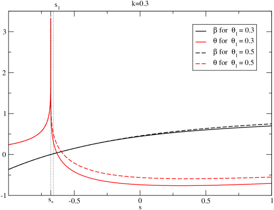
Figure 4: Solutions $\beta(s)=\alpha(s)^{-1}$ and $\theta(s)$ in the case of Christodoulou’s system (6.1)–(6.2). The matching of the solution at $s=s_{*}$ is shown for two different values of the parameter $\theta_{1}=\theta(s_{1})$.

In Figure 4 are shown the numerical solutions of the differential system (6.1–(6.2), for $K_{0}=0.3$ and with two different values of $\theta_{1}=\theta(s_{1})$. We have numerically observed that, if the parameter $\epsilon$ was small enough and for any value of $\theta_{1}$, the backward integration detailed here-above would always bring back to the solution $\beta(s_{*})=0$ and $\theta(s_{*})=1/k$. We were thus able to numerically recover the result by Christodoulou [7] that, for a given $k<1$, each solution of the system (6.1)–(6.2) connects to a one-parameter family of solutions at $s=s_{*}$.

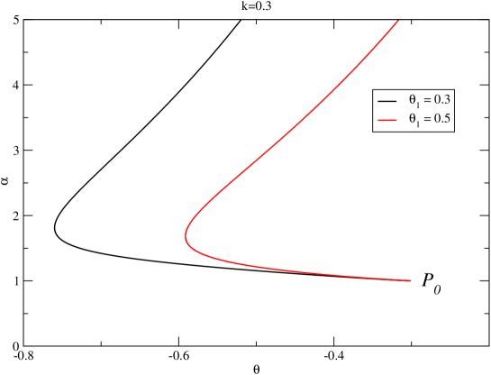
Figure 5: Trajectories in $(\theta,\alpha)$ plane of the two solutions shown in Figure 4. In both cases, the stationary point $\mathcal{P}_{0}:(1,-k)$ is reached as $s\to+\infty$.

By varying the parameter $\theta_{1}$, one can reach different asymptotic regimes, when $s\to+\infty$: both fields $\alpha$ and $\theta$ can diverge or they can converge to the stationary point $\mathcal{P}_{0}:(\alpha=1,\theta=-k)$. This last case is displayed in Figure 5, with the trajectories of the solutions in the $(\theta,\alpha)$ plane. (This is to be compared with Figure 4 in [7].)

6.3 Numerical solutions of the reduced system

In the case of interest in this paper, we have to deal with the matching of four fields $(\alpha,\Theta,\xi,K)$ at $s=s_{*}$. We use the same numerical technique, with the four steps described at the beginning of this section. We have numerically observed that here, in addition to $\theta_{1}$($\Theta_{1}=\Theta(s_{1})$), we need to specify the value of $\xi_{1}=\xi(s_{1})$. On the other hand, near an equilibrium point $U_{K_{*}}$, with $0<K_{*}<1$ we get from the first and last equations in (3.2):

$$\beta^{\prime}(s)\sim 1-K_{*}^{2},\qquad\quad K^{\prime}(s)\sim\sigma K_{*}\xi_{*},$$

so that we can write the following expansions:

$$\beta(s) ={}\left(1-K_{*}^{2}\right)\left(s-s_{*}\right)+o\left(\left|s-s_{*}\right|\right),$$ (6.7)

$$K(s) ={}K_{*}-\frac{\sigma^{2}K_{*}}{K_{*}^{2}+\sigma^{2}}\left(s-s_{*}\right)+o\left(\left|s-s_{*}\right|\right).$$ (6.8)

We can therefore obtain numerical estimations of the values of these two fields at $s=s_{1}$ and perform the integration backward, from $s_{1}$ toward $s_{*}$. We again do the shift in $s$ to match $\beta$ up to machine precision at $s=s_{*}$, but doing so does not allow for an accurate matching of $K(s)$. We then do several (usually no more than five) integrations from $s_{1}$ toward $s_{*}$, correcting each time the starting value $K(s_{1})$ in such a way that, at the end, the function $K(s)$ is continuous at $s_{*}$, up to machine precision.

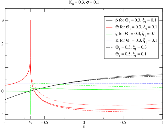
Figure 6: Solutions $\beta\left(=\alpha^{-1}\right),\Theta,\xi$ and $K$ of the reduced system (3.2). The matching of the fields at $s=s_{*}$ are shown for three sets of the parameters $\left(\Theta_{1}=\Theta(s_{1}),\xi_{1}=\xi(s_{1})\right)$.

Results are displayed in Figure 6, where we have taken $K_{0}=0.3$ and $\sigma=0.1$. The matching of all four fields are done with the setting of two new parameters $\left(\Theta_{1},\xi_{1}\right)$, which seems to indicate that a solution starting from the interior region ($s<s_{*}$) connects to a two-parameter family of solutions in the exterior region ($s>s_{*}$). Depending on these two parameters $\left(\Theta_{1},\xi_{1}\right)$, we numerically recover a behavior similar to that of Christodoulou’s system [7]: for some values of $k,\sigma,\Theta_{1}$ and $\xi_{1}$, the system can converge to the stationary point (b) of Section 4.2, that is, $\left(1,-K^{*},0,K^{*}\right)$ with

$$K^{*}=\lim_{s\to+\infty}K(s).$$ (6.9)

Figure 7: Trajectories of the solutions of the reduced system (3.2) in the $(\theta,\alpha,\xi)$ space, for three different sets of parameters $\left(\Theta_{1},\xi_{1}\right)$.

Part of this behavior is displayed in Figure 7, where the trajectories in the $\left(\theta,\alpha,\xi\right)$ space, for three sets of parameters $\left(\Theta_{1},\xi_{1}\right)$. Each set of parameters can lead a priori to a different limit $P_{K^{*}}$. If these trajectories were projected onto the $(\alpha,\Theta)$ plane, they would resemble a lot the ones of the general-relativistic system of Figure 5, studied by Christodoulou [7], with the noticeable difference that we no longer have a single limit $\mathcal{P}_{0}$, but the endpoint depends in general on the value $K^{*}$ (see (6.9)), which changes from one set of parameters to another.

7 Conclusions

We have studied the formation of naked singularities in the process of the gravitational collapse of a real massless scalar field, and have generalized Christodoulou’s construction of a family of spacetimes containing a naked singularity. While Christodoulou worked within the classical Einstein theory, we have here considered the Brans-Dicke theory. This effectively led us to deal with a new scalar field and to promote Christodoulou’s constant parameter $k$ to a dynamical variable $K$.

We were able to fully analyze the interior region and rigorously justify the matching across the past light-cone of the naked singularity. Partial analytical information was also obtained in the exterior region, and we finally completed our study with numerical simulations. We could show that the variable $K$ always decreases from any initial value to a value $K_{*}$ smaller than $1$ at the past light-cone. This eliminates the possibility in Christodoulou’s work of forming pathological solutions without a past light-cone. In that sense the addition of the Brans-Dicke field has a “regularizing” effect. The behavior of the solutions in the exterior region is similar to the one of Christodoulou’s solution and, in fact, the Brans-Dicke field vanishes on the future light-cone of the singularity (a Cauchy horizon). However, the dynamical structure of the phase space is quite different, as our phase space is much larger and does not contain Christodoulou’s case as a subspace.

Like Christodoulou established for solutions to the classical Einstein equations, our solutions are probably highly unstable against small (radially symmetric, for instance) perturbations.

It is quite reasonable to expect that more general scalar-tensor theories would exhibit a similar behavior. In particular, it would be interesting to extend our conclusions to the more general models arising in the so-called $f(R)$ theories of gravity when the action involves a nonlinear function of the Ricci scalar.

Acknowledgments

The authors were supported by the Agence Nationale de la Recherche (ANR) through the grant 06-2-134423 entitled “Mathematical Methods in General Relativity” (Math-GR). JMM was also supported by the French ANR grant BLAN07-1_201699 entitled “LISA Science”, and also in part by the Spanish MICINN projects FIS2009-11893 and FIS2008-06078-C03-03. PLF and JMM acknowledge support from the Erwin Schrödinger Institute, Vienna, during the program “Quantitative Studies of Nonlinear Wave Phenomena”, organized by P.C. Aichelburg, P. Bizoń, and W. Schlag.

References

References

• [1] Babichev, E., and Langlois, D., Relativistic stars in f(R) gravity, Phys. Rev. D. 80, p. 121501 (2009).
• [2] Bergmann, P.G., Comments on the scalar-tensor theory, Int. J. Theor. Phys. 1, p. 25 (1968).
• [3] Bondi, H., van der Burg, M.G.J. and Metzner, A.W.K., Gravitational waves in general relativity VII, Proc. R. Soc. London A269, p. 21 (1962).
• [4] Brady, P.R., Self-similar scalar field collapse: naked singularities and critical behavior, Phys. Rev. D 51, p. 4168 (1995).
• [5] Brady, P.R., Choptuik, M.W., Gundlach, C. and Neilsen, D.W., Black-hole threshold solutions in stiff fluid collapse, Class. Quantum Grav. 19, p. 6359 (2002).
• [6] Brans, C., and Dicke, R.H., Mach’s principle and a relativistic theory of gravitation, Phys. Rev. 124, p. 925 (1961).
• [7] Christodoulou, D., Examples of naked singularity formation in the gravitational collapse of a scalar field, Ann. of Math. 140, p. 607 (1994).
• [8] Christodoulou, D., The instability of naked singularities in the gravitational collapse of a scalar field, Ann. Math. 149, p. 183 (1999).
• [9] Christodoulou, D., On the global initial value problem and the issue of singularities, Class. Quantum Grav. 16, p. A23 (1999).
• [10] Choptuik, M., Universality and scaling in gravitational collapse of a massless scalar field, Phys. Rev. Lett. 70, p. 9 (1993).
• [11] Damour, T., and Esposito-Farèse, G., Tensor-multi-scalar theories of gravitation, Class. Quantum Grav. 9, p. 2093 (1992)
• [12] Fierz, M., On the physical interpretation of Jordan’s extended theory of gravitation, Helv. Phys. Acta 29, p. 128 (1956)
• [13] Gundlach, C., The Choptuik spacetime as an eigenvalue problem, Phys. Rev. Lett. 75, p. 3214 (1995).
• [14] Martín-García, J.M., and Gundlach, C., Global structure of Choptuik’s critical solution in scalar field collapse, Phys. Rev. D 68, p. 024011 (2003).
• [15] Gundlach, C., and Martín-García, J.M., Kinematics of discretely self-similar spherically symmetric spacetimes, Phys. Rev. D 68, p. 064019 (2003).
• [16] Jordan, P., Zum gegenwärtigen stand der Diracschen kosmologischen hypothesen, Z. Phys. 157, p. 112 (1959)
• [17] Hirschmann, E.W., and Eardley, D.M., Universal scaling and echoing in the gravitational collapse of a compplex scalar field, Phys. Rev. D 51 p. 4198 (1995).
• [18] Hirschmann, E.W. and Eardley, D.M., Criticality and bifurcation in the gravitational collapse of a self-coupled scalar field, Phys. Rev. D 56, p. 4696 (1997).
• [19] Lake, K., and Zannias, T., Structure of singularities in the spherical gravitational collapse of a charged null fluid, Phys. Rev. D 43, p. 1798 (1991).
• [20] Lake, K., Naked singularities in gravitational collapse which is not self-similar, Phys. Rev. D 43, p. 1416 (1991).
• [21] Liebling, S.L., and Choptuik, M.W., Black hole criticality in the Brans-Dicke model, Phys. Rev. Lett. 77 p. 1424 (1996).
• [22] Gundlach, C., and Martín-García, J.M., Critical phenomena in gravitational collapse, Living Rev. Relativity 10 (2007), 5. See http://www.livingreviews.org/lrr-2007-5.
• [23] Nordtvedt, K., Post-newtonian metric for a general class of scalar-tensor gravitational theories and observational consequences, Astrophys. J. 161, p. 1059 (1970).
• [24] Pürrer, M. Global versus local aspects of critical collapse, Ph.D. Thesis, University of Vienna, 2007, ArXiv:gr-qc/0708.1914.
• [25] Santiago, D.I., Kalligas, D., and Wagoner, R.V., Nucleosynthesis constraints on scalar-tensor theories of gravity, Phys. Rev. D 56, p. 7627 (1997).
• [26] Siebel, F., Font, J.A., and Papadopoulos, P., Scalar field induced oscillations of relativistic stars and gravitational collapse , Phys. Rev. D 65, p. 024021 (2001).
• [27] Wagoner, R.V., Scalar-tensor theory and gravitational waves, Phys. Rev. D 1, p. 3209 (1970).
• [28] Wald, R.M., Gravitational collapse and cosmic censorship, Preprint, 1997, ArXiv:gr-qc/9710068 (unpublished).