Ground-state configuration space heterogeneity of random finite-connectivity spin glasses and random constraint satisfaction problems

Abstract

We demonstrate through two case studies, one on the $p$-spin interaction model and the other on the random $K$-satisfiability problem, that a heterogeneity transition occurs to the ground-state configuration space of a random finite-connectivity spin glass system at certain critical value of the constraint density. At the transition point, exponentially many configuration communities emerge from the ground-state configuration space, making the entropy density $s(q)$ of configuration-pairs a non-concave function of configuration-pair overlap $q$. Each configuration community is a collection of relatively similar configurations and it forms a stable thermodynamic phase in the presence of a suitable external field. We calculate $s(q)$ by the replica-symmetric and the first-step replica-symmetry-broken cavity methods, and show by simulations that the configuration space heterogeneity leads to dynamical heterogeneity of particle diffusion processes because of the entropic trapping effect of configuration communities. This work clarifies the fine structure of the ground-state configuration space of random spin glass models, it also sheds light on the glassy behavior of hard-sphere colloidal systems at relatively high particle volume fraction.

1 Introduction

Spin glass models defined on finite-connectivity random graphs have two control parameters, one is the temperature $T$ and the other is the interaction (or constraint) density, defined as the number $M$ of interactions (constraints) versus the number $N$ of vertices, $\alpha\equiv M/N$. Theoretical work of the last ten years [1, 2, 3] have established the understanding that, a random spin glass system with many-body interactions will experience a clustering transition if either the temperature $T$ is lowered below certain threshold value or the constraint density $\alpha$ is increased beyond certain threshold value. At the clustering transition, the configuration space of the system splits into an exponential number of Gibbs pure states and ergodicity is broken. This transition is followed by another phase transition of the configuration space, the condensation transition, as $T$ is further lowered or $\alpha$ further increased. At the condensation transition, a sub-exponential number of large Gibbs states start to dominate the configuration space and hence the equilibrium property of the system [3]. These properties were first observed in fully-connected mean-field spin glass models [4]. Whether they are also valid in $D$-dimensional real-world spin glass systems ($D=3$ or $D=2$) is still a debated open issue.

Although the configuration space geometric properties of random finite-connectivity spin glass models at or after the clustering transition have been well characterized by statistical physics methods, much less is known about the configuration space structure just before the clustering transition. Why do an exponential number of Gibbs states suddenly appear at the clustering transition? Are they preceded by precursor structures in the ergodic phase of the configuration space? If yes, when do the Gibbs-state precursors start to form and how to describe their evolution? What are the impacts of these precursor structures to the equilibrium dynamical properties of the system? These questions are important for a full understanding of the structural evolution of the configuration space.

In this paper, as a continuation of our recent efforts [5, 6, 7, 8], we study the fine structure of the configuration space of random finite-connectivity spin glass models in the vicinity of the clustering transition. We focus on the evolution of the ground-state configuration space (corresponding to $T=0$) using the constraint density $\alpha$ as the control parameter. As demonstrated through two case studies, a heterogeneity transition occurs to the ground-state configuration space at certain critical value of $\alpha$. At the transition point, exponentially many communities of configurations emerge from the ground-state configuration space. Each configuration community is a collection of relatively similar configurations and it forms a stable thermodynamic phase in the presence of a suitable external field; they are the precursors for the Gibbs states at the clustering transition. The entropy density $s(q)$ of configuration-pairs as a function of configuration-pair overlap $q$ is calculated by the replica-symmetric (RS) and the first-step replica-symmetry-broken (1RSB) cavity methods. Extensive numerical simulations are performed to confirm that, the entropic trapping effect of ground-state configuration communities leads to strong dynamical heterogeneity of diffusion processes within the configuration space.

Dynamical heterogeneity in the fully-connected $p$-spin interaction spherical model (with continuous spins) [9] was quantitatively investigated by Donati and co-workers [10] within the framework of the Franz-Parisi effective potential theory [11, 12]. The results of the present paper for finite-connectivity systems with discrete spins are qualitatively similar to the results of [10]. Some aspects of the heterogeneity transition in random finite-connectivity systems are also shared by real-world $D$-dimensional spin glass and structural glass systems, such as hard-sphere poly-disperse colloidal systems, where the particle volume fraction plays the role of the constraint density $\alpha$ [10]. In real-world glass systems and supercooled liquid systems, dynamic heterogeneity occurs in real space. The present work is also related to the work of Krzakala and Zdeborova on the adiabatic evolution of a single Gibbs state of a finite-connectivity spin glass system as a function of temperature $T$ [13, 14].

Two model systems are studied in the paper. Section 2 concerns with the $p$-body spin glass system, which is equivalent to the random $K$-XORSAT (exclusive-or-satisfiability) problem of computer science. Replica-symmetric and 1RSB mean-field calculations are carried out to obtain the entropy density of ground-state configuration-pairs. Section 3 focuses on the heterogeneity transition and the dynamical heterogeneity of the random $K$-satisfiability ($K$-SAT) problem. Results obtained by RS calculations and numerical simulations are reported in this section. We make further discussions in section 4.

2 The random $p$-body spin glass model

The random $p$-body spin glass model is defined by the energy function

$$E_{pspin}(\vec{\sigma})=-\sum\limits_{a=1}^{M}J_{a}\prod\limits_{i\in\partial a}\sigma_{i}\ ,$$ (1)

where $\vec{\sigma}\equiv(\sigma_{1},\sigma_{2},\ldots,\sigma_{N})$ denotes a spin configuration for the $N$ vertices $i\in[1,N]$, with each spin variable $\sigma_{i}\in\{-1,+1\}$; the index $a\in[1,M]$ denotes one of the $M$ interactions of the system and $J_{a}$ is the quenched random coupling constant, whose value is fixed to $J_{a}=+1$ or $J_{a}=-1$ with equal probability; the set $\partial a$ includes all the vertices that participate in the interaction $a$, its size is fixed to $p$, and each of its $p$ different elements is randomly and uniformly chosen from the whole set of $N$ vertices. Similar to $\partial a$, we denote by $\partial i$ the set of interactions that involve vertex $i$. While each interaction $a$ in the $p$-body spin glass model affects the same number $p$ of vertices, the sets $\partial i$ may have different sizes for different vertices $i$. Actually, when $N$ is large enough, the probability that a randomly chosen vertex participates in $k$ interactions is governed by the Poisson distribution $P_{P}(k)=e^{-c}c^{k}/k!$, with mean value $c=pM/N$.

In the $p$-body spin glass model (1), each interaction contributes either a positive energy $+1$ or a negative energy $-1$ to the total energy. If we set $p=K$, this model is equivalent to the random $K$-XORSAT problem with the energy function

$$E_{xorsat}(\vec{\sigma})=\sum\limits_{a=1}^{M}\frac{1-J_{a}\prod_{i\in\partial a}\sigma_{i}}{2}\ .$$ (2)

For the random $K$-XORSAT problem, each interaction $a$ is also referred to as a constraint, whose energy $(1-J_{a}\prod_{i\in\partial a}\sigma_{i})/2$ is either zero (constraint being satisfied) or unity (constraint violated). The energy $E_{xorsat}(\vec{\sigma})$ counts the total number of violated constraints by the spin configuration $\vec{\sigma}$. The constraint density $\alpha$ of the system is by $\alpha=M/N$.

The random $K$-XORSAT problem (or equivalently, the random $p$-body spin glass model) has been well studied in the statistical physics community. It serves as an interesting system for understanding the low-temperature equilibrium property of finite-connectivity spin glasses [1, 15, 16, 17], and for understanding the dynamical property of glassy systems [18, 19]. This model is also closely related to error-correcting code systems of information science, such as the Sourlas code [20]. The ground-state configuration space structure of the random $K$-XORSAT problem has been investigated in great detail [16, 17, 21] and was found to depend only on $K$ and the constraint density $\alpha$ in the limit of $N\rightarrow\infty$.

For a given value of $K\geq 2$ there is a satisfiability threshold $\alpha_{s}(K)$. When the constraint density $\alpha$ is below $\alpha_{s}(K)$, the ground-state energy of model (2) is zero (the system is in the SAT phase), but it becomes positive when $\alpha>\alpha_{s}(K)$ (the UNSAT phase). A zero-energy spin configuration of model (2) is referred to as a solution, and all the solutions form the solution space $\mathcal{S}$ of this system. The solution space of a large random $K$-XORSAT problem is non-empty only if its constraint density is in the range of $\alpha\leq\alpha_{s}(K)$. We have $\alpha_{s}(2)=0.5$, $\alpha_{s}(3)=0.918$, and $\alpha(4)=0.977$ [16].

Before the solution space of the random $K$-XORSAT ($K\geq 3$) becomes empty at $\alpha>\alpha_{s}(K)$, it experiences an ergodicity-breaking (clustering) transition at the threshold value $\alpha=\alpha_{d}(K)$, with $\alpha_{d}(3)=0.818$ and $\alpha_{d}(4)=0.772$ [16]. For $\alpha<\alpha_{d}(K)$, the whole solution space forms a single Gibbs state (the meaning of a Gibbs state is explained geometrically in the following subsection). On the other hand, for $\alpha>\alpha_{d}(K)$, the solution space is no longer ergodic but is composed of exponentially many solution clusters (Gibbs states), each of which containing exactly the same number of solutions. For $\alpha_{d}(K)<\alpha<\alpha_{s}(K)$, solutions from different solution clusters are separated by energy barriers that are proportional to the vertex number $N$ [18].

2.1 Non-concavity of the entropy function and solution space heterogeneity

The similarity of two solutions $\vec{\sigma}^{1}$, $\vec{\sigma}^{2}$ in the non-empty solution space $\mathcal{S}$ of a random $K$-XORSAT problem can be measured by the overlap value

$$q(\vec{\sigma}^{1},\vec{\sigma}^{2})=\frac{1}{N}\sum\limits_{i=1}^{N}\sigma_{i}^{1}\sigma_{i}^{2}\ .$$ (3)

We denote by $\mathcal{N}(q)$ the total number of solution-pairs in the solution space $\mathcal{S}$ with an overlap value $q$. This number is exponential in $N$ in the SAT phase $\alpha\leq\alpha_{s}(K)$. Therefore in the limit of large $N$, an entropy density $s(q)$ is defined as

$$s(q)=\frac{1}{N}\ln\mathcal{N}(q)\ .$$ (4)

The entropy density function $s(q)$ contains rich information about the structure of the solution space $\mathcal{S}$ (see figure 1). The shape of $s(q)$ has several qualitative changes as the constraint density $\alpha$ increases. The first qualitative change occurs at $\alpha=\alpha_{cm}$, where $s(q)$ becomes non-concave. This concavity change corresponds to the formation of (exponentially) many solution communities in the solution space (the large-scale homogeneity of the solution space is then broken) [6, 7]. We refer to $\alpha_{cm}$ as the heterogeneity transition point.

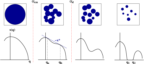
Figure 1: Non-concavity of the entropy function $s(q)$ as defined by (4) and the large scale organization of the solution space of a random constraint satisfaction problem. $s(q)$ is a concave function of the solution-pair overlap $q$ when the constraint density $\alpha$ is low enough (left-most panel); at $\alpha=\alpha_{cm}$, $s(q)$ starts to be non-concave, marking the formation of many solution communities in the solution space (second panel from left); then as $\alpha$ increases to $\alpha=\alpha_{d}$, $s(q)$ becomes non-monotonic, the solution communities separate into different solution clusters and ergodicity of the solution space is broken; the solution clusters shrink in size as $\alpha$ further increases, and eventually the number of solution-pairs with intermediate overlap values $q\in[q_{1},q_{2}]$ will be zero and $s(q)$ is only positive for $q>q_{2}$ and $q<q_{1}$.

We introduce the following partition function $Z(x)$ for the solution space $\mathcal{S}$ [7]

$$Z(x)=\sum\limits_{\vec{\sigma}^{1}\in\mathcal{S}}\sum\limits_{\vec{\sigma}^{2}\in\mathcal{S}}\exp\Bigl{(}x\sum\limits_{i=1}^{N}\sigma_{i}^{1}\sigma_{i}^{2}\Bigr{)}=\sum\limits_{q}\exp\Bigl{[}N\bigl{(}s(q)+xq\bigr{)}\Bigr{]}\ ,$$ (5)

where $x$ is a coupling field between the solutions. When $x$ is positive, solution-pairs with larger overlap values have larger weights in the partition sum (5). Under the field $x$, the mean solution-pair overlap value is $\overline{q}(x)=(1/N){\rm d}\ln Z(x)/{\rm d}x$. For $N\rightarrow\infty$, we see from (5) that, $\overline{q}(x)=\arg\,\max_{q}\bigl{(}s(q)+xq\bigr{)}$. At $x=0$, $\overline{q}(0)$ is equal to $q_{0}$, the most probable solution-pair overlap value of the solution space.

If the entropy density $s(q)$ is concave in $q\in[q_{0},1]$, then $\overline{q}(x)$ increases continuously with $x$ for $x\geq 0$. However if $s(q)$ is non-concave, because there exists a line of slope $-x^{*}$ which touches $s(q)$ at two different points $q=q_{a}$ and $q=q_{b}>q_{a}$ (figure 1), then the value of $\overline{q}(x)$ jumps from $q_{a}$ to $q_{b}$ at $x=x^{*}$ [6, 7]. This discontinuity of $\overline{q}(x)$ reveals the existence of a field-induced first-order phase transition at $x=x^{*}$. The solution-pairs exhibit two different levels of similarity. For $x>x^{*}$, the partition function $Z(x)$ are contributed overwhelmingly by (intra-community) solution-pairs with overlap values $\geq q_{b}$ (overlap-favored phase), while for $x<x^{*}$, $Z(x)$ is dominated by (inter-community) solution-pairs with overlap values $\leq q_{a}$ (entropy-favored phase). The difference $q_{b}-q_{a}$ increases from zero as the constraint density $\alpha$ exceeds the critical value $\alpha_{cm}$. At $\alpha=\alpha_{cm}$, the solution space is in a critical state, where the boundaries between different solution communities are elusive, and the field-induced phase transition is second-order.

The Hamming distance between two solutions $\vec{\sigma}^{1}$ and $\vec{\sigma}^{2}$ is defined as $D(\vec{\sigma}^{1},\vec{\sigma}^{2})\equiv\sum_{i=1}^{N}(1-\sigma_{i}^{1}\sigma_{i}^{2})/2$, which is related to the solution-pair overlap by $D(\vec{\sigma}^{1},\vec{\sigma}^{2})=(N/2)(1-q(\vec{\sigma}^{1},\vec{\sigma}^{2}))$. The solution space $\mathcal{S}$ can be represented by a graph of nodes and edges. Each node of this solution graph denotes a solution, and an edge is linked between two nodes of the graph if the corresponding two solutions has a Hamming distance not exceeding a specified value $D_{0}$. For the random $K$-XORSAT problem at $\alpha<\alpha_{d}(K)$, there exists a minimum value of $D_{0}\ll N$ such that all the nodes of the solution graph are in a single connected component [18]. We take this minimum value as our edge linking criterion. (For $\alpha>\alpha_{d}(K)$, if $D_{0}$ is not of the same order as $N$, the solution graph will be a collection of exponentially many disjointed components.) In the ergodic phase of $\alpha<\alpha_{d}(K)$, we may introduce two particles to the solution graph. Initially these two particles are residing on the same node, say $\vec{\sigma}^{0}$, of the graph. In case the particles are uncoupled, then each particle performs a random diffusion in the solution graph independent of the other: Suppose at time $t$ the particle is at node $\vec{\sigma}$, then at the next time step it will, with probability $k_{\vec{\sigma}}/k_{max}$, make a move to a randomly chosen nearest-neighbor of this node, where $k_{\vec{\sigma}}$ is the number of attached edges (the degree) of node $\vec{\sigma}$, and $k_{max}$ is the maximal node degree in the solution graph. In the case the particles are coupled by a field $x$, however, the particle diffusions are mutually influenced, and the visited node-pairs (say $\vec{\sigma}^{1}$ and $\vec{\sigma}^{2}$) are no longer uniformly distributed but are favored to more similar pairs by a factor of $e^{xNq(\vec{\sigma}^{1},\vec{\sigma}^{2})}$. In the thermodynamic limit $N\rightarrow\infty$, when the coupling field $x$ is larger than $x^{*}$, then even at time approaching infinity, the two particles will still be diffusing in the neighborhood of each other and in the neighborhood of the initial node $\vec{\sigma}^{0}$. Such a strong memory effect at field value $x>x^{*}$ is a dynamical manifest of the existence of communities in the solution space.

2.2 Annealed approximation for $s(q)$

If one knows a solution $\vec{\sigma}^{1}=(\sigma_{1}^{1},\sigma_{2}^{1},\ldots,\sigma_{N}^{1})$ for the $K$-XORSAT system (2), it is convenient to perform a gauge transform ${\sigma}_{i}\leftarrow\sigma_{i}\sigma_{i}^{1}$ to the spin value of each vertex $i$. Under this transform, (2) is simplified to

$$E(\vec{\sigma})=\sum\limits_{a=1}^{M}\frac{1-\prod_{i\in\partial a}\sigma_{i}}{2}\ .$$ (6)

In this transformed system, all the coupling constants are positive ($J_{a}=+1$), and the overlap of the transformed solution $\vec{\sigma}$ with the reference solution $\vec{\sigma}^{1}$ is $q(\vec{\sigma})=(1/N)\sum_{i}\sigma_{i}$. Equation (6) is independent of the reference solution $\vec{\sigma}^{1}$. This is a well-known property of the $K$-XORSAT problem, namely its solution space $\mathcal{S}$ has the same local and global structure when viewed from any of its solutions. Because of this nice property, instead of calculating the solution-pair number $\mathcal{N}(q)$, we calculate the number $\mathcal{N}_{1}(q)$ of solutions which have an overlap value $q$ with a reference solution $\vec{\sigma}^{1}$. We denote the corresponding entropy density also as $s(q)$, i.e., $s(q)=(1/N)\ln\mathcal{N}_{1}(q)$. (With this slight abuse of notation, the solution-pair entropy density as defined by (4) is $s(q)+s_{0}(\alpha)$, where $s_{0}(\alpha)$ is the entropy density of the whole solution space at constraint density $\alpha$.)

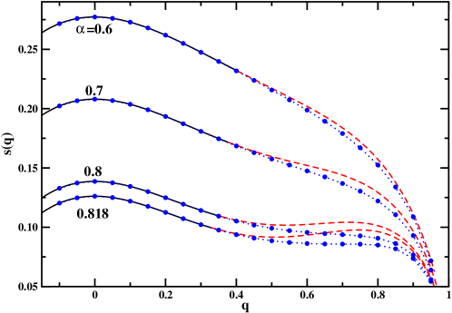
Figure 2: The entropy density $s(q)$ of solutions at an overlap level $q$ to a reference solution for the random $K$-XORSAT problem with $K=3$ and $\alpha=0.6$, $0.7$, $0.8$, $0.818$ (from top to bottom). Black solid lines and red dashed lines are results obtained by the annealed approximation (8), and blue dots are results of the replica-symmetric cavity method (dotted lines just for guiding the eye). When (12) is valid, expression (8) gives the exact mean value of $s(q)$, but if it is violated, (8) is only an upper-bound for the mean value of $s(q)$.

The average value of $\mathcal{N}_{1}(q)$ over the ensemble of random $K$-XORSAT problems with fixed vertex number $N$ and constraint density $\alpha$ is

$$\overline{\mathcal{N}_{1}(q)}=\left(\begin{array}[]{c}N\\ (q+1)N/2\end{array}\right)\left(\frac{1+q^{K}}{2}\right)^{\alpha N}$$ (7)

For $N\rightarrow\infty$ we obtain the following annealed approximation for $s(q)$ as

$$s_{ann}(q)\equiv\frac{\ln\overline{\mathcal{N}_{1}(q)}}{N}=-\frac{1+q}{2}\ln\frac{1+q}{2}-\frac{1-q}{2}\ln\frac{1-q}{2}+\alpha\ln\frac{1+q^{K}}{2}\ .$$ (8)

For $K=3$, the function $s_{ann}(q)$ is concave in $q$ only for $\alpha<0.577$. For $0.577<\alpha<0.778$, $s_{ann}(q)$ is non-concave in $q$ but is still monotonic in the range $q\in[0,1]$; the monotonicity of $s_{ann}(q)$ in $q\in[0,1]$ is lost when $\alpha$ exceeds $0.778$ (figure 2). The same qualitative results are obtained for the random $K$-XORSAT problem with $K\geq 4$.

The annealed approximation $s_{ann}(q)$ is an upper bound of the entropy density $s(q)$ for a typical random $K$-XORSAT problem. These two quantities are identical only when $\mathcal{N}_{1}(q)$ has the self-averaging property, i.e., the value distribution of $\mathcal{N}_{1}(q)$ among the ensemble of random $K$-XORSAT problems of constraint density $\alpha$ approaches a delta function in the limit of $N\rightarrow\infty$. To check whether this self-averaging property is valid, we need to calculate the mean value of $\mathcal{N}_{1}^{2}(q)$. After some combinatorial analysis, we obtain

$$\overline{\mathcal{N}_{1}^{2}(N)}=\left(\begin{array}[]{c}N\\ (1+q)N/2\end{array}\right)\sum\limits_{n}\left(\begin{array}[]{c}(1+q)N/2\\ n\end{array}\right)\left(\begin{array}[]{c}(1-q)N/2\\ n\end{array}\right)Q_{n}^{\alpha N}\ ,$$ (9)

where $Q_{n}=[1+2q^{K}+(1-4n/N)^{K}]/4$. In the $N\rightarrow\infty$ limit, we therefore have

$$\frac{1}{N}\ln\overline{\mathcal{N}_{1}^{2}(q)}=\max\limits_{0\leq\rho\leq\min\left(\frac{1-q}{2},\frac{1+q}{2}\right)}s_{2}(q,\rho)\ ,$$ (10)

with $s_{2}(q,\rho)$ being expressed as

$$s_{2}(q,\rho)= -\frac{1+q}{2}\ln\frac{1+q}{2}-\frac{1-q}{2}\ln\frac{1-q}{2}-\rho\ln\frac{4\rho^{2}}{1-q^{2}}$$ (11)

$$-\left(\frac{1-q}{2}-\rho\right)\ln\left(1-\frac{2\rho}{1-q}\right)-\left(\frac{1+q}{2}-\rho\right)\ln\left(1-\frac{2\rho}{1+q}\right)$$

$$+\alpha\ln\frac{1+2q^{K}+(1-4\rho)^{K}}{4}\ .$$

Self-averaging of $\mathcal{N}_{1}(q)$ requires that

$$\Delta\equiv\max\limits_{0\leq\rho\leq\min\left(\frac{1-q}{2},\frac{1+q}{2}\right)}s_{2}(q,\rho)-s_{ann}^{2}(q)=0\ .$$ (12)

Numerical calculations reveal that (12) is satisfied only for values of $q$ very close to $0$ or very close to $1$. In figure 2, $s_{ann}(q)$ is plotted as a black solid line if $\Delta<10^{-3}$ and as a red dashed line if $\Delta\geq 10^{-3}$.

As $s_{ann}(q)$ is only an upper bound to $s(q)$, the fact that $s_{ann}(q)$ becomes non-concave at $\alpha<\alpha_{d}(K)$ can not be used as a proof that $s(q)$ also becomes non-concave at $\alpha<\alpha_{d}(K)$. We proceed to calculate $s(q)$ by the cavity method of statistical physics.

2.3 Replica-symmetric mean-field analysis

For the gauge-transformed $K$-XORSAT system (6), if vertex $i$ is involved in constraint $a$, we define a cavity probability $p_{i\rightarrow a}^{+}$ as the probability that $\sigma_{i}$ takes the value $\sigma_{i}=+1$ when the constraint $a$ is absent. For each constraint $a$ we exploit the Bethe-Peierls approximation [1, 22, 23] and assume that, the spin states of the vertices $j\in\partial a$ are mutually independent in the absence of $a$. Under this approximation, we obtain that if the vertex $i\in\partial a$ takes the spin value $\sigma_{i}$, the probability that constraint $a$ being satisfied is equal to $[1+\sigma_{i}\prod_{j\in\partial a\backslash i}(2p_{j\rightarrow a}^{+}-1)]/2$, where $\partial a\backslash i$ means the subset of $\partial a$ that is missing element $i$. Then the following belief-propagation equation can be written down for each vertex-constraint association $(i,a)$:

$$p_{i\rightarrow a}^{+}=\hat{p}(\{p_{j\rightarrow b}^{+}\})=\frac{e^{x}\prod\limits_{b\in\partial i\backslash a}\left[\frac{1+\prod\limits_{j\in\partial b\backslash i}(2p_{j\rightarrow b}^{+}-1)}{2}\right]}{e^{x}\prod\limits_{b\in\partial i\backslash a}\left[\frac{1+\prod\limits_{j\in\partial b\backslash i}(2p_{j\rightarrow b}^{+}-1)}{2}\right]+e^{-x}\prod\limits_{b\in\partial i\backslash a}\left[\frac{1-\prod\limits_{j\in\partial b\backslash i}(2p_{j\rightarrow b}^{+}-1)}{2}\right]}\ .$$ (13)

For a given energy function (6), there are $M\times K$ iteration equations, which form the replica-symmetric cavity theory [1, 22, 23].

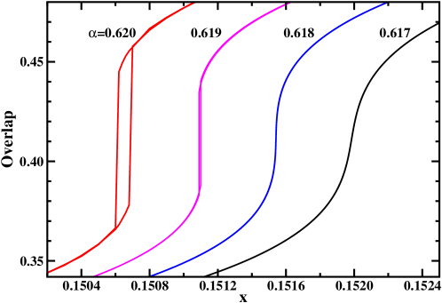
Figure 3: The mean overlap $\overline{q}(x)$ for the random $3$-XORSAT problem at $\alpha=0.617$, $0.618$, $0.619$, $0.620$ (from right to left). For $\alpha<\alpha_{cm}(K=3)=0.618154$, $\overline{q}(x)$ is a continuous function of $x$. At $\alpha=\alpha_{cm}(3)$, the slope of $\overline{q}(x)$ diverges at $x=0.151473$. For $\alpha>\alpha_{cm}(3)$, $\overline{q}(x)$ is discontinuous and has a hysteresis loop.

After this set of belief-propagation iteration equations has reached a fixed point, the mean overlap with the reference solution is calculated as

$$\overline{q}(x)=\frac{1}{N}\sum\limits_{i=1}^{N}\frac{e^{x}\prod\limits_{a\in\partial i}\left[\frac{1+\prod\limits_{j\in\partial a\backslash i}(2p_{j\rightarrow a}^{+}-1)}{2}\right]-e^{-x}\prod\limits_{a\in\partial i}\left[\frac{1-\prod\limits_{j\in\partial a\backslash i}(2p_{j\rightarrow a}^{+}-1)}{2}\right]}{e^{x}\prod\limits_{a\in\partial i}\left[\frac{1+\prod\limits_{j\in\partial a\backslash i}(2p_{j\rightarrow a}^{+}-1)}{2}\right]+e^{-x}\prod\limits_{a\in\partial i}\left[\frac{1-\prod\limits_{j\in\partial a\backslash i}(2p_{j\rightarrow a}^{+}-1)}{2}\right]}\ .$$ (14)

And the entropy density as a function of $x$ is

$$s(x)=\frac{1}{N}\sum\limits_{i=1}^{N}\ln\left(e^{x}\prod\limits_{a\in\partial i}\left[\frac{1+\prod\limits_{j\in\partial a\backslash i}(2p_{j\rightarrow a}^{+}-1)}{2}\right]+e^{-x}\prod\limits_{a\in\partial i}\left[\frac{1-\prod\limits_{j\in\partial a\backslash i}(2p_{j\rightarrow a}^{+}-1)}{2}\right]\right)$$

$$-\frac{1}{M}\sum\limits_{a=1}^{M}(K-1)\ln\left(\frac{1+\prod\limits_{j\in\partial a}(2p_{j\rightarrow a}^{+}-1)}{2}\right)-x\overline{q}(x)\ .$$ (15)

The mean value of $s(x)$ as averaged over the ensemble of random $K$-XORSAT problems (at fixed value of $\alpha$) can be calculated using the population dynamics technique [1, 21]. By eliminating $x$ from $s(x)$ and $\overline{q}(x)$ we obtain the entropy density function $s(q)$. The numerical results are shown in figure 2 (blue dots) for $K=3$ at different values of $\alpha$. The mean overlap function $\overline{q}(x)$ is shown in figure 3 for $K=3$ and $\alpha\approx 0.62$. Similar results are obtained for the cases of $K\geq 4$.

For the random $3$-XORSAT problem, $\overline{q}(x)$ is a continuous and smooth function of field $x$ when $\alpha<\alpha_{cm}(3)\simeq 0.6182$. As $\alpha$ approaches $\alpha_{cm}$ from below, however, the maximal slope of $\overline{q}(x)$ is proportional to $(\alpha_{cm}(3)-\alpha)^{-1}$ and diverges at $\alpha_{cm}(3)$. This divergence is a consequence of the fact that the entropy density $s(q)$ starts to be non-concave at $\alpha=\alpha_{cm}(3)$. For $\alpha>\alpha_{cm}(3)$, $\overline{q}(x)$ as calculated by the RS cavity theory shows discontinuity and hysteresis behavior when $x$ is close to certain threshold value $x^{*}$, indicating the existence of two distinct phases of the solution space as viewed from the reference solution ($\vec{\sigma}^{1}$). One of the phases contains solution $\vec{\sigma}^{1}$ and the other similar solutions, whose overlap with $\vec{\sigma}^{1}$ is larger than certain characteristic value $\approx(q_{a}+q_{b})/2$, see figure 1. We regard this phase as the solution community of solution $\vec{\sigma}^{1}$. If we choose another solution outside the solution community of $\vec{\sigma}^{1}$, we will find that this new reference solution is also associated with a different solution community.

For $\alpha_{cm}(K)<\alpha<\alpha_{d}(K)$, the solution space of the random $K$-XORSAT problem is therefore formed by exponentially many solution communities. As the solution space is very heterogeneous at this range of $\alpha$, the replica-symmetric mean-field theory probably is not sufficient to describe its statistical property. We now proceed to study the solution space heterogeneity using the 1RSB cavity theory.

2.4 First-step replica-symmetry-broken mean-field analysis

For the gauge-transformed model (6) under the coupling field $x$, to apply the 1RSB mean-field theory, the solution space is first divided into an exponential number of Gibbs states $\gamma$ [1, 21]. Each Gibbs state $\gamma$ represents a subspace $\mathcal{S}_{\gamma}\subset\mathcal{S}$, and its partition function is defined as

$$Z_{\gamma}(x)=\sum\limits_{\vec{\sigma}\in\mathcal{S}_{\gamma}}\exp\left(x\sum_{i=1}^{N}\sigma_{i}\right)\ .$$ (16)

We can then define a $`$free energy’ density $f_{\gamma}(x)$ as $f_{\gamma}=(1/N)\ln Z_{\gamma}(x)$. This free energy density is the sum of two parts, $f_{\gamma}=s_{\gamma}+xq_{\gamma}$, where $s_{\gamma}$ is the entropy density of Gibbs state $\gamma$ and $q_{\gamma}$ is the mean overlap level of solutions in $\mathcal{S}_{\gamma}$ to the reference solution $\vec{\sigma}^{1}$.

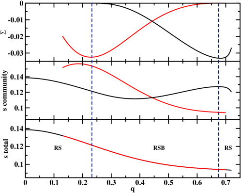
Figure 4: Results of the $m=1$ 1RSB mean-field theory for the random $3$-XORSAT problem with $\alpha=0.80$. The complexity, the entropy density of solution communities, and the total entropy density are shown in the upper, middle, and lower panel, respectively, as a function of the overlap $q$. Two sets of 1RSB mean-field results are obtained in the population dynamics when different types of initial values are used for the population. At each value of $q$, the result with the larger value of complexity and the smaller value of community entropy density should be considered. The two vertical dashed lines mark the boundary between the replica-symmetric (RS) and the replica-symmetry-broken (RSB) region.

The total 1RSB partition function of the system is

$$Z_{1RSB}\equiv\sum\limits_{\gamma}(Z_{\gamma})^{m}=\sum\limits_{\gamma}e^{Nmf_{\gamma}}=\int{\rm d}f\exp\left(N[\Sigma(f)+mf]\right)\ .$$ (17)

In the above equation, $m$ is the Parisi parameter, and $\Sigma(f)$ is the complexity, which measures the $`$entropy density’ of Gibbs states at the free energy density level $f$ [1, 21]. If we set $m=1$ in (17), each Gibbs state contributes a term $e^{Nf_{\gamma}}$ to $Z_{1RSB}$, and then $Z_{1RSB}$ is the total partition function of the system, provided that the complexity $\Sigma(f)$ calculated at $m=1$ is non-negative. The existence of a nontrivial 1RSB solution at $m=1$ is also a signature of the instability of the RS theory of the previous subsection [2, 3]. We therefore set $m=1$ in our calculations. The details of the 1RSB cavity mean field theory are presented in A, and here we discuss some of the numerical results obtained by population dynamics on the random $3$-XORSAT problem.

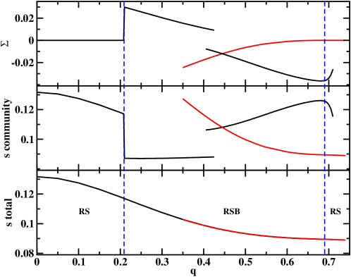
Figure 5: Same as figure 4, but for $\alpha=0.81$. The complexity $\Sigma(q)$ is positive for $0.21\leq q\leq 0.425$.

At $\alpha<\alpha_{cm}(3)$, no nontrivial 1RSB mean field results are obtained. The fixed point of the 1RSB population dynamics reduces to that of the RS theory for all the overlap values $0\leq q\leq 1$. As $\alpha$ exceeds $\alpha_{cm}(3)$, the replica-symmetric mean field theory becomes unstable for intermediate values of overlap $q$, and nontrivial fixed points of the 1RSB mean-field population dynamics are observed. For example, at $\alpha=0.80$ we find that the complexity $\Sigma(q)$ is exactly zero for overlap value $q\leq 0.233$ and $q\geq 0.675$, and $\Sigma(q)$ is negative for $0.233<q<0.675$ (see figure 4). The fact that $\Sigma(q)=0$ for $q\geq 0.675$ suggests that, the solutions with overlap levels $q\geq 0.675$ to $\vec{\sigma}^{1}$ are in a single solution community. In the corresponding solution subgraph of this solution community, any two solutions (nodes) with the same Hamming distance $D$ to $\vec{\sigma}^{1}$ are connected by at least one path that involves only other solutions with the same Hamming distance $D$ to $\vec{\sigma}^{1}$ (i.e., the subspace of solutions having the same overlap $q$ ($\geq 0.675$) with $\vec{\sigma}^{1}$ is ergodic within itself).

The second message we get, from the fact that $\Sigma(q)<0$ for $0.233<q<0.675$, is that the solution subgraph formed by all the solutions at the same overlap level $q$ [$\in(0.233,0.675)$] to $\vec{\sigma}^{1}$ is not ergodic within itself but is divided into greatly many disjointed connected sub-components, with a sub-exponential number of dominating ones. In this overlap range, the community entropy density and the total entropy density as obtained by the $m=1$ 1RSB mean-field theory can only be regarded as upper bounds for the true values. One needs to work with $m<1$ to obtain better estimates for the community entropy density and the total entropy density.

The third message we get from $\Sigma(q)=0$ for $q\leq 0.233$ is that, the solutions with overlap levels to $\vec{\sigma}^{1}$ less than $0.233$ form an ergodic subspace within itself. More precisely, all the solutions at each overlap level $q$ ($\leq 0.233$) to $\vec{\sigma}^{1}$ are ergodic within themselves. The solutions in such a subspace of fixed overlap $q$ come from different solution communities, but they are connected with each other in the solution graph even when only the edges inside the subgraph are remained.

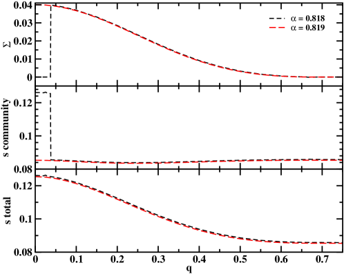
Figure 6: Same as figure 4, but for $\alpha=0.818$ and $\alpha=0.819$. At $\alpha=0.818$, the complexity $\Sigma(q)$ is positive for $0.038\leq q\leq 0.66$ and is negative ($\approx-10^{-5}$) for $0.66<q\leq 0.705$. At $\alpha=0.819>\alpha_{d}(3)$, the complexity $\Sigma(q)$ is positive even at $q=0$.

The theoretical results as shown in figure 5 and figure 6 for the random $3$-XORSAT problem at $\alpha=0.81$ and $\alpha=0.818$, respectively, are similar with the results of figure 4. At $\alpha=0.81$, the complexity $\Sigma(q)$ calculated at $m=1$ is positive for $0.21\leq q\leq 0.425$, indicating an exponential number of solution communities are equally contributing to the solution subspace at each overlap level $q\in[0.21,0.425]$. For an overlap level $q\in(0.425,0.69$], however, the solution subspace is again dominated by a sub-exponential number of large solution communities. The situation at $\alpha=0.818$ is similar, but the range of $q$ values for which $\Sigma(q)>0$ is further enlarged.

When the constraint density $\alpha$ exceeds the clustering transition point $\alpha_{d}(3)$, the complexity $\Sigma(q)$ at $m=1$ becomes positive at $q=0$ (see the exemplar case of $\alpha=0.819$ in figure 6). This result means that the largest subspace of solutions (with overlap level $q=0$ to $\vec{\sigma}^{1}$) becomes non-ergodic at $\alpha>\alpha_{d}(3)$, as expected.

2.5 Summary for $K$-XORSAT

The calculations of this section demonstrated that the solution space of the random $K$-XORSAT problem experiences a heterogeneity transition as the constraint density $\alpha$ approaches $\alpha_{cm}(K)$, where an exponential number of solution communities start to form in the solution space. These solution communities separate into different solution clusters at a larger constraint density value $\alpha_{d}(K)$, where an ergodicity-breaking transition occurs. For $\alpha_{cm}(K)<\alpha<\alpha_{d}(K)$, although the solution space as a whole is ergodic, the subspaces of solutions with intermediate overlap levels to a reference solution are non-ergodic within themselves.

Our theoretical results, combined with the results of [21] for $\alpha>\alpha_{d}(K)$, give a complete picture on the structural evolution of the solution space of the random $K$-XORSAT problem.

3 The random $K$-satisfiability problem

The random $K$-SAT problem is a famous model system for the study of typical-case computational complexity of NP-complete combinatorial satisfaction problems [24]. Its energy function $E(\vec{\sigma})$, like the random $K$-XORSAT problem, is defined as a sum over $M=\alpha N$ constraints $a$:

$$E(\vec{\sigma})=\sum\limits_{a=1}^{M}\prod\limits_{i\in\partial a}\frac{1-J_{a}^{i}\sigma_{i}}{2}\ .$$ (18)

In (18), each constraint $a$ affects a set $\partial a$ of $K$ randomly chosen vertices from the vertex set $\{1,2,3,\ldots,N\}$; $J_{a}^{i}$ is the preferred spin state of constraint $a$ on the vertex $i\in\partial a$, it takes the quenched value $+1$ or $-1$ with equal probability. If at least one of the vertices $i\in\partial a$ takes the spin value $\sigma_{i}=J_{a}^{i}$, the energy of the constraint $a$ is zero, otherwise its energy is unity. The solution space $\mathcal{S}$ of model (18) is formed by all the spin configurations $\vec{\sigma}$ of zero total energy (i.e., satisfying all the constraints). In model (18), each vertex $i$ is constrained by a set (denoted as $\partial i$) of constraints.

After the experimental demonstration of a satisfiability phase-transition in the random $3$-SAT problem by Kirkpatrick and Selman [24], studies on the solution space structure of the random $K$-SAT problem have been carried out through rigorous mathematical methods (see, e.g., [25, 26, 27]) and through statistical physics methods (see, e.g., [28, 29, 30, 3, 31, 32]). The threshold constraint density $\alpha_{s}(K)$ for the solution space to be empty is calculated to be $4.2667$ for the random $3$-SAT problem [30] and its values for $K\geq 4$ are also predicted by the 1RSB zero-temperature energetic cavity method [33]; a lower bound on $\alpha_{s}(K)$ is calculated by the zero-temperature long-range frustration theory [34, 8]. Ergodicity of the solution space is broken at the clustering transition point $\alpha=\alpha_{d}(K)<\alpha_{s}(K)$ [29, 30]. At $\alpha_{d}(K)\leq\alpha\leq\alpha_{s}(K)$, the solution space contains an exponential number of Gibbs states. The value of $\alpha_{d}(K)$ is calculated by the 1RSB zero-temperature entropic cavity method in [3, 35], reporting $\alpha_{d}(3)\simeq 3.87$ and $\alpha_{d}(4)\simeq 9.38$.

We are interested in the heterogeneity of the ergodic solution space at $\alpha<\alpha_{d}(K)$. In the following subsection we calculate the solution-pair mean overlap as defined by (3) using the replica-symmetric cavity method. The heterogeneity transition point $\alpha_{cm}(K)$ is determined by this RS mean-field theory.

3.1 Replica-symmetric mean-field analysis

The partition function (5) is a weighted sum over all the solution-pairs $(\vec{\sigma}^{1},\vec{\sigma}^{2})$. Each vertex is then associated with a spin vector-state $(\sigma_{i}^{1},\sigma_{i}^{2})$. Under the coupling field $x$, we define the cavity probability $\hat{p}_{a\rightarrow i}(\sigma,\sigma^{\prime})$ as the probability that constraint $a$ is satisfied if the vertex $i\in\partial a$ takes the spin vector-state $(\sigma,\sigma^{\prime})$. Similarly, we define the cavity probability $p_{i\rightarrow a}(\sigma,\sigma^{\prime})$ as the probability that vertex $i$ is in the spin vector-state $(\sigma,\sigma^{\prime})$ in the absence of the constraint $a\in\partial i$.

If we exploit the Bethe-Peierls approximation as mentioned in section 2.3, the following RS cavity equations can be written down for $\hat{p}_{a\rightarrow i}$ and $p_{i\rightarrow a}$

$$\hat{p}_{a\rightarrow i}(\sigma,\sigma^{\prime})=1-\delta_{\sigma}^{-J_{a}^{i}}\prod_{j\in\partial a\backslash i}\left[\sum_{\sigma_{j}}p_{j\rightarrow a}(-J_{a}^{j},\sigma_{j})\right]-\delta_{\sigma^{\prime}}^{-J_{a}^{i}}\prod_{j\in\partial a\backslash i}\left[\sum_{\sigma_{j}}p_{j\rightarrow a}(\sigma_{j},-J_{a}^{j})\right]$$

$$+\delta_{\sigma}^{-J_{a}^{i}}\delta_{\sigma^{\prime}}^{-J_{a}^{i}}\prod_{j\in\partial a\backslash i}p_{j\rightarrow a}(-J_{a}^{j},-J_{a}^{j})\ ,$$ (19)

$$p_{i\rightarrow a}(\sigma,\sigma^{\prime})=\frac{e^{x\sigma\sigma^{\prime}}\prod_{b\in\partial i\backslash a}\hat{p}_{b\rightarrow i}(\sigma,\sigma^{\prime})}{\sum\limits_{\sigma_{i}}\sum\limits_{\sigma_{i}^{\prime}}e^{x\sigma_{i}\sigma_{i}^{\prime}}\prod_{b\in\partial i\backslash a}\hat{p}_{b\rightarrow i}(\sigma_{i},\sigma_{i}^{\prime})}\ ,$$ (20)

where $\delta_{m}^{n}$ is the Kronecker symbol ($\delta_{m}^{n}=1$ if $m=n$ and $\delta_{m}^{n}=0$ if $m\neq n$). There is a symmetry requirement for $p_{i\rightarrow a}(\sigma,\sigma^{\prime})$, namely that $p_{i\rightarrow a}(+1,-1)=p_{i\rightarrow a}(-1,+1)$. This condition is a result of the fact that, the solution-pair $(\vec{\sigma}^{1},\vec{\sigma}^{2})$ has the same contribution to the partition function (5) as the solution-pair $(\vec{\sigma}^{2},\vec{\sigma}^{1})$.

After a fixed-point has been reached for the RS iterative equations, the mean value $\overline{q}(x)$ of the solution-pair overlap and the solution-pair entropy density $s(q)$ as defined by (4) can then be calculated. For example, the mean solution-pair overlap is expressed as

$$\overline{q}(x)\equiv\frac{1}{N}\sum\limits_{i=1}^{N}\langle\sigma_{i}^{1}\sigma_{i}^{2}\rangle_{x}=\frac{1}{N}\sum\limits_{i=1}^{N}\frac{\sum_{\sigma_{i}}\sum_{\sigma_{i}^{\prime}}\sigma_{i}\sigma_{i}^{\prime}e^{x\sigma_{i}\sigma_{i}^{\prime}}\prod_{a\in\partial i}\hat{p}_{a\rightarrow i}(\sigma_{i},\sigma_{i}^{\prime})}{\sum_{\sigma_{i}}\sum_{\sigma_{i}^{\prime}}e^{x\sigma_{i}\sigma_{i}^{\prime}}\prod_{a\in\partial i}\hat{p}_{a\rightarrow i}(\sigma_{i},\sigma_{i}^{\prime})}\ ,$$ (21)

where $\langle\ldots\rangle_{x}$ means averaging under the coupling field $x$.

The predicted mean overlap function $\overline{q}(x)$ for the random $3$-SAT problem is shown in figure 7(a) for $\alpha$ in the vicinity of $3.75$. Similar to the results of the random $3$-XORSAT problem shown in figure 3, the continuity of $\overline{q}(x)$ changes as $\alpha$ exceeds a critical value $\alpha_{cm}(3)\approx 3.75$. The jumping and hysteresis behavior of the mean overlap $\overline{q}(x)$ for $\alpha>\alpha_{cm}(3)$ indicates that solution communities start to emerge in the solution space of the random $3$-SAT problem at $\alpha\approx 3.75$.

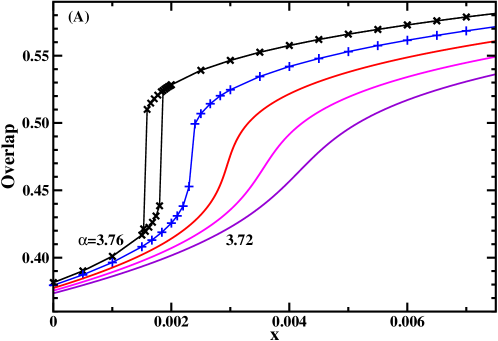
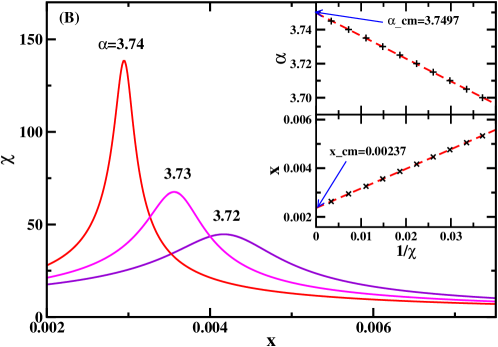
Figure 7: Mean-field predictions on the mean solution-pair overlap $\overline{q}(x)$ (A) and the overlap susceptibility $\chi(x)$ (B) for the random $3$-SAT problem. In (A) the constraint density $\alpha$ increases from $3.72$ to $3.76$ (right to left) with step size $0.01$. The inset of (B) shows how the inverse of the peak value of $\chi(x)$ approaches zero as $\alpha$ increases to $\alpha_{cm}(3)=3.7497$ from below. At $\alpha=\alpha_{cm}$, $\chi(x)$ becomes infinite at $x=x_{cm}(3)=0.00237$.

The overlap susceptibility $\chi(x)$ measures the sensitivity of the mean solution-pair overlap with the coupling field $x$, it is defined by $\chi(x)\equiv{\rm d}\overline{q}(x)/{\rm d}x$. The susceptibility $\chi(x)$ is related to the overlap fluctuation by

$$\chi(x)=\frac{1}{N}\sum\limits_{i=1}^{N}\sum\limits_{j=1}^{N}\left[\langle\sigma_{i}^{1}\sigma_{i}^{2}\sigma_{j}^{1}\sigma_{j}^{2}\rangle_{x}-\langle\sigma_{i}^{1}\sigma_{i}^{2}\rangle_{x}\langle\sigma_{j}^{1}\sigma_{j}^{2}\rangle_{x}\right]\ .$$ (22)

Figure 7(b) demonstrates that, as $\alpha$ approaches $3.75$ from below, the peak value of $\chi(x)$ becomes more and more pronounced and finally diverges. From the divergence of the peak value of $\chi(x)$, we obtain that $\alpha_{cm}(3)=3.7497$ for the random $3$-SAT problem. This value is much below the value of $\alpha_{d}(3)=3.87$.

Similar mean-field calculations are performed for the random $4$-SAT problem and we obtain that $\alpha_{cm}(4)=8.4746$. This value is again much below the clustering transition point $\alpha_{d}(4)=9.38$.

3.2 Dynamical heterogeneity of Glauber dynamics

The solution space heterogeneity of the random $K$-SAT problem influences the dynamics of random walking diffusion processes [6]. Similar to the random $K$-XORSAT problem, we can represent the solution space of the random $K$-SAT problem as a solution graph of nodes and edges, with the nodes denoting individual solutions and the edges connecting pairs of solutions of unit Hamming distance. When the constraint density $\alpha$ of the random $K$-SAT problem is less than $\alpha_{d}(K)$, this solution graph has a single giant connected component that includes almost all the solutions of the solution space. In this ergodic phase of $\alpha<\alpha_{d}(K)$, the structure of this huge solution graph become heterogeneous when the solutions aggregate into many different communities. There are many domains of high edge density in the solution graph, corresponding to the different solution communities. The nodes of different domains are also connected by many edges, but the density of inter-domain edges is much lower than the density of intra-domain edges. As was demonstrated in [6], this heterogeneity of edge density causes an entropic trapping effect to diffusive particles on the solution graph. The dynamics of a diffusive particle can be decomposed into a trapping mode (the particle diffuses within a relatively dense-connected domain of the solution graph) and a transition mode (the particle escapes from one domain of the solution graph, wonders for a while, and then enters into another domain of the solution graph). As the trajectory of the diffusive particle oscillates between the trapping mode and the transition mode, if a clustering analysis is performed on a set of solutions sampled from this trajectory at equal time interval, a clear community structure can be observed among the sampled solutions [6, 8].

The solution space diffusion process can be turned into a stochastic search algorithm. One such algorithms, the SEQSAT of [36], constructs a solution for a random $K$-SAT problem in a sequential manner. Constraints of the problem are added one after another in a random order, and as a new constraint is added, a random walk process of single-spin flips is performed in the solution space of the satisfied sub-problem to reach a solution that also satisfies the new constraint. It was observed [36, 8] that, when the constraint density $\alpha$ of the satisfied sub-problem exceeds $\alpha_{cm}(K)$, the SEQSAT search process becomes viscous, the mean waiting time needed to satisfy a new constraints starts to increases rapidly with $\alpha$, and the sequence of waiting times starts to have large fluctuations. This dynamical behavior is easily understood in terms of the heterogeneity of the underlying solution space.

Solution space structural heterogeneity results in dynamical heterogeneity of diffusion processes. To demonstrate this point more clearly and to estimate a typical relaxation time, we study in this subsection a simple solution space Glauber dynamics. For a large random $K$-SAT problem with $N$ variables and $M=\alpha N$ constraints ($\alpha<\alpha_{d}(K)$), first we construct through SEQSAT a spin configuration that satisfies all the $M$ constraints. (Of cause we can also use other heuristic algorithms to generate an initial solution. The only requirement is that this solution should be a typical solution, or in other words, it should belong to the single largest solution cluster of the solution space. This requirement is satisfied in our simulation studies.) Then we set the initial time as $t=-T_{e}$ and denote the initial solution as $\vec{\sigma}(-T_{e})\equiv(\sigma_{1}(-T_{e}),\sigma_{2}(-T_{e}),\ldots,\sigma_{N}(-T_{e}))$. The spin configuration is then updated by single-spin flips at each elementary time step $\Delta t=1/N$. Let us suppose at time $t$ the spin configuration is $\vec{\sigma}(t)$. Then a vertex $i$ is chosen uniformly randomly from the whole vertex set $\{1,2,\ldots,N\}$; a candidate spin configuration $\vec{\sigma}^{\prime}$ is constructed, with $\sigma_{j}^{\prime}=\sigma_{j}(t)$ if $j\neq i$ and $\sigma_{i}^{\prime}=-\sigma_{i}(t)$. If $\vec{\sigma}^{\prime}$ is not a solution of the $K$-SAT problem, then at time $t^{\prime}=t+\Delta t$, the old spin configuration is kept, i.e., $\vec{\sigma}(t^{\prime})=\vec{\sigma}(t)$. However, if $\vec{\sigma}^{\prime}$ is also a solution, then with probability one-half $\vec{\sigma}(t^{\prime})=\vec{\sigma}(t)$ and with the remaining probability one-half $\vec{\sigma}(t^{\prime})=\vec{\sigma}^{\prime}$.

A unit time of the above-mentioned Glauber dynamics corresponds to $N$ spin-flip attempts. The actual number of accepted spin flips in a unit time is about $0.1N$ for the problem instances of figure 8 and figure 9. If this random walk diffusion process is simulated for an extremely long period of time, every solution in the connected component of the solution graph which the initial solution $\vec{\sigma}(-T_{e})$ belongs will have the same frequency of being visited. The time $T_{e}$ is set to be large enough (e.g., $T_{e}\sim 10^{8}$) to ensure that the diffusion process has completely forget the initial solution $\vec{\sigma}(-T_{e})$ at time $t\geq 0$.

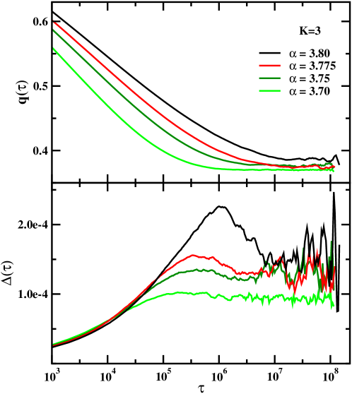
Figure 8: Glauber dynamics simulation results for a single random $K$-SAT ($K=3$) problem instance with $N=10^{5}$ vertices. At a given value of $\alpha$, the first $M=\alpha N$ constraints of this single random instance are used in the simulation. (Upper panel) Mean value of the overlap $q(\tau)$ between two solutions separated by time $\tau$ along the trajectory of configuration evolution. (Lower panel) The variance $\Delta(\tau)$ of the solution-pair overlap $q(\tau)$.

For the trajectory of spin configurations at $t\geq 0$, the quantity $q(\tau)=(1/N)\sum_{i=1}^{N}\sigma_{i}(t)\sigma_{i}(t+\tau)$ measures the overlap between two spin configurations $\vec{\sigma}(t)$ and $\vec{\sigma}(t+\tau)$ that are separated by a time $\tau$. $q(\tau)$ is a random variable, its value fluctuates with different choices of the time $t$. We are mainly interested in the mean value $\overline{q}(\tau)$ and the variance $\Delta(\tau)$ of the overlap $q(\tau)$. The mean overlap $\overline{q}(\tau)$ is calculated by

$$\overline{q}(\tau)\equiv\langle q(\tau)\rangle_{t}=\frac{1}{N}\sum\limits_{i=1}^{N}\langle\sigma_{i}(t)\sigma_{i}(t+\tau)\rangle_{t}\ ,$$ (23)

where $\langle\ldots\rangle_{t}$ means averaging over different starting times $t\geq 0$ along the diffusion trajectory. The variance $\Delta(\tau)$ is expressed as

$$\Delta(\tau)=\frac{1}{N^{2}}\sum_{i=1}^{N}\sum_{j=1}^{N}\left[\langle\sigma_{i}(t)\sigma_{i}(t+\tau)\sigma_{j}(t)\sigma_{j}(t+\tau)\rangle_{t}-\langle\sigma_{i}(t)\sigma_{i}(t+\tau)\rangle_{t}\langle\sigma_{j}(t)\sigma_{j}(t+\tau)\rangle_{t}\right]\ .$$

(24)

Comparing (24) with (22), a dynamical susceptibility $\chi_{4}(\tau)$ can be defined as $\chi_{4}(\tau)\equiv N\Delta(\tau)$ (such a quantity was introduced in [37, 10], see also the review [38]).

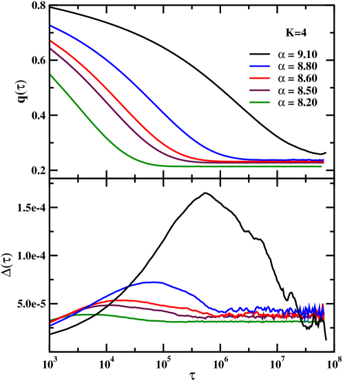
Figure 9: Same as figure 8, but for $K=4$.

The upper panel of figure 8 shows the relaxation behavior of $\overline{q}(\tau)$ for a large random $3$-SAT formula with $N=10^{5}$ vertices. To study how the shape of $\overline{q}(\tau)$ changes with constraint density $\alpha$, the first $M=\alpha N$ constraints of this same formula is used for Glauber dynamics simulation at each value of $\alpha$. We focus on $\alpha$ values in the vicinity of $\alpha_{cm}(3)$. For $\alpha=3.70$, the mean overlap $\overline{q}(\tau)$ reaches its plateau value of $0.37$ at $\tau\approx 10^{6}$. For $\alpha=3.75\simeq\alpha_{cm}(3)$, the plateau of $\overline{q}(\tau)$ is reached at $\tau\approx 10^{6.5}$, and its value increases to $0.38$. For $\alpha=3.80$, the plateau of $\overline{q}(\tau)$ is reached at $\tau\approx 10^{7.2}$, with a value of about $0.39$. These and our other unshown simulation results clearly confirm that, as $\alpha$ exceeds $\alpha_{cm}(3)$, the relaxation of the solution space diffusion process is slowed down greatly.

The lower panel of figure 8 shows the variance $\Delta(\tau)$ of the solution-pair overlap values. At $\alpha=3.70$, the variance $\Delta(\tau)$ increases with $\tau$ and reaches its plateau value at $\tau\approx 10^{6}$. At $\alpha=3.75$, $\Delta(\tau)$ starts to show a peak at $\tau\approx 10^{5.5}$. The peak of $\Delta(\tau)$ becomes more and more pronounced as $\alpha$ further increases, and the time $\tau_{dh}$, corresponding to the peak value of $\Delta(\tau)$, shifts to larger values with $\alpha$. At $\alpha=3.80$, $\tau_{dh}\approx 10^{6}$.

The peak time $\tau_{dh}$ of the variance $\Delta(\tau)$ gives a measure of the typical time scale of dynamical heterogeneity of the Glauber dynamics. For $\tau\ll\tau_{dh}$, two solutions $\vec{\sigma}(t)$ and $\vec{\sigma}(t+\tau)$ have a large chance of being in the same solution community, therefore the fluctuation of overlap values $q(\tau)$ is small; a large fraction of vertices are inactive in this relatively short time window of $\tau$, as their spin values are flipped only with low frequencies. On the other hand, for $\tau\gg\tau_{dh}$, the compared two solutions $\vec{\sigma}(t)$ and $\vec{\sigma}(t+\tau)$ have a large chance of belonging to two different solution communities, and therefore the fluctuation of their overlap values is again small; the spin values of most of the vertices have been flipped many times during such a large time window, and hence dynamical heterogeneity is destroyed. When the time window $\tau$ is comparable to $\tau_{dh}$, the solutions $\vec{\sigma}(t)$ and $\vec{\sigma}(t+\tau)$ have comparable probabilities of being in the same solution community and being in two different communities; this causes relatively large fluctuation of the overlap values. As $\alpha$ increases from $\alpha_{cm}(3)$ further, it takes more time for the diffusion process to escape from a solution community, and the difference between intra- and inter-community overlap values become larger, these two facts make the peak value $\Delta(\tau)$ and the peak time $\tau_{dh}$ both to increase rapidly.

Figure 9 reports the simulation results for a random $4$-SAT problem instance of $N=10^{5}$ vertices and $M=\alpha N$ constraints. Similar to the case of random $3$-SAT, we find that the viscosity of the Glauber dynamics increases rapidly with constraint density $\alpha$. For $\alpha=9.10>\alpha_{cm}(4)$, the mean overlap $q(\tau)$ reaches its plateau value only at a very large value of $\tau\approx 10^{8}$. As demonstrated by the variance $\Delta(\tau)$ of solution-pair overlaps, dynamical heterogeneity become to manifest itself at $\alpha=8.50\simeq\alpha_{cm}(4)$ and it becomes more and more pronounced as $\alpha$ further increases.

Comparing figure 8 and figure 9 we can also notice an important dynamical difference between the random $3$-SAT and the random $4$-SAT case. For the random $4$-SAT system, we observe that the relaxation curve of $\overline{q}(\tau)$ is $`$Z’ form in shape at $\alpha=9.10$ (i.e., $97\%$ of $\alpha_{d}(4)$), with a plateau value of $q\approx 0.7$ at intermediate time intervals $\tau$ before it finally decay to a much lower $q\approx 0.3$ at $\tau\sim 10^{8}$. The peak of the overlap variance $\Delta(\tau)$ corresponds to the time interval $\tau$ at which $\overline{q}$ starts to decay from the larger plateau. However, for the random $3$-SAT system, we find that the curve of $\overline{q}(\tau)$ has a $`$L’ shape even at $\alpha=3.80$ ($98\%$ of $\alpha_{d}(3)$), and at the time when $\Delta(\tau)$ reaches its peak value, the mean overlap $\overline{q}(\tau)$ is already close to its asymptotic value of $\tau\rightarrow\infty$. We suggest that this dynamical difference is a strong reflect of the difference between the community structures of the random $3$-SAT and the general random $K$-SAT problems with $K\geq 4$.

For the random $3$-SAT problem, in the heterogeneity phase of $\alpha_{cm}(3)<\alpha<\alpha_{d}(3)$, the solution space probably is dominated by a sub-exponential number of largest solution communities. Because of this predominance, the mean intra-community solution-pair overlap of each of these dominating communities is only slightly higher than the mean solution-pair overlap of the whole solution space. Then at typical time $\tau_{dh}$ when the diffusive particle jumps between different dominating solution communities, one will not observe much drop in the mean overlap value $\overline{q}$. Such a picture is consistent with the prediction that, at $\alpha>\alpha_{d}(3)$, only a sub-exponential number of solution Gibbs states dominate the solution space [3].

For the random $K$-SAT problem with $K\geq 4$, however, in the range of $\alpha\in(\alpha_{cm}(K),\alpha_{d}(K))$ the solution space probably is contributed mainly by a exponential number of median-sized solution communities. The sub-exponential number of the largest solution communities has only a negligible contribution to the whole solution space and therefore barely influence the dynamics of the diffusive particle. For such a community structure, then the mean intra-community solution-pair overlap will be much larger than the mean solution-pair overlap of the whole solution space, resulting in a change of trend of $\overline{q}(\tau)$ at $\tau\sim\tau_{dh}$. Such a picture for $K\geq 4$ is again consistent with the prediction that, at $\alpha>\alpha_{d}(K)$ the solution space is dominated by an exponential number of median-sized Gibbs states [3].

3.3 Summary for $K$-SAT

In this section, we confirmed that the solution space of the random $K$-SAT problem becomes heterogeneous at $\alpha\geq\alpha_{cm}(K)$ and determined by the replica-symmetric cavity method that $\alpha_{cm}(3)\simeq 3.75$ and $\alpha_{cm}(4)\simeq 8.47$. We demonstrated that the existence of many solution communities in the solution space caused heterogeneous behavior in the dynamics of a solution space diffusion process. The typical time scale of dynamical heterogeneity of this diffusion process is determined by computer simulations.

4 Outlook

A heterogeneity transition was found to occur in the ground-state configuration spaces of two multiple-spin interaction systems, the random $K$-XORSAT problem and the random $K$-SAT problem. We expect that this transition is a general phenomenon that occurs in many other spin glass systems before the ergodicity-breaking transition of the ground-state configuration space. Such a heterogeneity transition is unlikely to be special to the ground-state configuration space but should also be observed as the energy level (or equivalently the temperature $T$) of the configuration space is lowered to certain critical level. If the configuration space of a spin glass system is ergodic but highly heterogeneous at certain temperature $T$, this structural heterogeneity probably will manifest itself through heterogeneous behaviors in various spin relaxation dynamical processes of the system. More deep understanding on the relationship between the phenomenon of dynamical heterogeneity and the structural heterogeneity of the configuration space is very desirable. Such efforts may bring new ways of probing configuration space heterogeneity from observing features of dynamical heterogeneity.

The solution space heterogeneity of the random $K$-SAT problem has been studied analytically only through the replica-symmetric cavity method. However, from the experiences gained on the random $K$-XORSAT problem, we believe the replica-symmetric cavity theory is not sufficient for a heterogeneous solution space. A complete study on the heterogeneity transition of the random $K$-SAT using the 1RSB mean-field cavity theory will be reported in a later paper.

In the case of the random $K$-SAT problem, we have not yet performed a systematic investigation on the scaling behaviors of the peak value of overlap variance (equivalently, the overlap susceptibility $\chi(\tau)$) and the typical time $\tau_{dh}$ of dynamical heterogeneity. Probably both the peak value of $\chi(\tau)$ and the characteristic time $\tau_{dh}$ diverge at the clustering transition point $\alpha=\alpha_{d}(K)$. To get unambiguous results, we need a more efficient protocol of simulating the diffusion dynamics on the solution space.

Simulations results of [6] and [5] indicated that, for the random $3$-SAT and random $4$-SAT problem, the single solution space Gibbs states at $\alpha>\alpha_{d}(K)$ are themselves very heterogeneous in internal structure. To study analytically the heterogeneity of single solution clusters in the ergodicity-breaking phase, however, appears to be a very challenging task. Such kind of investigations may be very valuable for us to understand how the largest solution clusters of the random $K$-SAT problem evolve with constraint density $\alpha$.

Appendix A The 1RSB cavity equations for the random $K$-XORSAT problem

Here we list the technical details of the 1RSB mean-field cavity theory for the random $K$-XORSAT problem as discussed in section 2.4. For a comprehensive description of the 1RSB mean-field theory, the reader is referred to [1, 2, 3, 35].

When there are an exponential number of Gibbs states, the probability $p_{i\rightarrow a}^{+}$ as defined in section 2.3 will be different for different Gibbs states. The distribution of $p_{i\rightarrow a}^{+}$ among all the Gibbs states is denoted by $P_{i\rightarrow a}(p_{i\rightarrow a}^{+})$. We define $\overline{p}_{i\rightarrow a}^{+}$ as the average value of $p_{i\rightarrow a}^{+}$, i.e., $\overline{p}_{i\rightarrow a}^{+}=\int{\rm d}p^{+}P_{i\rightarrow a}(p^{+})p^{+}$. We also define two auxiliary distributions as [2]

$$Q_{i\rightarrow a}^{+}(p_{i\rightarrow a}^{+}|\overline{p}_{i\rightarrow a}^{+}) =\frac{P_{i\rightarrow a}(p_{i\rightarrow a}^{+})p_{i\rightarrow a}^{+}}{\overline{p}_{i\rightarrow a}^{+}}\ ,$$ (25)

$$Q_{i\rightarrow a}^{-}(p_{i\rightarrow a}^{+}|\overline{p}_{i\rightarrow a}^{+}) =\frac{P_{i\rightarrow a}(p_{i\rightarrow a}^{+})(1-p_{i\rightarrow a}^{+})}{(1-\overline{p}_{i\rightarrow a}^{+})}\ .$$ (26)

$Q_{i\rightarrow a}^{+}(p_{i\rightarrow a}|\overline{p}_{i\rightarrow a}^{+})$ is the conditional probability of $p_{i\rightarrow a}^{+}$ given that $\sigma_{i}=+1$. Similarly, $Q_{i\rightarrow a}^{-}(p_{i\rightarrow a}|\overline{p}_{i\rightarrow a}^{+})$ is the conditional probability of $p_{i\rightarrow a}^{+}$ given that $\sigma_{i}=-1$.

At the special case of $m=1$, it can be shown that the iteration equation for $\overline{p}_{i\rightarrow a}^{+}$ has the same form as (13), with the only difference that all the $p_{j\rightarrow b}^{+}$ values are replaced by their corresponding mean $\overline{p}_{j\rightarrow b}^{+}$, i.e., $\overline{p}_{i\rightarrow a}^{+}=\hat{p}(\{\overline{p}_{j\rightarrow b}^{+}\})$ [3]. The iteration equations for the conditional probabilities $Q_{i\rightarrow a}^{+}(p_{i\rightarrow a}^{+}|\overline{p}_{i\rightarrow a}^{+})$ and $Q_{i\rightarrow a}^{-}(p_{i\rightarrow a}^{+}|\overline{p}_{i\rightarrow a}^{+})$ at $m=1$ have the following expression [2, 3]

$$Q_{i\rightarrow a}^{\sigma_{i}}(p_{i\rightarrow a}^{+}|\overline{p}_{i\rightarrow a}^{+})=\prod\limits_{b\in\partial i\backslash a}\left[\sum\limits_{\sigma_{\partial b\backslash i}}w_{b\rightarrow i}^{\sigma_{i}}(\sigma_{\partial b\backslash i})\prod\limits_{j\in\partial b\backslash i}Q_{j\rightarrow b}^{\sigma_{j}}(p_{j\rightarrow b}^{+}|\overline{p}_{j\rightarrow b}^{+})\right]\delta(p_{i\rightarrow a}^{+}-\hat{p}(\{p_{j\rightarrow b}^{+}\}))\ ,$$

(27)

where $\sigma_{\partial b\backslash i}$ denotes a spin configuration for the vertex set $\partial b\backslash i$ of constraint $b$, and

$$w_{b\rightarrow i}^{\sigma_{i}}(\sigma_{\partial b\backslash i})=\frac{\prod\limits_{j\in\partial b\backslash i}\overline{p}_{j\rightarrow b}^{\sigma_{j}}\delta_{\sigma_{i}\prod_{j\in b\backslash i}\sigma_{j}}^{1}}{\sum\limits_{\sigma_{\partial b\backslash i}}\prod\limits_{j\in\partial b\backslash i}\overline{p}_{j\rightarrow b}^{\sigma_{j}}\delta_{\sigma_{i}\prod_{j\in b\backslash i}\sigma_{j}}^{1}}$$ (28)

is the probability of a satisfying spin assignment $\sigma_{\partial b\backslash i}$ for constraint $b$ given the spin value $\sigma_{i}$ of vertex $i$ (the probability $\overline{p}_{j\rightarrow b}^{-}\equiv 1-\overline{p}_{j\rightarrow b}^{+}$ is the mean probability of vertex $j$ taking spin value $\sigma_{j}=-1$ in the absence of constraint $b$).

The cavity iterative equations for $\overline{p}_{i\rightarrow a}^{+}$ and $Q_{i\rightarrow a}^{\sigma_{i}}(p_{i\rightarrow a}^{+}|\overline{p}_{i\rightarrow a}^{+})$ can be solved by the population dynamics technique [1, 21]. We are interested in the solution space property at a fixed value of the overlap value $q$, so in the population dynamics simulation the magnitude of the coupling field $x$ is adjusted from time to time to ensure that the mean overlap value as expressed by (14) with $p_{j\rightarrow a}^{+}$ replaced by $\overline{p}_{j\rightarrow a}^{+}$ is equal to the specified value $q$ (see, e.g., [39, 21]).

The grand free-energy density $g$ of the model system, as defined by $g=(1/N)\ln Z_{1RSB}$, has the following simplified expression at $m=1$:

$$g= \frac{1}{N}\sum\limits_{i=1}^{N}\ln\left(\sum\limits_{\sigma_{i}}e^{x\sigma_{i}}\prod\limits_{a\in\partial i}\frac{1+\sigma_{i}\prod_{j\in\partial a\backslash i}(2\overline{p}_{i\rightarrow a}^{+}-1)}{2}\right)$$ (29)

$$-\frac{1}{N}\sum\limits_{a=1}^{\alpha N}(K-1)\ln\left(\frac{1+\prod_{i\in\partial a}(2\overline{p}_{i\rightarrow a}^{+}-1)}{2}\right)$$

The mean free energy density $\overline{f}$ of a Gibbs state is expressed as

$$\overline{f}=\frac{1}{N}\sum\limits_{i=1}^{N}\overline{\Delta f_{i}}-\frac{1}{N}\sum\limits_{a=1}^{\alpha N}(K-1)\overline{\Delta f_{a}}\ ,$$ (30)

where $\overline{\Delta f_{i}}$ and $\overline{\Delta f_{a}}$ are, respectively, the free energy increase caused by vertex $i$ and constraint $a$. These two free energy increases are expressed by the following expressions at $m=1$:

$$\overline{\Delta f_{i}}= \sum\limits_{\sigma_{i}}\overline{p}_{i}^{\sigma_{i}}\prod\limits_{a\in\partial i}\left[\sum\limits_{\sigma_{\partial a\backslash i}}w_{a\rightarrow i}^{\sigma_{i}}(\sigma_{\partial a\backslash i})\prod\limits_{j\in\partial a\backslash i}Q_{j\rightarrow a}^{\sigma_{j}}(p_{j\rightarrow a}^{+}|\overline{p}_{j\rightarrow a}^{+})\right]\times$$ (31)

$$\ln\left(\sum\limits_{\sigma_{i}}e^{x\sigma_{i}}\prod\limits_{a\in\partial i}\frac{1+\sigma_{i}\prod_{j\in\partial a\backslash i}(2p_{j\rightarrow a}^{+}-1)}{2}\right)\ ,$$

and

$$\overline{\Delta f_{a}}=\sum\limits_{\sigma_{\partial a}}\left[w_{a}(\sigma_{\partial a})\prod\limits_{i\in\partial a}Q_{i\rightarrow a}^{\sigma_{i}}(p_{i\rightarrow a}^{+}|\overline{p}_{i\rightarrow a}^{+})\right]\ln\left(\frac{1+\prod_{i\in\partial a}(2p_{i\rightarrow a}^{+}-1)}{2}\right)\ .$$ (32)

In (31)), $\overline{p}_{i}^{+}$ is expressed as

$$\overline{p}_{i}^{+}==\frac{e^{x}\prod\limits_{a\in\partial i}\left[\frac{1+\prod\limits_{j\in\partial a\backslash i}(2\overline{p}_{j\rightarrow a}^{+}-1)}{2}\right]}{e^{x}\prod\limits_{a\in\partial i}\left[\frac{1+\prod\limits_{j\in\partial a\backslash i}(2\overline{p}_{j\rightarrow a}^{+}-1)}{2}\right]+e^{-x}\prod\limits_{a\in\partial i}\left[\frac{1-\prod\limits_{j\in\partial a\backslash i}(2\overline{p}_{j\rightarrow a}^{+}-1)}{2}\right]}\ ,$$ (33)

and $\overline{p}_{i}^{-}=1-\overline{p}_{i}^{+}$. The probability $w(\sigma_{\partial a})$ in (32) is expressed as

$$w_{a}(\sigma_{\partial a})=\frac{\prod\limits_{i\in\partial a}\overline{p}_{i\rightarrow a}^{\sigma_{i}}\delta_{\prod_{i\in a}\sigma_{i}}^{1}}{\sum\limits_{\sigma_{\partial a}}\prod\limits_{i\in\partial a}\overline{p}_{i\rightarrow a}^{\sigma_{i}}\delta_{\prod_{i\in a}\sigma_{i}}^{1}}\ .$$ (34)

At $m=1$, the complexity $\Sigma$, the total free entropy density $s_{total}$, and the mean entropy density of a solution community, $s_{cm}$, are calculated to be

$$\Sigma= g-\overline{f}\ ,$$ (35)

$$s_{total}= g-xq\ ,$$ (36)

$$s_{cm}= \overline{f}-xq\ .$$ (37)

The equality $s_{total}=s_{cm}+\Sigma$ holds at $m=1$.

It appears that at some overlap values $q$, more than one mean-field 1RSB solutions can be produced by the population dynamics simulation at $m=1$. These different mean-field solutions have the same value of $s_{total}$ but different values of $\Sigma$ and $s_{cm}$. In such a case we choose the mean-field solution with the largest value of $\Sigma$ (similar situations of multiple mean-field solutions were observed earlier in the random $K$-SAT problem at $m<1$ [40, 35]).

References

References

- [1] M. Mézard and G. Parisi. The Bethe lattice spin glass revisited. Eur. Phys. J. B, 20:217–233, 2001.
- [2] M. Mézard and A. Montanari. Reconstruction on trees and spin glass transition. J. Stat. Phys., 124:1317–1350, 2006.
- [3] F. Krzakala, A. Montanari, F. Ricci-Tersenghi, G. Semerjian, and L. Zdeborova. Gibbs states and the set of solutions of random constraint satisfaction problems. Proc. Natl. Acad. Sci. USA, 104:10318–10323, 2007.
- [4] E. Gardner. Spin glasses with -spin interactions. Nucl. Phys. B, 257 [FS14]:747–765, 1985.
- [5] K. Li, H. Ma, and H. Zhou. From one solution of a -satisfiability formula to a solution cluster: Frozen variables and entropy. Phys. Rev. E, 79:031102, 2009.
- [6] H. Zhou and H. Ma. Communities of solutions in single solution clusters of a random -satisfiability formula. Phys. Rev. E, 80:066108, 2009.
- [7] H. Zhou. Criticality and heterogeneity in the solution space of random constraint satisfaction problems. arXiv:0911.4328, 2009; Int. J. Modern Phys. B (in press).
- [8] H. Zhou. Solution space heterogeneity of the random -satisfiability problem: Theory and simulations. J. Phys.: Conf. Series, 233:012011, 2010.
- [9] A. Crisanti and H.-J. Sommers. The spherical -spin interaction spin glass model: the statics. Z. Phys. B, 87:341–354, 1992.
- [10] C. Donati, S. Franz, S. C. Glotzer, and G. Parisi. Theory of non-linear susceptibility and correlation length in glasses and liquids. J. Non-Cryst. Solids, 307-310:215–224, 2002.
- [11] S. Franz and G. Parisi. Recipes for metastable states in spin glasses. J. de Physique I, 5:1401–1415, 1995.
- [12] S. Franz and G. Parisi. Phase diagram of coupled glassy systems: a mean-field study. Phys. Rev. Lett., 79:2486–2489, 1997.
- [13] F. Krzakala and L. Zdeborova. Following Gibbs states adiabatically: The energy landscape of mean field glassy systems. arXiv:0909.3820, 2009.
- [14] L. Zdeborova and F. Krzakala. Generalization of the cavity method for adiabatic evolution of Gibbs states. Phys. Rev. B, 81:224205, 2010.
- [15] F. Ricci-Tersenghi, M. Weigt, and R. Zecchina. Simplest random -satisfiability problem. Phys. Rev. E, 63:026702, 2001.
- [16] M. Mézard, F. Ricci-Tersenghi, and R. Zecchina. Two solutions to diluted -spin models and xorsat problems. J. Stat. Phys., 111:505–533, 2003.
- [17] S. Cocco, O. Dubois, J. Mandler, and R. Monasson. Rigorous decimation-based construction of ground pure states for spin-glass models on random lattices. Phys. Rev. Lett., 90:047205, 2003.
- [18] A. Montanari and G. Semerjian. On the dynamics of the glass transition on bethe lattices. J. Stat. Phys., 124:103–189, 2006.
- [19] A. Montanari and G. Semerjian. Rigorous inequalities between length and time scales in glassy systems. J. Stat. Phys., 125:23–54, 2006.
- [20] N. Sourlas. Spin-glass models as error-correcting codes. Nature, 339:693–695, 1989.
- [21] T. Mora and M. Mézard. Geometrical organization of solutions to random linear boolean equations. J. Stat. Mech.: Theor. Exp., P10007, 2006.
- [22] F. R. Kschischang, B. J. Frey, and H.-A. Loeliger. Factor graphs and the sum-product algorithm. IEEE Trans. Infor. Theor., 47:498–519, 2001.
- [23] M. Mezard and A. Montanari. Information, Physics, and Computation. Oxford Univ. Press, New York, USA, 2009.
- [24] S. Kirkpatrick and B. Selman. Critical behavior in the satisfiability of random boolean expressions. Science, 264:1297–1301, 1994.
- [25] D. Achlioptas. Lower bounds for random -sat via differential equations. Theor. Comput. Sci., 265:159–185, 2001.
- [26] D. Achlioptas, A. Naor, and Y. Peres. Rigorous location of phase transitions in hard optimization problems. Nature, 435:759–764, 2005.
- [27] M. Mézard, T. Mora, and R. Zecchina. Clustering of solutions in the random satisfiability problem. Phys. Rev. Lett., 94:197205, 2005.
- [28] R. Monasson and R. Zecchina. Entropy of the k-satisfiability problem. Phys. Rev. Lett., 76:3881–3885, 1996.
- [29] M. Mézard, G. Parisi, and R. Zecchina. Analytic and algorithmic solution of random satisfiability problems. Science, 297:812–815, 2002.
- [30] M. Mézard and R. Zecchina. The random k-satisfiability problem: from an analytic solution to an efficient algorithm. Phys. Rev. E, 66:056126, 2002.
- [31] G. Semerjian. On the freezing of variables in random constraint satisfaction problems. J. Stat. Phys., 130:251–293, 2008.
- [32] J. Ardelius and L. Zdeborova. Exhaustive enumeration unveils clustering and freezing in the random -satisfiability problem. Phys. Rev. E, 78:040101(R), 2008.
- [33] S. Mertens, M. Mézard, and R. Zecchina. Threshold values of random -sat from the cavity method. Rand. Struct. Algorithms, 28:340–373, 2006.
- [34] H. Zhou. Long-range frustration in finite connectivity spin glasses: a mean-field theory and its application to the random -satisfiability problem. New J. Phys., 7:123, 2005.
- [35] A. Montanari, F. Ricci-Tersenghi, and G. Semerjian. Clusters of solutions and replica symmetry breaking in random -satisfiability. J. Stat. Mech.: Theor. Exper., P04004, 2008.
- [36] H. Zhou. Glassy behavior and jamming of a random walk process for sequentially satisfying a constraint satisfaction formula. Eur. Phys. J. B, 73:617–624, 2010.
- [37] G. Parisi. Short-time aging in binary glasses. J. Phys. A: Math. Gen., 30:L765–L770, 1997.
- [38] A. Cavagna. Supercooled liquids for pedestrians. Phys. Report, 476:51–124, 2009.
- [39] F. Krzakala, F. Ricci-Tersenghi, and L. Zdeborová. Elusive spin-glass phase in the random field Ising model. Phys. Rev. Lett., 104:207208, 2010.
- [40] H. Zhou. mean-field population dynamics approach for the random -satisfiability problem. Phys. Rev. E, 77:066102, 2008.