Long Range Structure of the Nucleon

?abstractname?

The long range structure of the nucleon is discussed starting from the old model of a quark bag with a pion cloud (“cloudy bag”) carrying on to the more recent ideas of the parton model of the nucleon. On the basis of the most recent measurements of the form factors at MAMI, JLab and MIT quantitative results for nucleon charge densities are presented within both non-relativistic and relativistic frameworks.

1 Introduction: Ranges

Many physicists have the following picture of the structure of the nucleon : In the inner region at “short range” reside quarks bound by gluons, in the outer region at “large distances” live mesons and in particular pions. The nucleon consists of constituents, i.e. “constituent quarks” and pions, as the atom consists of a nucleus and electrons, and the nucleus of protons and neutrons. The range of the inner “coloured” region, frequently called “confinement radius”, is rather elusive. It is a model parameter in the old bag model or models for the nucleon resonances based on the constituent quarks. One can estimate it from experiment by identifying it with the “annihilation radius” of the antiproton-proton system. Only quark-antiquark annihilation in the overlap region of colour can contribute to annihilation [1]. It amounts to approximately 0.8 fm, in reasonable agreement with the mentioned model parameters. However, it cannot be easily identified with the root-mean-square (rms) radius of the electric charge of the proton, since the pion cloud will contribute to the charge distribution. A rough idea of the range of this contribution may be gotten by the Compton wave length of the pion which is of the order of 1.4 fm. A similar picture emerges from diffractive scattering of high energy protons and antiprotons [2].

However, this picture fails in two ways. Firstly, the nucleon moves after the scattering in most experiments at relativistic velocities and therefore its structure looks different in different reference frames. The simplest example is the transformation of the magnetic moment into an electric dipole moment. This situation makes it particularly difficult to compare experiments to model calculations based on rest frame wave functions. These wave functions have to be “boosted” to the correct momentum transfer and there is no consistent way of doing that. Secondly, at relativistic energies particle-antiparticle, i.e. quark-antiquark, pairs have unavoidably to be considered making the picture much more involved. These two aspects will be discussed in Section 3.

The relativity destroys the simple picture also in another way. We usually relate ranges with momentum transfer via Heisenberg’s uncertainty relation. However, since in relativistic mechanics space and time are intimately connected no relativistic uncertainty relation exists [3]. Therefore the assignment of ranges to quantities depending on the negative four momentum transfer squared $Q^{2}=-q^{2}$, as e.g. in some plots of the running coupling constant, is rather misleading. We shall, therefore, in this article distinguish between the non-relativistic picture derived at small momentum transfers and the relativistic case where we have to use the relativistic quantum field theoretic description. At small momentum transfers we can approximate the four momentum transfer $q$ with the three momentum transfer $\vec{q}^{\,2}\approx-q^{2}$ and maintain the familiar interpretation of form factors (Section 2). In Section 3 we shall show how we can connect the non-relativistic picture to the underlying quark-gluon structure. We shall see that new experiments in just the relativistic domain are needed in order to clarify how nucleons are made up of quarks and gluons or more precisely how hadrons emerge from QCD.

2 Nonrelativistic interpretation of nucleon form factors

The non-relativistic electromagnetic form factor (FF) is a special case of one of the fundamental observables in quantum mechanics. It is the matrix element of the interaction propagator of the exchange photon, i.e. the operator $e^{i\vec{q}\cdot\vec{r}}$. It appears in all domains of micro physics ranging from atomic physics, the Mössbauer effect to particle physics [4]. It reads in the case of elastic scattering from a charge density $\rho(\vec{r})=\langle\vec{r}|\vec{r}\rangle$

$$F(\vec{q})=\int d^{3}\vec{r}\,\langle\vec{r}\,|\,e^{i\vec{q}\cdot\vec{r}}\,|\,\vec{r}\rangle.$$ (1)

Since we have the idea that the photon interacts with a single constituent we can interpret the form factor as the probability that we scatter from a constituent with a momentum just right to leave the bound system “intact”, i.e. in the ground state. Since one deals mostly with spherically symmetric systems it is customary to write $F(q^{\,2})$.

The method to derive charge and magnetic distributions from the scattering of electro-magnetically interacting particles - almost exclusively these are electrons - has been extensively used for nuclei and nucleons. As a reminder we present the Rosenbluth formula, the key formula connecting the measured cross sections to the FFs for a spin-1/2 particle :

$$\left.\frac{d\sigma}{d\Omega}\right|_{lab}=\underbrace{\left(\frac{\alpha^{2}}{4E^{2}sin^{4}(\theta/2)}\right)}_{\textstyle\sigma_{\text{Mott}}}\frac{E^{\prime}}{E}\\ \times\biggl{\{}\frac{G^{2}_{E}+\tau G^{2}_{M}}{1+\tau}\,cos^{2}(\theta/2)-2\tau G^{2}_{M}\,sin^{2}(\theta/2)\biggr{\}}$$ (2)

where $E$ is the incoming and $E^{\prime}$ the outgoing electron energy, $\theta$ the scattering angle, and $\tau=Q^{2}/(4M^{2})$ with $M$ the mass of the nucleon. Dividing the measured cross section by the Mott cross section, i.e. the cross section for point particles, yields the combination of the quadratic electric form factor $G^{2}_{E}$ and magnetic $G^{2}_{M}$. By varying the scattering angle $\theta$ and the incoming electron energy $E$ in such a way that $Q^{2}$ is constant, $G^{2}_{E}$ and $G^{2}_{M}$ can be separated, the so called Rosenbluth separation. This formula is relativistically correct meaning that the FFs are functions of $Q^{2}$. As a practical tool, the Rosenbluth method is not ideal, however, for very small cross sections as is the case when extracting the small $G^{2}_{E}$ term of the neutron, or when separating at large $Q^{2}$ the small $G^{2}_{E}$ contribution of the proton from that of $G^{2}_{M}$ since the latter dominates at large momentum transfers. Here polarized electrons available with sufficient intensity since about a decade, together with polarized targets or recoil polarimetry, have changed our possibilities dramatically.

In order to give a feeling for the significance of the method we present the example of nuclei. Nuclei are heavy and have in many cases no magnetic contribution, hence the charge distribution can be precisely determined. Figure 1 shows a collection of data for the scattering of electrons from ${}^{16}O$ and ${}^{208}Pb$.

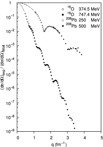
?figurename? 1: A compilation of form factors (FFs) from elastic electron scattering for ${}^{16}O$ and ${}^{208}Pb$ measured at the electron-accelerator laboratories: Amsterdam, Darmstadt, Mainz, Saclay, and Stanford. The FFs have been corrected for the Coulomb distortions different at the electron energies available at these laboratories. The diffraction pattern determining the charge distribution is nicely seen. (From Ref. [5]).

The Fourier transform (see Eq. (1)) of the FFs derived from these cross sections allows for a model independent precise determination of the charge distributions. This is shown in Fig. 2 for some nuclei. These distributions can be well modeled by mean field calculations based on the nuclear shell model [6].

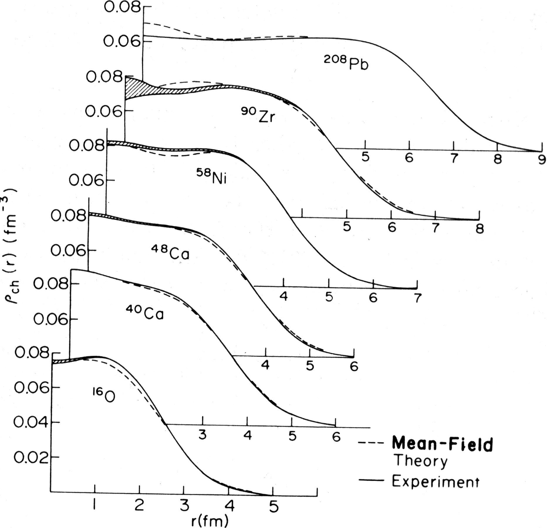
?figurename? 2: Charge distributions of spherical nuclei as derived by model independent analyses from experiment (solid lines). The hatched areas indicate the range of the charge consistent with the data. The dashed lines depict the results of calculations in the framework of nuclear mean-field theory. (From Ref. [6])

We see that the nuclear charge distributions have a subtle structure on top on the bulk behaviour of the saturated nuclear matter. This structure reflects the shell model wave functions and is very sensitive to the details of the nucleon-nucleon interaction but even more importantly to the many body features of the nuclei made up of the constituents protons and neutrons. Only the most sophisticated mean field theories are able to almost reproduce this structure [6]. It remains an unexplained deviation which may be due to too narrow error bands [7].

Let us now turn to the nucleons and see what we know here (see e.g. Refs. [8, 9, 10] for some recent reviews on nucleon form factors). The pre-2000 data suggest that the magnetic and electric form factor of the proton follow a universal form, the “dipole form” $G_{D}(Q^{2})=1/(1+Q^{2}/\Lambda_{D}^{2})^{2}$, with the scale parameter $\Lambda_{D}=0.843$ GeV approximately equal to the mass $m_{\rho}$ of the $\rho$ meson. The case was closed and considered to be text book material. This finding was the basis for the much discussed “vector dominance model” in strong interactions. (For a recent discussion see ref. [11].) The $\rho$ meson mass defines a “small range” of an exponential distribution, somewhat unphysical due to its discontinuity at $r=0$. It was believed that the dipole form would also describe the long ranges characterized by the rms radius of the proton. A measurement at the High Energy Physics Laboratory HEPL at Stanford gave $\sqrt{\langle r^{2}\rangle}=(0.805\pm 0.011)$ fm $\approx\sqrt{12}/m_{\rho}$ [12]. However, as it is now clear, a measurement at Mainz in 1980 [13] which yielded $\sqrt{\langle r^{2}\rangle}=(0.862\pm 0.012)$ fm was closer to the best value $(0.882\pm 0.010)$ fm available today. (For a more detailed discussion see Ref. [14].) This value is confirmed by a recent high precision determination at the Mainz Microtron (MAMI) yielding [7]:

$$\sqrt{\langle r^{2}\rangle}=(0.879\pm 0.005_{\mathrm{stat.}}\pm\\ 0.004_{\mathrm{syst.}}\pm 0.005_{\mathrm{model}})\,\mathrm{fm}.$$ (3)

As discussed in Ref. [14] this value is significantly larger than the largest value derived from dispersion relations and is unexplained in most nucleon models. On the other hand, a recent study of the Lamb shift in muonic hydrogen at the Paul-Scherrer Institute in Zuerich yielded a very precise value as low as $(0.840\pm 0.001)$ fm [15] in agreement with the upper bound of the dispersion-relations calculations. It is not credible to assign this five standard deviation difference to a deficiency in the theory of the electronic experiments which is the same Quantum Electrodynamics as for the muonic hydrogen. However, the calculations of the Lamb shift in muonic hydrogen are difficult due to the strong distortions of the muon wave function calling for further theoretical work.

Considering the focus on “long ranges” the question arises how much of the rms radius is possibly due to a pion cloud. There were weak indications that the pion cloud could be directly seen in the FFs in a similar way as the shell structure of the nucleus. This indication came from a coherent analysis of the data available until 2003 for the electric and magnetic FFs of the proton and neutron [16]. Since 2003 the data base has improved so much that we want to base this discussion on the most recent measurements.

Figure 3 shows the electric FF of the proton as derived from a direct fit of a FF model to data obtained with the 3-Spectrometer set-up at MAMI. This method takes advantage of modern computers and fits Eq. (2) to a large set of angular distributions measured at five energies 180, 370, 450, 720, and 850 MeV. All together about 1400 settings were measured. In this way the “measurement at constant $Q^{2}$”, i.e. the old Rosenbluth separation, becomes obsolete and a very broad kinematic range can be covered indeed. However, since this method is somewhat unfamiliar Fig. 4 shows the best fit curve of Fig. 3 together with the results at those kinematics at which a traditional Rosenbluth separation could be done. The agreement is very good. A point of concern may be the analytical model used for the electric form factor $G_{Ep}$ and magnetic form factor $G_{Mp}$ in the direct FF fits. Here about a dozen different forms have been used all yielding essentially the same results [7]. The rms radius is, however, somewhat dependent on them and the second systematic error in Eq. (3) reflects this dependence.

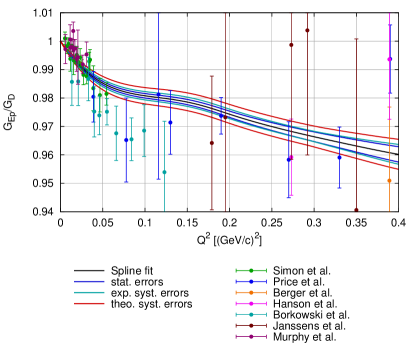
?figurename? 3: The electric FF of the proton $G_{Ep}/G_{D}$ obtained from a direct fit to the cross sections with the spline model to data measured with the 3-Spectrometer set-up at MAMI. The FF is normalised to the dipole form given in the text. The 1 $\sigma$-error band is shown for the indicated errors. In order to show the improvement, the old data obtained with the classical Rosenbluth separation are also depicted.

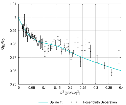
?figurename? 4: As Fig. 3 without error bands but with the results from the classical Rosenbluth separation of the new MAMI data.

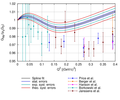
?figurename? 5: As Fig. 3 for the magnetic FF $G_{Mp}/(\mu_{p}G_{D})$ of the proton.

It is evident that these form factors show some structure after the gross dependence, assumed to be given by the standard dipole form, has been divided out. In Fig. 3 one observes two slopes for $G_{E}/G_{D}$. The steep negative slope at small $Q^{2}$ is reflected in the large rms radius discussed above. The reverse is true in Fig. 5 for the rms radius of $G_{M}/(\mu_{p}G_{D})$. A shoulder structure is indicated in both FFs at $Q^{2}\approx 0.15\,\mathrm{GeV}^{2}$. It is shifted compared to the bump structure derived by Friedrich and Walcher [16] from the pre-2003 data and cannot be identified with it. However, just considering the scale of the rms radius and the scale of the structure it is suggestive to look for pion cloud contributions in the modelling of the nucleon.

Since the bulk charge of the proton resides at “small ranges” and extends out to the range of the pion cloud, the separation of the inner component from the pion cloud contribution will be somewhat arbitrary. Here the neutron with a total zero bulk charge promises an experimental access since one way the neutron could acquire a charge distribution is just by its virtual dissociation $n\rightarrow p+\pi^{-}$. This means that the pion cloud should be more clearly visible again as a signal at large radii $r\approx\lambda_{Compton}=1/m_{\pi}\approx 1.4\,$fm in the neutron charge distribution.

One could be tempted to look at the neutron rms radius as in the case of the proton in first place. However, the mentioned recoil effect causes the magnetic moment to contribute to the small electric form factor. It turns out that the electric rms radius of the neutron is a subtle interplay between the recoil effect and the charge radius proper. We do not want to elaborate this here. A summary can be found in Ref. [14]. Instead we will show the most recent results for the electric FF of the neutron.

Figure 6 shows a compilation of all data including the results from the MIT Bates measurement with the BLAST detector at the South Hall Ring at small $Q^{2}$ [18] and the measurement at the Jefferson Laboratory (JLab) by the Hall A Collaboration at large $Q^{2}$ [19]. All these measurements use the dependence of the cross sections of polarized targets or recoil polarizations of the ejected nucleons for polarized electrons from the FFs. The curve shows a fit of the phenomenological model of Friedrich and Walcher (FW) [16].

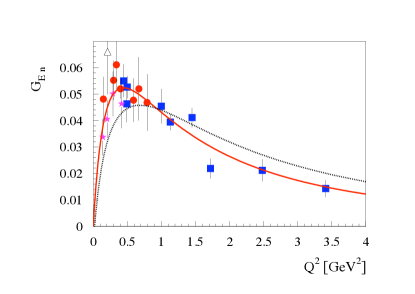
?figurename? 6: A compilation of the recent data for the neutron electric FF, $G_{En}$, obtained at NIKHEF (triangle), Bates MIT (stars), JLab (squares), and MAMI Mainz (circles), with the quasi free $\vec{e}\,d\rightarrow p\,\vec{n}\,e$ and the $\vec{e}\,\overrightarrow{{}^{3}He}\rightarrow pp\,n\,e$ reactions. Either the polarization of the recoiling neutron $\vec{n}$ is measured or the target $\overrightarrow{{}^{3}He}$, and with it the neutron, is polarized. The protons $p$ and $pp$ are unobserved, respectively. The curves correspond with a new fit of a phenomenological model (solid red curve) [16], and of a Generalized Parton Distribution parametrization (dotted black curve) [17].

As already mentioned, the phenomenological FW model tried a coherent fit of a smooth bulk curve with a superimposed bump for the pion cloud. This fit of the before 2003 data showed indeed a $2\,\sigma$ contribution above the smooth curve causing a shift of the negative charge to radii around 1.5 fm. The inclusion of the MIT [18] and JLab data [19] in the fit makes the bump disappear. At small $Q^{2}$ the neutron FFs cannot be reliably determined due to the model dependence of the extraction of the form factor from the scattering of the polarized electrons from unavoidably bound neutrons in deuterium or ³He targets. Only new even more precise measurements will be able to improve the situation. However, it will be mandatory to further study the reaction mechanism experimentally in order to check the theoretical corrections.

The scope of this article is on “long range structure” meaning that one wants to discuss the idea of the spatial distribution of the constituents of the nucleon. In the rest frame the three-dimensional charge distribution of a spherically symmetric non-relativistic system is obtained as :

$$\rho_{3d}(r) = \int_{0}^{+\infty}\frac{dk}{2\pi^{2}}\,k^{2}\,j_{0}(rk)\,\tilde{\rho}(k),$$ (4)

where $\tilde{\rho}(k)$ is an intrinsic FF. As already pointed out the relativistic effects do not allow for a simple interpretation of the electric and magnetic FFs in terms of charge and magnetic density distributions in the rest frame system. However, there is special reference system, the Breit or brick-wall system, defined by having no energy transfer $\nu$ to the nucleon, in which the charge operator for a non-relativistic (static) system is only expressed through the electric FF $G_{E}$. In this system the four-momentum transfer squared becomes $q^{2}=\nu^{2}-\vec{q}^{\,2}=-\vec{q}^{\,2}$. However, the rest frame systems (laboratory systems) for different $q^{2}$ move with different velocities with respect to the Breit system. For a relativistic reference system, to relate its intrinsic FF $\tilde{\rho}(k)$ and density to the Breit frame in which the system of mass $M$ moves with velocity $v=\sqrt{\tau/(1+\tau)}$, requires a Lorentz boost relating $k^{2}=Q^{2}/(1+\tau)$. This relation shows that for $Q^{2}\to\infty$, there is a limiting largest intrinsic wave vector $k\to 2M=2\pi/\lambda_{lim}$. In the rest frame, no information can be obtained on distance scales smaller than this wavelength due to relativistic position fluctuations (known as the Zitterbewegung). For a non-relativistic system as ${}^{16}O$, displayed in Fig. 2, $\lambda_{lim}$ is below 0.04 fm, whereas for the nucleon, it corresponds with $\lambda_{lim}\simeq 0.66$ fm. Extracting the density for a relativistic system as the nucleon, therefore requires a prescription in order to relate the intrinsic FFs $\tilde{\rho}(k)$ in Eq. (4) to the experimentally measured FFs. As an example, in Ref. [20], the prescription $\tilde{\rho}(k)=(1+\tau)^{n}G_{E}(Q^{2})$ motivated by simple models of nucleon structure was used and parameter values $n=0,1$, and 2 were investigated. To see the transitional region from the distance scales where relativistic position fluctuations hamper our extraction of rest frame densities to distances where the concepts of a non-relativistic many-body system can be approximately applied, we visualize the charge density in Fig. 7. It depicts the Fourier transform Eq. (4) using the fit in Fig. 6 (solid red curve). One notices a negative charge density at distances around and larger than 1 fm. With all caveats we may interpret the negative charge as a “pion cloud” in the nonrelativistic limit since it extends beyond the confinement radius of about 0.8 fm.

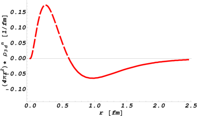
?figurename? 7: Charge distribution of the neutron as derived from the Fourier transform of the $G_{En}$ fit (solid red curve in Fig. 6). The dashed part of the curve is for $r<\lambda_{lim}=2\pi/(2M)$, where one is intrinsically limited to resolve the density due to the Zitterbewegung of the nucleon.

3 Relativistic picture

We now turn to the relativistic picture and see how it does complicate matters, however, for the benefit of a deeper insight. As already mentioned both, the size and the shape of an object, are not relativistically invariant quantities: observers in different frames will infer different magnitudes for these quantities. Furthermore when special relativity is written in a covariant formulation, the density appears as the time component (zero component) of a four-current density $J^{\mu}=(\rho,\textbf{J})$ (in units in which the speed of light $c=1$).

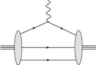
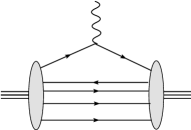
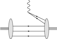
?figurename? 8: Coupling of a space-like photon to a relativistic many-body system, such as the proton. Top panel (a) : diagonal transition where the photon couples to a quark in the leading $3q$ Fock component of the proton. Middle panel (b) : diagonal transition where the photon couples to a quark in a higher Fock component (here $4q\bar{q}$) of the proton. Lower panel (c) : process where the photon creates a $q\bar{q}$ pair leading to a non-diagonal transition between an initial $3q$ state and a final $4q\,\bar{q}$ state.

Besides the relativistic kinematic effects, as e.g. the length contraction, the concept of size and shape in relativistic quantum systems, such as hadrons, is also profoundly modified as the number of degrees of freedom is not fixed anymore. In relativistic quantum mechanics the number of constituents of a system is not constant as a result of virtual pair production. We consider as an example a hadron such as the proton which is probed by a space-like virtual photon, as shown in Fig. 8. A relativistic bound state as the proton is made up of almost massless quarks. Its three valence quarks making up for the proton quantum numbers, constitute only a few percent of the total proton mass. In such a system, the wave function contains, besides the three valence quark Fock component $|qqq\rangle$, also components where additional $q\bar{q}$ pairs, the so-called sea-quarks, and (transverse) gluons $g$ contribute leading to an infinite tower of $|qqqq\bar{q}\rangle$, $|qqqg\rangle$, … components. When probing such a system using electron scattering, the exchanged virtual photon will couple to both kind of quarks, valence and sea, as shown in Figs. 8 (a) and (b). In addition, the virtual photon, can also split into a $q\bar{q}$ pair, leading to a transition from a $3q$ state in the initial wave function to a $4q\bar{q}$ state in the final wave function, as depicted in Fig. 8 (c). Such processes representing non-diagonal overlaps between initial and final wave functions are not positive definite and do not allow for a simple probability interpretation of the density $\rho$ anymore. Only the processes shown in Figs. 8 (a) and (b), with the same initial and final wave function yield a positive definite particle density allowing for a probability interpretation.

This relativistic dynamic effect of pair creation or annihilation fundamentally hampers the interpretation of density and any discussion of size and shape of a relativistic quantum system. Therefore, an interpretation in terms of the concept of a density requires suppressing the contributions shown in Fig. 8 (c). This is possible when viewing the hadron from a light front reference frame allowing for a description of the hadron state by an infinite tower of light-front wave functions [21]. Consider the electromagnetic (e.m.) transition from an initial hadron (with four-momentum $p$) to a final hadron (with four-momentum $p^{\prime}$) viewed from a light-front moving towards the hadron. Equivalently, this corresponds to a frame where the hadrons have a large momentum-component along the $z$-axis chosen along the direction of the hadrons average momentum $P=(p+p^{\prime})/2$. One then defines the light-front plus (+) component by $a^{+}\equiv a^{0}+a^{3}$, in a general four-vector $a^{\mu}$, which is always a positive quantity for both quark or anti-quark four-momenta in the hadron. When we now view the hadron in a so-called Drell-Yan frame [22], where the virtual photon four-momentum $q$ satisfies $q^{+}=0$, energy-momentum conservation will forbid processes in which this virtual photon splits into a $q\bar{q}$ pair. Such a choice is possible for a space-like virtual photon, and its four-momentum or “virtuality” is then given by $q^{2}=-{\vec{q}_{\perp}}^{\,2}\equiv-Q^{2}<0$, where $\vec{q}_{\perp}$ is the transverse photon momentum lying in the $xy$-plane. In such a frame, the virtual photon only couples to forward moving partons, i.e. only processes such as in Fig. 8 (a) and (b) are allowed. We can then define a proper density operator through the + component of the four-current by $J^{+}=J^{0}+J^{3}$ [23]. For quarks it is given by

$$J^{+}=\bar{q}\gamma^{+}q=2q_{+}^{\dagger}q_{+}^{\phantom{\dagger}},\quad\mathrm{with}\quad q_{+}\equiv\frac{1}{4}\gamma^{-}\gamma^{+}q,$$ (5)

where we introduced the $q_{+}$ fields through a field redefinition from the initial quark fields $q$ involving the $\pm$ components of the Dirac gamma matrices. The relativistic density operator $J^{+}$, as defined in Eq. (5), is a positive definite quantity. For systems consisting of e.g. light $u$ and $d$ quarks, multiplying this current with the quark charges yields a quark charge density operator given by $J^{+}(0)=+2/3\,\bar{u}(0)\gamma^{+}u(0)-1/3\,\bar{d}(0)\gamma^{+}(0)d(0)$. Using this charge density operator, one can then define quark (transverse) charge densities in a hadron as [24, 25]:

$$\rho_{0}(b)\equiv\int\frac{d^{2}\vec{q}_{\perp}}{(2\pi)^{2}}\,e^{-i\,\vec{q}_{\perp}\cdot\vec{b}}\,\frac{1}{2P^{+}}\\ \times\langle P^{+},\frac{\vec{q}_{\perp}}{2},+\frac{1}{2}\,|\,J^{+}(0)\,|\,P^{+},-\frac{\vec{q}_{\perp}}{2},+\frac{1}{2}\rangle,$$ (6)

where the hadron is in a state of definite (light-front) helicity. In the two-dimensional Fourier transform of Eq. (6), the two-dimensional vector $\vec{b}$ denotes the quark position in the $xy$-plane relative to the position of the transverse centre-of-momentum of the hadron. It represents the position variable conjugate to the hadron relative transverse momentum which equals just the photon momentum $\vec{q}_{\perp}$.

The quantity $\rho_{0}(b)$ has the interpretation of the two-dimensional unpolarized quark charge density at a distance $b=|\vec{b}|$ from the origin of the transverse c.m. system of the hadron. In the light-front frame, it corresponds to the projection of the charge density in the hadron along the line-of-sight. It is important to mind this difference to the interpretation in the non-relativistic case.

The quark charge density in Eq. (6) does not fully describe the e.m. structure of the hadron, because we know that there are two independent e.m. FFs describing the structure of the nucleon. In general, a particle of spin $S$ is described by $(2S+1)$ e.m. moments. In order to fully describe the relativistic structure of a hadron one needs to consider additionally the charge densities in a transversely polarized hadron state yielding a transverse charge distribution $\rho_{T\,s_{\perp}}$. We denote the transverse polarization direction by $\vec{S}_{\perp}=\cos\phi_{S}\,\hat{e}_{x}+\sin\phi_{S}\,\hat{e}_{y}$. The transverse charge densities can then be defined through matrix elements of the density operator $J^{+}$ in eigenstates of transverse spin as [26, 27, 28]:

$$\rho_{T\,s_{\perp}}(\vec{b})\equiv\int\frac{d^{2}\vec{q}_{\perp}}{(2\pi)^{2}}\,e^{-i\,\vec{q}_{\perp}\cdot\vec{b}}\,\frac{1}{2P^{+}}\\ \times\langle P^{+},\frac{\vec{q}_{\perp}}{2},s_{\perp}|J^{+}|P^{+},\frac{-\vec{q}_{\perp}}{2},s_{\perp}\rangle,$$ (7)

where $s_{\perp}$ is the hadron spin projection along the direction of $\vec{S}_{\perp}$. Whereas the density $\rho_{\lambda}$ for a hadron in a state of definite helicity is circular symmetric for all spins, the density $\rho_{T\,s_{\perp}}$ depends also on the orientation of the position vector $\vec{b}$, relative to the transverse spin vector $\vec{S}_{\perp}$. Therefore, it contains the information on the hadron shape, again projected on the plane perpendicular to the line-of-sight.

The light-front wave functions and light-front densities discussed above are defined at equal light-front time ($x^{+}=0$) of their constituents. When constituents move non-relativistically, it does not make a difference whether they are observed at equal time ($t=0$) or equal light-front time ($x^{+}=0$), since the constituents can only move a negligible small distance during the small time interval that a light-ray needs to connect them. This is not the case, however, for bound systems of relativistic constituents such as hadrons, or even when considering bound systems of non-relativistic constituents if the reference system moves relativistically. Considering the latter, one may ask, for example, how the equal-time wave functions of bound state systems such as the hydrogen atom or positronium, which are non-relativistic bound states in QED at leading order in the fine structure constant $\alpha$, transform when they move relativistically [29, 30]. The case of positronium has been studied in Ref. [29], by using the exact Bethe-Salpeter equation. It was found that the equal-time wave function of its leading $|e^{+}e^{-}\rangle$ Fock state contracts as expected from classical relativity. However, calculating the bound state in relativistic motion also necessitates the inclusion of an $|e^{+}e^{-}\gamma\rangle$ component in the wave function, whose probability is of order $O(\alpha)$. Unlike classical transformation laws, it was found that this photon amplitude, which can be considered as a quantum fluctuation, does not contract [29]. Therefore, the Fock components have a more complex shape change than just a flattening of their distributions along the direction of the boost. Only very recently, relativistic bound states, such as $q\bar{q}$ states in QCD have also been studied at lowest order in $\hbar$ [30]. It was found that the resulting equal-time wave functions have unique Lorentz transformation properties, ensuring the correct dependence of the bound state energy on the center-of-mass momentum. A full understanding of the boost properties of bound state wave functions would allow to relate rest frame densities with light-front densities. For a relativistic many body system as a nucleon, for which this problem still needs to be fully solved theoretically, light-front densities provide at present a consistent theoretical method to image the charge density of quarks. Such imaging is analogous to a flash photograph where different parts of the exposed object are reached by the light ray at different times.

As summarized in the previous section, e.m. FFs of the nucleon are well measured experimental quantities. We will, therefore, discuss the relativistic spatial shape as derived from these FFs. For a nucleon in a state of definite helicity, the transverse quark charge density is obtained from Eq. (6) by taking the two-dimensional Fourier transform of its Dirac FF $F_{1}=(G_{E}+\tau G_{M})/(1+\tau)$ as [24, 25]:

$$\rho_{0}(b)=\int_{0}^{\infty}\frac{dQ}{2\pi}Q\,J_{0}(b\,Q)F_{1}(Q^{2}),$$ (8)

where $J_{n}$ denotes the cylindrical Bessel function of order $n$. Note that $\rho_{0}$ only depends on $b=|\vec{b}|$.

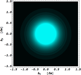
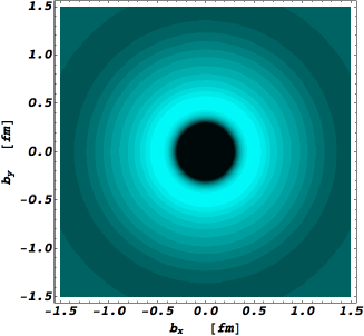
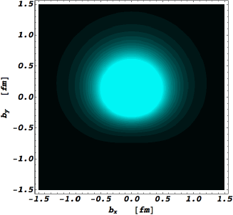
?figurename? 9: Quark transverse charge densities in the proton (left panels) and neutron (right panels). The upper panels show the density in the transverse plane for a nucleon with definite helicity. The lower panels for a nucleon polarized along the $x$-axis. The light (dark) regions correspond with largest (smallest) values of the density. For the proton e.m. FFs, the empirical parametrization of Arrington et al. [32] is used. For the neutron e.m. FFs, the empirical parametrization of Bradford et al. [33] is used.

On the other hand, the information encoded in the Pauli FF $F_{2}=(G_{M}-G_{E})/(1+\tau)$ is connected to a nucleon in a transverse spin state. For a nucleon polarized along the positive $x$-axis, the transverse spin state can be expressed in terms of the light front helicity spinor states by : $|s_{\perp}=+1/2\rangle=\left(|\lambda=+1/2\rangle+e^{i\phi_{S}}\,|\lambda=-1/2\rangle\right)/\sqrt{2}$. The Fourier transform of the expression given in Eq. (7) in a state of transverse spin $s_{\perp}=+1/2$ then yields [26]

$$\rho_{T\frac{1}{2}}(\vec{b})=\rho_{\lambda}(b)\\ \quad+\sin(\phi_{b}-\phi_{S})\,\int_{0}^{\infty}\frac{dQ}{2\pi}\frac{Q^{2}}{2M_{N}}\,J_{1}(b\,Q)F_{2}(Q^{2}).$$ (9)

The second term, which describes the deviation from the circular symmetric unpolarized charge density, depends on the orientation of the transverse position vector $\vec{b}=b(\cos\phi_{b}\hat{e}_{x}+\sin\phi_{b}\hat{e}_{y})$, relative to the transverse spin direction.

In Fig. 9, the transverse charge densities in a nucleon, polarized transversely along the $x$-axis, i.e. for $\phi_{S}=0$, are extracted based on the empirical information on the nucleon e.m. FFs which, however, does not yet contain the most recent data presented in Section 2. For the proton e.m. FFs, the empirical parametrization of Ref. [32] is used, whereas for the neutron e.m. FFs, the empirical parametrization of Ref. [33] is taken. One notices from Fig. 9 that polarizing the proton along the $x$-axis leads to an induced electric dipole moment along the positive $y$-axis equivalent to the anomalous magnetic moment $\mu_{N}$. This field pattern due to the induced electric dipole is a consequence of special relativity. The nucleon spin along the $x$-axis is the source of a magnetic dipole field $\vec{B}$. An observer moving towards the nucleon with velocity $\vec{v}$ will see an electric dipole field pattern with $\vec{E}^{\prime}=-\gamma(\vec{v}\times\vec{B})$ giving rise to the observed asymmetry.

For the neutron, one notices its charge density gets displaced significantly due to its large negative anomalous magnetic moment $\mu_{N}=-1.91$ yielding an induced electric dipole moment along the negative $y$-axis.

To see the impact of the most recent data, presented in Section 2, we compare in Fig. 10 the new data of Bernauer et al. [7] with the previous parametrization of world data, as performed by Arrington et al. [32]. In order to extract charge densities, one requires a form factor parametrization over all values of $Q^{2}$. Because the Bernauer et al. data only provide a precision measurement of $G_{Ep}$ and $G_{Mp}$ for $Q^{2}\leq 0.4$ GeV², to fully quantify their impact on quark charge densities requires a new global analysis combining the previous data with these new data. Here we will perform a first estimate of this by using a parametrization which smoothly connects the new high precision data at low $Q^{2}$ and the Arrington et al. [32] parametrization at larger $Q^{2}$. This interpolation function is displayed in Fig. 10, and is used to extract the two-dimensional quark charge density in a proton in Fig. 11. One readily sees that the new high precision data have a direct impact on the extracted charge densities at large distances, typically larger than about 1.5 fm. By comparing the extracted density, using the previous fit to world data with the new fit, one sees that the new data lead to a significant reduction of the densities at distances larger than about 2 fm. This is a direct consequence of the flatter behavior in $Q^{2}$, for $Q^{2}\leq 0.3$ GeV², which the new data display for both $G_{Ep}$ and $G_{Mp}$.

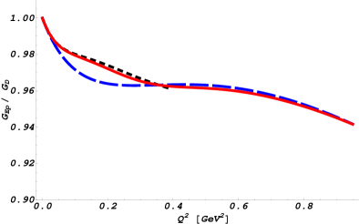
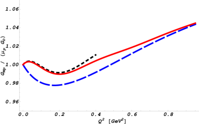
?figurename? 10: Fits to the proton electric (upper panel) and magnetic (lower panel) FFs. Blue (dashed) curve: Arrington et al. [32], black (dotted) curve: Bernauer et al. [7] (only up to $Q^{2}=0.4$ GeV²). The red curve presents a smooth connection between the Bernauer fit at low $Q^{2}$ and the Arrington et al. fit at larger $Q^{2}$.

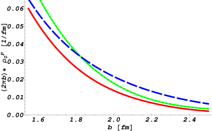
?figurename? 11: Large distance behavior of the unpolarized quark transverse charge density in the proton. The dashed blue curve uses the Arrington et al. parametrization [32]. The solid red curve shows the impact of recent high precision data at low $Q^{2}$ by using a smooth connection between the Bernauer et al. [7] fit at low $Q^{2}$ and the Arrington et al. fit at larger $Q^{2}$ (see solid red curves in Fig. 10). For comparison, the solid green curve is the 2-dimensional projection of the static charge distribution according to Eq. (10), using the interpolating fit for $G_{Ep}$ (red curve in top panel of Fig. 10).

In Fig. 12, we show the corresponding large distance behavior of the quark charge density in the neutron. The transition between the dashed blue curve and the solid red curve in Fig. 12 shows the impact of recent precision data at low $Q^{2}$ for the neutron FFs. These lead to a sizable enhancement in the extracted densities at distances larger than 1.5 fm. It is also of interest to compare these light-front densities with the static densities as discussed in section 2. For a non-relativistic system, one can extract from the 3-dimensional static density of Eq. (4), with intrinsic form factor $\tilde{\rho}(k)=G_{E}(k^{2})$, a 2-dimensional static density as :

$$\rho_{2d}(b) = \int_{-\infty}^{+\infty}dz\,\rho_{3d}(\sqrt{b^{2}+z^{2}}),$$ (10)

$$= \int_{0}^{+\infty}\frac{dQ}{2\pi}\,Q\,J_{0}(bQ)\,G_{E}(Q^{2}).$$

One notices that this static 2-dimensional density has the same form as the light-front density, see Eq. (8), with the crucial difference that in the static density the Sachs electric FF $G_{E}$ appears, whereas for a relativistic system, the proper light-front charge density involves the Dirac FF $F_{1}$. Since the large distance behavior is mostly impacted by the low $Q^{2}$ data, where $G_{E}$ is dominated by $F_{1}$, one expects a qualitatively similar behavior at large distances between both pictures. This is illustrated in Figs. 11 and 12 where the light-front densities (solid red curves) are depicted along with the 2-dimensional static densities (dotted black curves). One notices that for the proton, both densities approach each other at large distances pointing to a large tail in the charge distribution. The corresponding picture for the neutron shows that both light-front and static densities display a negative charge density for distances larger than about 1.6 fm, which can be associated with a negative pion cloud in the outer region of the neutron.

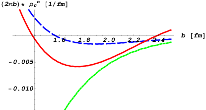
?figurename? 12: Large distance behavior of the unpolarized quark transverse charge density in the neutron. The dashed blue curve is the smooth part of the Friedrich-Walcher parametrization [16]. The solid red curve is the updated Friedrich-Walcher parametrization which includes the recent neutron FF data at low $Q^{2}$. For comparison, the solid green curve is the 2-dimensional projection of the static charge distribution according to Eq. (10), using the most recent fit for $G_{En}$.

A combination of the FF data for the proton and neutron allows to perform a quark flavor separation and map out the spatial dependence of up and down quarks separately. The flavor separated FFs, invoking isospin symmetry, are defined as

$$F_{1,2\;u} = 2F_{1,2\;p}+F_{1,2\;n},$$

$$F_{1,2\;d} = F_{1,2\;p}+2F_{1,2\;n}.$$ (11)

For the Pauli FFs, it is convenient to divide out the normalizations at $Q^{2}=0$, given by the anomalous magnetic moments $\kappa_{u}=2\kappa_{p}+\kappa_{n}$, $\kappa_{d}=\kappa_{p}+2\kappa_{n}$.

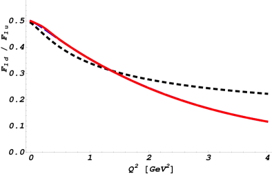
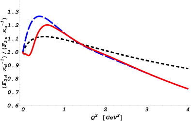
?figurename? 13: Ratio of down/up quark Dirac (upper panel) and Pauli (lower panel) FFs. For the Pauli FFs, the anomalous magnetic moments have been divided out. The dashed blue curves represent a previous fit to world data, whereas the solid red curves shows the impact of recent high precision data at low $Q^{2}$ as described in the text. The dotted black curves represent the results of a Generalized Parton Distribution parametrization [17] of up and down quarks.

We show the ratio of down/up flavor FFs in Fig. 13 and compare two empirical parametrizations with the result of a Generalized Parton Distribution parametrization of up and down quarks. For the empirical parametrizations, the dashed blue curves in Fig. 13 represent a previous fit to world data, using the proton fit of Ref. [32] (dashed blue curve of Fig. 10) and the dipole type neutron fit of the Friedrich Walcher parametrization [16] (solid red curve in Fig. 6). The solid red curve in Fig. 13 shows the impact of recent data at low $Q^{2}$ both for the proton [7] (solid red curve in Fig. 10), as well as the updated Friedrich-Walcher parametrization [16] for the neutron electric and magnetic FFs. One clearly sees from Fig. 13 that the down quark flavor FFs have a faster fall-off than the up quark flavor ones. In the phenomenological GPD parametrizations this is encoded through a down-quark distribution which drops faster at large momentum fractions $x$ than the up-quark distribution. Using Eq. (8), we can then extract the ratio of up/down quark densities in the nucleon, which is displayed in Fig. 14. If the down and up quarks would have the same spatial distribution in the nucleon, the ratio as displayed in Fig. 14 would be one. We see however that in the center region of the proton, at distances smaller than about 0.5 fm, down quarks are less abundant than up quarks. The down quarks have a much wider distribution and are shifted to larger distances, dominating over up quarks between 0.5 to 1.5 fm. At large distances, larger than about 1.5 fm, one clearly sees the impact of the recent data which results in a factor 2 change in the density as compared to previous fits to world data. Although the contribution of the large distance region to the total charge is very small, the new data allow to precisely map out the charge densities in the region well beyond the confinement radius, where the charge density can in turn be interpreted as a measure of the contribution of the pion cloud.

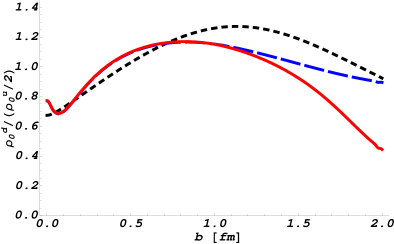
?figurename? 14: Ratio of down over up quark densities in the proton according to the parametrizations and curve conventions of Fig. 13.

4 Conclusion

We have presented two ideas about the long range structure of the nucleon. The first is nonrelativistic in terms of a “bare nucleon” plus a pion cloud, and the second relativistic in terms of quarks and gluons. One may be tempted to believe that the second is more fundamental since it uses the elementary fields of the standard model of particle physics. The quantum theory of quarks and gluons, QCD, describes a very large domain of strong interaction physics indeed. However, at sufficiently low energies, hadrons may be described by effective field theories formulated in terms of fields with discrete quantum numbers. These fields may be viewed as elementary in a certain domain of validity, i.e. sufficiently low energies here. One prominent example of such an effective field is just the pion in Chiral Perturbation Theory emerging as the Goldstone Boson of the spontaneous breaking of chiral symmetry of QCD.

In fact, we are not able to devise a quantitative description of the nucleon-nucleon force in terms of quarks and gluons. On the other hand, the meson exchange idea allows for a very precise description of this force. Therefore, it may be futile to ask the question which description is more correct. Frequently in physics we have to be content with a model allowing a description in a limited domain and, following from this, limited predictive power.

This sometimes confusing situation is also revealed by the two extreme reference frames in which we have considered the structure of the nucleon: the brick-wall system implying an infinitely heavy nucleon and the light-front frame implying a nucleon moving with approximately the speed of light. As we demonstrated in both frames, the long distance structure of the nucleon reflects the physics of the pion cloud. With the recent experimental and theoretical advances we may have come closer to a common picture. However, whether we will ever be able to devise a “final theory” in terms of the elementary fields is an open question. Actually most physics is understood in terms of emergent effective degrees of freedom as the examples of condensed matter physics and nuclear physics show overwhelmingly.

- [1] B. Povh and Th. Walcher, Comments Nucl. Part. Phys. 16 (1986) 85.
- [2] M. Islam, J. Kaspar, R. Luddy, and A. Prokudin, CERN Courier, 49.10 (December 2009) 35.
- [3] L.D. Landau and E.M. Lifshitz, Course of Theoretical Physics, Vol. IV “Quantum Electrodynamics,” by W.B. Berestetskii, E.M. Lifshitz, and L.P. Pitaewskii, Butterworth-Heinemann, Reed-Elsevier Group, Oxford (1971).
- [4] H.L. Lipkin, Quantum Mechanics, New approaches to selected problems. North-Holland Publishing Company, Amsterdam (1973).
- [5] J. Friedrich, Physik in unserer Zeit, 13 (1982) 165.
- [6] J.W. Negele, Rev. Mod. Phys. 54 (1982) 913.
- [7] J. Bernauer, PhD-Thesis, Mainz University 2010, J. C. Bernauer et al., submitted to Phys. Rev. Letters, arXiv:1007.5076 [nucl-ex].
- [8] C. E. Hyde-Wright and K. de Jager, Ann. Rev. Nucl. Part. Sci. 54, 217 (2004).
- [9] J. Arrington, C. D. Roberts and J. M. Zanotti, J. Phys. G 34, S23 (2007).
- [10] C. F. Perdrisat, V. Punjabi and M. Vanderhaeghen, Prog. Part. Nucl. Phys. 59, 694 (2007).
- [11] C. Crawford et al., arXiv:1003.0903v3 [nucl-th]
- [12] C.N. Hand, D.J. Miller and R. Wilson, Rev. Mod. Phys. 35 (1963) 335.
- [13] G.G. Simon et al. Nucl. Phys. A 333 (1980) 38.
- [14] D. Drechsel and Th. Walcher, Rev. Mod. Phys. 80 (2008) 731.
- [15] R. Pohl et al., Nature 466 (2010) 213.
- [16] J. Friedrich and T. Walcher, Eur. Phys. J. A 17 (2003) 607.
- [17] M. Guidal, M. V. Polyakov, A. V. Radyushkin and M. Vanderhaeghen, Phys. Rev. D 72, 054013 (2005).
- [18] E. Geis et al. [BLAST Collaboration], Phys. Rev. Lett. 101 (2008) 042501.
- [19] S. Riordan et al., submitted to PRL, arXiv:1008.1738v1 [nucl-ex]
- [20] J. J. Kelly, Phys. Rev. C 66, 065203 (2002).
- [21] S. J. Brodsky, H. C. Pauli and S. S. Pinsky, Phys. Rept. 301, 299 (1998).
- [22] S. D. Drell and T. M. Yan, Phys. Rev. Lett. 24, 181 (1970).
- [23] L. Susskind, Phys. Rev. 165 (1968) 1547.
- [24] M. Burkardt, Phys. Rev. D 62, 071503 (2000); Int. J. Mod. Phys. A 18, 173 (2003).
- [25] G. A. Miller, Phys. Rev. Lett. 99, 112001 (2007).
- [26] C. E. Carlson and M. Vanderhaeghen, Phys. Rev. Lett. 100, 032004 (2008).
- [27] C. E. Carlson and M. Vanderhaeghen, Eur. Phys. J. A 41, 1 (2009).
- [28] C. Lorcé, Phys. Rev. D 79, 113011 (2009).
- [29] M. Jarvinen, Phys. Rev. D 71, 085006 (2005).
- [30] P. Hoyer, arXiv:0909.3045 [hep-ph].
- [31] P. Hoyer and S. Kurki, Phys. Rev. D 81, 013002 (2010).
- [32] J. Arrington, W. Melnitchouk and J. A. Tjon, Phys. Rev. C 76, 035205 (2007).
- [33] R. Bradford, A. Bodek, H. Budd and J. Arrington, Nucl. Phys. Proc. Suppl. 159, 127 (2006).