Long Distance Entanglement Generation in 2D Networks
Abstract
We consider 2D networks composed of nodes initially linked by two-qubit mixed states. In these networks we develop a global error correction scheme that can generate distance-independent entanglement from arbitrary network geometries using rank two states. By using this method and combining it with the concept of percolation we also show that the generation of long distance entanglement is possible with rank three states. Entanglement percolation and global error correction have different advantages depending on the given situation. To reveal the trade-off between them we consider their application on networks containing pure states. In doing so we find a range of pure-state schemes, each of which has applications in particular circumstances: For instance, we can identify a protocol for creating perfect entanglement between two distant nodes. However, this protocol can not generate a singlet between any two nodes. On the other hand, we can also construct schemes for creating entanglement between any nodes, but the corresponding entanglement fidelity is lower.
pacs:
03.67.-a, 03.67.Bg, 64.60.ahI Introduction
Quantum repeaters have shown great promise for creating entangled states over long distances, which is essential for many quantum processing tasks Briegel et al. (1998); Duan et al. (2001); Dür et al. (1999); Hartmann et al. (2007); Dorner et al. (2008). The repeaters consist of a 1D network of nodes linked by entangled states. By using local operations and classical communication (LOCC) an entangled state is generated between distant nodes, with the required number of initial entangled states between each node scaling logarithmically with the states separation distance Jiang et al. (2009). Once created the entangled state can be used for a range of tasks including quantum cryptography Bennett and Brassard (1984); Ekert (1991), distributed quantum computing Cirac et al. (1999) and quantum teleportation Bennett et al. (1993). The goal of these protocols is to generate a highly entangled state between two distant nodes and typically one uses the states fidelity, i.e. overlap with a singlet, as a measure of success in achieving this.
However, the one dimensional nature of quantum repeaters means that their application in higher dimensional networks will not take advantage of the higher connectivity. By creating protocols for these higher dimensional networks the required amount of initial entanglement between the nodes can be reduced. This was first discussed for pure state networks and involved the use of ‘entanglement percolation’ Acín et al. (2007); Perseguers et al. (2008a); Lapeyre Jr. et al. (2009); Cuquet and Calsamiglia (2009); Perseguers et al. (2010); Kieling and Eisert (2009). The procedure uses the ‘procrustean method’ to transform each pure state into a maximally entangled singlet with a finite probability Bennett et al. (1996a). When this probability exceeds a geometry dependent threshold an infinite cluster is formed of linked nodes. Any two nodes in the cluster can then be transformed into a singlet using the process of entanglement swapping Bose et al. (1999); Perseguers et al. (2008a). A singlet is generated between nodes with a probability that is independent of their separation. In particular, the required number of entangled states between each node does not change with the separation, in contrast to quantum repeaters.
Unfortunately, in reality every state will experience noise that causes it to lose its purity and become mixed. Therefore extending these ideas to mixed states is of vital importance for applications. In previous work we have extended entanglement percolation to networks that initially consist of a particular type of mixed state Broadfoot et al. (2009, 2010), that can occur when channels are subject to amplitude damping, and we have shown that these are the only two-qubit states that allow perfect singlets to be created.
Other schemes have also been shown to generate highly entangled states from a regular 2D square network made of ‘binary states’ Dür et al. (1999); Perseguers et al. (2008b). Here, if the amount of entanglement in the binary states exceeds a threshold, the network is transformed into an entangled state that can stretch over an arbitrary distance, while maintaining a non-maximal but constant entanglement. Our previous protocol Broadfoot et al. (2009), as well as the scheme described in Ref. Perseguers et al. (2008b), requires states of rank two, or less, for long distance entanglement generation using constant resources. So far no protocol has been able to transform a 2D network of full rank states into a highly entangled two qubit state with no dependence on the qubit separation, although this is possible in infinite 3D networks Perseguers (2010).
In this paper we extend on these ideas to obtain a ‘global error correction’ procedure that can be applied to quantum networks that have arbitrary geometry and are composed of binary states. By combining it with quantum state percolation we will show that entanglement can be efficiently generated over long distances by using a constant number of rank three states between each node. The final fidelity is independent of the distance. Pure states can also be used by the global error correction and entanglement percolation protocols. These can again be combined to create a range of altered schemes that allow for a continuous transition from a pure state global error correction method to entanglement percolation. We find that global error correction allows any two chosen nodes in the network to be linked by an entangled state, but this is at the expense of the state’s fidelity. Entanglement percolation only allows two nodes from a known subset to be to be connected, but this is via a perfect singlet. If the criteria for entanglement percolation are not satisfied we have to use a specific combined scheme to create states of maximal fidelity and the choice of this scheme is dependent on the initial states in the network.
The paper is structured as follows. In Sec. II we define the network and develop a generalized form of global error correction. This scheme works on binary states and in Sec. III we give a way of generating these binary states from rank three states. These capabilities are then combined to enable long distance entanglement distribution with rank three states. Requirements for the scheme are calculated and compared with numerical results. In Sec. IV the schemes will be altered to work on pure states and this allows comparisons to be made between the protocols. Finally we conclude in Sec. V.
II Global Error Correction
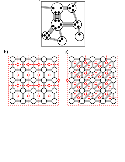
A quantum network is constructed by sharing two-qubit entangled states between locations that we call ‘nodes’. All quantum operations must be local to these nodes but classical communication is allowed between them. The shared two-qubit states are referred to as ‘edges’ and all of the edges between two nodes constitute a ‘bond’ (see Fig. 1). Ideally each edge will be a maximally entangled singlet, however due to decoherence this situation is unrealistic and we must have a method to cope with errors. In this section we will devise a global error correction method that performs local measurements and, by combining the results, information is obtained on the error locations. This information does not allow us to exactly locate the errors but, as we will see, does allow the errors to be subdued so entanglement can be created between distant nodes. Note that throughout we assume the measurements and operations act perfectly.
We will consider the entire network as a mixture of pure states and analyze the protocol acting on each of these using the stabilizer formalism Nielsen and Chuang (2000). From these results we can then determine the mixed state produced. To begin we construct the network’s initial state using the states of individual edges. Each of these initial two-qubit edge states can be transformed into a probabilistic mixture of Bell states Bennett et al. (1996b), via LOCC. This allows us to assume that each edge is in one of the four Bell states given by , where . A stabilizer generated by can then describe each Bell state and we label the probability of that state as . For a network that contains of these identical edges, and qubits, the whole state will have the form
| (1) |
where each edge, , has parameters and . The summations are over all values that these can take and give a mixture of pure states
| (2) |
that occur with probability
| (3) |
The error model we consider has independent bit-flip and phase-flip errors. For this case the pure states that contribute to the mixture can be thought of as networks of error free singlet states, , on which errors randomly occur. A bit-flip error that causes occurs with probability . Similarly, phase-flip errors cause and have a probability of . This situation is equivalent to having edges with the values and and it simplifies the probability of each state to become
| (4) |
with and giving the number of bit-flip and phase-flip errors on the state, respectively,
| (5) |
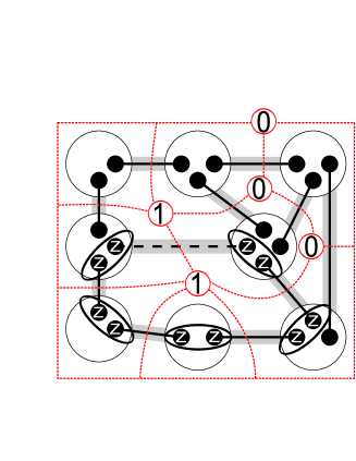
Now we apply the global error correction procedure to one of these pure states. Each of which can be described using a stabilizer that is formed by the union of Bell state stabilizers. The procedure extracts information by performing measurements locally on nodes along a closed path of edges, as illustrated in Fig. 2. Such paths are referred to as ‘loops’ and contain edges from the set , where the give the index of each of the edges forming the loop. These measurements take and as possible values. The product of the measurement results around a loop is labelled . Here gives the bit-flip error parity around the loop, . Each value of gives us information on the errors that we can then use. As the measurements are made the stabilizer follows the rules given in Ref. Nielsen and Chuang (2000). After each measurement the stabilizer generator is manipulated so that at most one element anti-commutes with the measurement operator and the measurement operator, multiplied by the outcome, is then substituted in place of the anti-commuting element. If the operator does not anti-commute with any elements in the stabilizer then nothing is changed.
We obtain the measurement outcomes, (), for the operator between every pairing of qubits in each node. By making these measurements we can calculate for all of the smallest possible loops in the network, which we refer to as plaquettes, and can then deduce for any loop. We do not need to perform the actual measurement between every qubit pair in a node because some of the operators will be products of previously measured operators. From the state these measurements result in a state given by a stabilizer that has generators , ) for every edge, , and operators for every measurement .
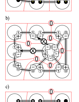
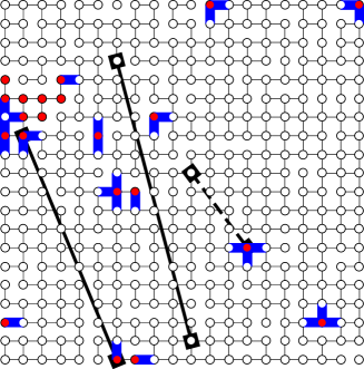
All of the plaquettes in the network can then be assigned their values of . Values of one can be considered as defects on nodes in the dual network (see Fig. 2). These defects occur in pairs. A chain of errors, , on the quantum network’s edges separate the dual node defects in each pair (see Fig.3a). These error affected edges must cross a path of dual network edges that connect the two defects. Hence, we can obtain information on the location of bit-flip errors by pairing the defects, in a matching problem. We assume that the length of the paths is minimal, since longer paths require more errors and this is unlikely when is small. This gives us a minimum weight matching problem to be solved Edmonds (1965) in an analogous way to the correction methods used in surface codes Kitaev (1997, 2003); Dennis et al. (2002). By doing so we have found the most likely defect pairs to be linked by a path of errors. The actual path is assumed to be the one of shortest distance, i.e. smallest number of edges, linking the defects on the dual network (see Fig.3a). Sometimes more than one such path exists and we would wish to minimize the number of nodes between the true path and the assumed path. This can be easily done on regular networks, by using paths that approximately follow straight lines, but for simplicity in the general case it is sufficient to choose one of the shortest paths at random. One qubit in each network edge that lies along the assumed paths is then acted on with a X gate. We can actually avoid performing these X gates until the very end when we may have fewer qubits to apply gates on. Here we include the gates at this stage for clarity. When these gates are applied to a qubit we also change the value of to for each measurement pairing that includes those qubits (see Fig.3b). This gives for an even number of times around every loop and by acting around every loop with gates we can force for every local qubit pairing. A procedure to accomplish this task is given in Fig.3(b-c). Once this is done the resulting stabilizer will have generators , for every edge, , and from every local pairing of qubits. The values have been changed to after performing the gates. These values are unknown, however all of the dual edges that cross edges with must form loops on the dual network. This stabilizer describes a pure GHZ state that has had Z operators acting on it and X operators acting on all the qubits within some nodes. These affected nodes are within loops on the dual network and appear as patches (see Fig. 4). The X gates that remain when the procedure is run on an initial configuration are described by an operator , that applies X gates on the qubits that lie within patches. The whole procedure will result in a mixture of these pure states,
| (6) |
where acts on an arbitrary qubit and is the probability of the initial error configuration being given the results of the measurements.
Larger patches require more errors and are less likely to occur. Hence, for low values of the most probable case is that finite sized patches, containing a small number of nodes, occur randomly. We quantify the probability of a random node existing in a patch as , which has the same value throughout the network. For larger values of the likely number of errors increases so that it becomes impossible to match the defects up correctly and accurately guess the paths. Within infinite networks there exists a critical value of below which patches almost certainly exist and long distance entanglement can be generated. Above the critical value this is not possible and for the most likely pure states.
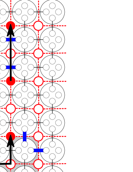
When we are highly likely to form patches the resulting mixed state can be cut back to an impure GHZ state, with any number of qubits up to , by removing qubits with X measurements and, depending on their outcomes, applying a correcting Z operation on one of the qubits to be kept. The final fidelity, i.e. overlap with a pure GHZ state, is dependent on and decreases for more qubits in the resulting state. It is however still independent of the distance between the qubits. In particular, we can remove all of the qubits except two leaving a two-qubit entangled state spread between two nodes. For each pure state contributing to the mixture in Eq. (6) after removing the qubits we obtain an ideal singlet when the remaining qubits are either both in an error affected patch or outside of them (see Fig. 5). The pure state is transformed to the state , that has the form
| (7) |
and the final mixed state is given by the weighted sum of these,
| (8) |
Since is independent of the state separation we see that as long as there are no phase errors present, i.e. , the state produced has a fidelity that is independent of the node separation. These states that do not experience phase errors are called binary states Dür et al. (1999). Our global error correction procedure is a generalization of the one given in Perseguers et al. (2008b) but does not involve teleporting qubits and can be easily applied to any network geometry. Later we will see that we can randomly transform states into binary states, obtaining them on random bonds but also destroying all of the entanglement in the remaining bonds. Our scheme can still be applied in these situations and in Fig. 5 it has been applied on a contributing term in the largest cluster of a square network that was missing such bonds. We will discuss this in more detail in the next section (see Sec. III). Furthermore, in regular networks with all bonds intact we performed simulations to reveal the critical threshold of below which long distance entanglement distribution is always possible. This was done for both square and triangular networks (see Fig. 1(b-c)). In both cases we see the final states fidelity decrease suddenly after critical values (see Fig. 6). These transitions become more prominent for larger networks and later we will attach values to the thresholds.

If we have both bit-flip and phase errors present the initial edges will be rank four Werner states Werner (1989). To apply the procedure in this case we can use error correction codes to subdue the phase-flip errors Shor (1995); Steane (1996); Nielsen and Chuang (2000). All of the qubits are then replaced with encoded qubits and all operations are replaced with their encoded versions. This technique was looked at in Perseguers et al. (2008b) for a square network using a majority voting CSS code. In this case for bonds containing edges the phase error probability on each encoded edge can be suppressed to . To maintain a constant phase error probability on the final state the number of edges in each bond only needs to increase logarithmically with the size of the network. Unfortunately, this operation also increases the chance of a bit flip on the encoded edge to , which means there is a point where the chance of a bit-flip exceeds the network’s critical value, patches are no longer small and the procedure fails. When is small this still enables the error probability to be substantially reduced. For rank two, binary states, the number of edges required in each bond does not need to scale with distance and yet for rank four states there is a logarithmic scaling. In the following we are interested in extending the constant scaling with states that are of rank three.
III Entanglement Distribution with Rank Three States
Using the global error correction procedure we can cause the edge errors in every pure state in an ensemble to condense into patches on a large GHZ state in such a way that a highly entangled two-qubit state can be generated between two distant nodes. This requires the initial network nodes to be linked by sufficiently entangled binary states. However, in the following we will show that such states can be probabilistically generated from a larger class of rank three states using LOCC. This widens the class of states in a 2D network that allow for long distance entanglement distribution.
It is impossible for a rank two, binary state to be created using anything other than states that are rank three or less. We give a short proof of this fact in appendix A. If we have two rank three states that can be probabilistically transformed by LOCC into states of the form
| (9) |
with and , then they can be probabilistically distilled into a binary state
| (10) |
where
| (11) |
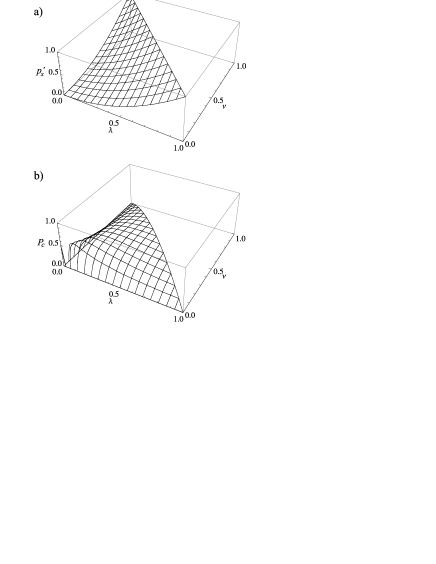
The states given by Eq. (9) can actually form (up to local unitaries) when both qubits of a maximally entangled state, , pass through phase flip and amplitude damping channels. Having two of these states the transformation to a binary state is done by performing a protocol discussed in Ref. Broadfoot et al. (2009, 2010), where it was called a ‘pure state conversion measurement’ (PCM), followed by local Hadamard operations. The PCM involves performing two C-NOT gates locally, with one entangled state’s qubits acting as the target qubits. These target qubits are then measured in the computational basis. If we find both qubits to be in the state it has succeeded, which happens with a probability of . If it fails then we destroy the entanglement and lose both edges used. A graph of and the probability of succeeding is shown in Fig. 7. From this it can be clearly seen that to minimize the resulting we would like to be maximal. The maximal success probability with two states is . If we have initial states in a bond we can generate a binary state with finite probability exceeding , which can be arbitrarily close to one given enough edges. Again, if this fails then all of the edges are lost.
| Lattice | Threshold |
|---|---|
| 2D Square | 0.5 |
| 2D Triangular | |
| 2D Honeycomb |
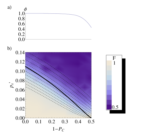
By using this distillation procedure it is possible to transform an initial network composed of rank three states into a network of binary states, where the bonds are missing with a certain probability. This is the case for the network shown in Fig. 5. All of the nodes that are connected by a path of entangled states are then said to be in a cluster. For entanglement to be generated between two nodes they must both be in the same cluster and this links with results from bond percolation theory Bollobás and Riordan (2006). For a square network of infinite extent, if the success probability of transforming each bond into a binary state is larger than then a cluster that contains infinite nodes is almost certain to exist. This is the ‘percolation threshold’ and values for further geometries are given in Tab. 1. The probability of a node being inside the infinite cluster is given by the ‘percolation probability’, . The values of these together with , the probability that a bond exists and is linking nodes in the infinite cluster, can be calculated numerically for different networks Kirkpatrick (1973); Frisch et al. (1962). For large finite networks this threshold phenomenon still exists but the transition becomes smoother. In this case, when the critical value is exceeded we obtain a large cluster that contains a majority of the nodes. On this cluster we can then apply our general global correction procedure to obtain a highly entangled state between two nodes. This requires that the binary states present in the largest cluster are sufficiently entangled for global error correction to succeed. We use entropic arguments to give an approximate threshold for a finite square network, with sides consisting of nodes. The cluster will contain an average of binary states, with each of these introducing a Shannon entropy . The measurements then extract one bit of information from every plaquette in the cluster. The number of these plaquettes on average is given by , with being the average number of nodes in the cluster. We require for enough information to be gathered and this gives a bound for when we solve . These bounds define a region for and within which long distance entanglement distribution can be achieved. In the infinite network case, , we have and can calculate that
| (12) |
This defines the region by the relation and the boundary is shown in Fig. 8. Our procedure is also related to methods developed to cope with qubit loss in surface codes Stace et al. (2009) and similar critical regions have been found in these situations. For the case where the critical value of in an infinite square network is then given by . This can be solved to yield a threshold of . Further analysis for the complete square case is performed in Ref.Perseguers et al. (2008b) and by relating the scheme to surface code error correction Dennis et al. (2002) a threshold of is found. Similarly, in a complete, infinite triangular network we have yielding a threshold of . Both of these thresholds are shown on Fig. 6. In this figure it can be seen that the higher connectivity present in the triangular network does provide for higher fidelity and a lower threshold than a square network. The simulations were run for finite networks so a perfect transition at the critical threshold does not occur. However, as the networks become larger the fidelity will approach for our critical values. Note that these critical values are calculated for the ideal method and will be slightly larger than the simulated threshold due to the random choice of paths.
We have performed numerical simulations of the scheme, when edges are removed randomly, for a 25x25 square network. The final singlet state fidelity for different distillation parameters was calculated and the results are shown in Fig. 8. Our boundary between the values allowing long distance entanglement distribution and those that do not is also shown. This gives a good separation between the parameters producing singlets and those resulting in separable states. There is no sharp transition between the low and high fidelity region which is due to the finite network size. The limiting cases of pure state percolation and binary state global error correction are given by , and , , respectively.
IV Tradeoffs between different strategies on Pure state networks
It is interesting to look at the behavior of entanglement percolation and global error correction when creating long distance entanglement from the same initial network. All of these procedures require a network of identical initial states. If the bonds in the network contain enough entanglement we produce a highly entangled state between two nodes that are a long distance apart. The two nodes that are connected are out of a random set of nodes. Different methods may have benefits such as requiring less entanglement in the initial bonds, generating higher entangled states between two nodes or allowing a greater proportion of nodes to be linked by the entangled state. Pure states are the simplest case where this comparison can be considered so we will look at this case. By randomly generating states between nodes from the initial states and then using global error correction we have found a method that works on networks containing rank three states. By changing the states generated we can apply this scheme on networks of pure states, together with global error correction and entanglement percolation. We will see that there is a wide choice of states to generate and each of these may provide further benefits compared to entanglement percolation or global error correction.
For pure non-maximally entangled states entanglement percolation is known to succeed in creating a long distance singlet state deterministically Acín et al. (2007). This requires a geometry dependent amount of entanglement, related to the percolation thresholds (see Tab. 1). The pure states are characterized by their Schmidt decomposition
| (13) |
with being the largest Schmidt coefficient, . Any pure state can be put into this form via local unitary operations and can be considered as a measure of the state’s entanglement.
Apart from basic entanglement percolation other techniques have also been proposed in pure state networks with smaller initial entanglement requirements Acín et al. (2007); Perseguers et al. (2008a); Lapeyre Jr. et al. (2009); Perseguers et al. (2010). These include the global error correction on a square network with no missing edges, as discussed in Perseguers et al. (2008b), and it was shown that a lower amount of entanglement was required to succeed at the expense of the final states’ fidelity. By randomly generating different states before global error correction it becomes possible to explore the transition between global error correction and entanglement percolation. Here we will again choose to create binary states by probabilistically converting pure states into the binary states. When we start with pure states there are a number of ways to perform this operation. These create the binary states with higher probability of success or more entanglement. To perform the conversion each pure state is transformed, using LOCC, into another pure state
| (14) |
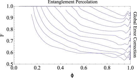
that has higher entanglement with the optimal probability of succeeding . This operation involves a local measurement at one qubit. The result is then communicated to the other qubit where a unitary is performed. This transformation operation and probability come from ‘Majorization’ results Nielsen and Vidal (2001). These states can then be ‘twirled’ Bennett et al. (1996b); Vollbrecht and Werner (2001) into binary states, with . These actions probabilistically generate binary states at random bonds, allowing global error correction to be applied. The value of can be adjusted between and . If is larger than the percolation threshold then an infinite cluster, of binary states , is formed and a node is a member of this cluster with probability . Any two nodes in the cluster can then be linked by global error correction. Two nodes are in the cluster with a probability of and they can be turned into a binary state that has fidelity after global error correction. In Fig. 8 the paths of are shown for different values of as a dashed line. Each point on these lines correspond to a binary state that can be obtained from the initial pure state. The relationship between the available fidelities, , and fraction of nodes in the cluster is given in Fig. 9. Each line relates to a different initial pure state. For each dashed line representing an initial state in Fig. 8 the only points allowing long distance entanglement in the infinite case lie below the critical boundary, shown in Fig. 8.
If we are required to generate long distance entangled states with the highest possible amount of entanglement then, given that the threshold for entanglement percolation is satisfied, the preferred method is to randomly obtain perfect singlets and then use entanglement swapping. This generates a perfect singlet, however in doing so we reduce the number of nodes that are available to be linked. When the threshold is not satisfied we must probabilistically transform the initial states to binary states with the largest that still lie within the critical region. By doing this one highly entangled state is created over a long distance. Note that the initial state of the edges needs to be known in order to decide on the state to percolate. We are unable to choose the nodes before running the protocol, but we still know which nodes are linked at the end. If we are required to link two particular nodes, that have been chosen before the protocol is run, we must maximize and this is achieved by using global error correction. The choice between maximizing the fidelity or is dependent on the intended use for the entangled state. If one entangled state between any two nodes in a set is sufficient it may be beneficial to maximize . In order to judge the schemes a figure of merit can be constructed from and the fidelity. This can then be maximized to reveal the preferred scheme. For example a suitable figure of merit in the case where two specific nodes need to be entangled would be and this is maximized for global error correction.
V Conclusion
Previously, entangled states could only be generated over an arbitrarily long distance from rank two states, or less, in regular 2D networksAcín et al. (2007); Perseguers et al. (2008b); Broadfoot et al. (2009, 2010). Here we have devised a global error correction scheme that enables a highly entangled state to be generated over an arbitrary distance. This procedure can be applied to any network composed of binary states and allows the creation of multi-qubit GHZ states. By combining this with entanglement percolation we have extended this ability to any network and a class of rank three states. These states would result from a combined amplitude damping and phase error channel. For networks composed of these rank three states it becomes possible to produce highly entangled states over arbitrary distances, with constant resources between the nodes. Although this is still a restricted case it is one step closer towards 2D networks composed of full rank states and allows us to deal with two important kinds of noise. Initially there must be a sufficient amount of entanglement between the nodes for the scheme to succeed and we have provided an entropic estimate for the requirements in percolated networks, based on the estimate in Ref. Perseguers et al. (2008b). We have numerically calculated the resulting fidelities and the results agree with the threshold estimate. The behavior of both entanglement percolation and global error correction was previously investigated separately but here we have provided a method to connect these possibilities and in doing so revealed the preferred methods for different priorities. It is still an interesting question to ask whether long distance entanglement distribution can exist in a 2D network of Werner states even when the gates are assumed to be perfect.
This research was supported by the ESF via EuroQUAM (EPSRC grant EP/E041612/1).
Appendix A Impossibility to generate binary states from rank four states
Binary states can not be generated from two-qubit full rank states and we prove this by contradiction. If there were to exist some local procedure that produced some binary states from a full rank state then, by acting after with local projective measurements on all qubits except those in one binary state, we can easily construct a method to generate a single binary state and pure separable state. This local procedure can be described by an operator , where and act locally. The dimension of the entire Hilbert space is . They must also satisfy and . The initial mixed state is
with = 1 and is a complete basis. The procedure can then convert this initial state into
is a pure separable state, is the two-qubit binary state and a non-zero probability. Since the initial state was full rank this property requires to be rank two. This is only the case when either or have rank one. Any operator, , with this property would not generate an entangled state. Hence, a binary state can not be generated using LOCC from a full rank state and this includes the case of finite full rank two-qubit states.
References
- Briegel et al. (1998) H.-J. Briegel, W. Dür, J. I. Cirac, and P. Zoller, Phys. Rev. Lett. 81, 5932 (1998).
- Duan et al. (2001) L.-M. Duan, M. D. Lukin, J. I. Cirac, and P. Zoller, Nature 414, 413 (2001).
- Dür et al. (1999) W. Dür, H.-J. Briegel, J. I. Cirac, and P. Zoller, Phys. Rev. A 59, 169 (1999).
- Hartmann et al. (2007) L. Hartmann, B. Kraus, H.-J. Briegel, and W. Dür, Phys. Rev. A 75, 032310 (2007).
- Dorner et al. (2008) U. Dorner, A. Klein, and D. Jaksch, Quant. Inf. Comp. 8, 0468 (2008).
- Jiang et al. (2009) L. Jiang, J. M. Taylor, K. Nemoto, W. J. Munro, R. Van Meter, and M. D. Lukin, Phys. Rev. A 79, 032325 (2009).
- Bennett and Brassard (1984) C. H. Bennett and G. Brassard, Proceedings of the IEEE International Conference on Computers, Systems, and Signal Processing, Bangalore p. 175 (1984).
- Ekert (1991) A. K. Ekert, Phys. Rev. Lett. 67, 661 (1991).
- Cirac et al. (1999) J. I. Cirac, A. K. Ekert, S. F. Huelga, and C. Macchiavello, Phys. Rev. A 59, 4249 (1999).
- Bennett et al. (1993) C. H. Bennett, G. Brassard, C. Crépeau, R. Jozsa, A. Peres, and W. K. Wootters, Phys. Rev. Lett. 70, 1895 (1993).
- Acín et al. (2007) A. Acín, J. I. Cirac, and M. Lewenstein, Nat. Phys. 3, 256 (2007).
- Perseguers et al. (2008a) S. Perseguers, J. I. Cirac, A. Acín, M. Lewenstein, and J. Wehr, Phys. Rev. A 77, 022308 (2008a).
- Lapeyre Jr. et al. (2009) G. J. Lapeyre Jr., J. Wehr, and M. Lewenstein, Phys. Rev. A 79, 042324 (2009).
- Cuquet and Calsamiglia (2009) M. Cuquet and J. Calsamiglia, Phys. Rev. Lett. 103, 240503 (2009).
- Perseguers et al. (2010) S. Perseguers, D. Cavalcanti, G. J. Lapeyre, M. Lewenstein, and A. Acín, Phys. Rev. A 81, 032327 (2010).
- Kieling and Eisert (2009) K. Kieling and J. Eisert, Quantum and Semi-classical Percolation and Breakdown in Disordered Solids (Springer, Berlin, 2009), vol. 762 of Lecture Notes in Physics, chap. Percolation in quantum computation and communication, pp. 287–319, also available at arxiv [quant-ph] 0712.1836.
- Bennett et al. (1996a) C. H. Bennett, H. J. Bernstein, S. Popescu, and B. Schumacher, Phys. Rev. A 53, 2046 (1996a).
- Bose et al. (1999) S. Bose, V. Vedral, and P. L. Knight, Phys. Rev. A 60, 194 (1999).
- Broadfoot et al. (2009) S. Broadfoot, U. Dorner, and D. Jaksch, EPL (Europhysics Letters) 88, 50002 (2009), URL http://stacks.iop.org/0295-5075/88/i=5/a=50002.
- Broadfoot et al. (2010) S. Broadfoot, U. Dorner, and D. Jaksch, Phys. Rev. A 81, 042316 (2010).
- Perseguers et al. (2008b) S. Perseguers, L. Jiang, N. Schuch, F. Verstraete, M. D. Lukin, J. I. Cirac, and K. G. H. Vollbrecht, Phys. Rev. A 78, 062324 (2008b).
- Perseguers (2010) S. Perseguers, Phys. Rev. A 81, 012310 (2010).
- Nielsen and Chuang (2000) M. A. Nielsen and I. L. Chuang, Quantum Computation and Quantum Information (Cambridge University Press, Cambridge, 2000).
- Bennett et al. (1996b) C. H. Bennett, G. Brassard, S. Popescu, B. Schumacher, J. A. Smolin, and W. K. Wootters, Phys. Rev. Lett. 76, 722 (1996b).
- Edmonds (1965) J. Edmonds, Canadian Journal of Mathematics 17, 449 (1965).
- Kitaev (1997) A. Y. Kitaev, Quantum Communication, Computing, and Measurement pp. 181–188 (1997), hirota, O Holevo, AS Caves, CM 3rd International Conference on Quantum Communication and Measurement SEP 25-30, 1996 SHIZUOKA, JAPAN.
- Kitaev (2003) A. Y. Kitaev, Annals of Physics 303, 2 (2003).
- Dennis et al. (2002) E. Dennis, A. Kitaev, A. Landahl, and J. Preskill, Journal of Mathematical Physics 43, 4452 (2002).
- Werner (1989) R. F. Werner, Phys. Rev. A 40, 4277 (1989).
- Shor (1995) P. W. Shor, Phys. Rev. A 52, R2493 (1995).
- Steane (1996) A. M. Steane, Phys. Rev. Lett. 77, 793 (1996).
- Bollobás and Riordan (2006) B. Bollobás and O. Riordan, Percolation (Cambridge University Press, Cambridge, 2006).
- Lorenz and Ziff (1998) C. D. Lorenz and R. M. Ziff, Phys. Rev. E 57, 230 (1998).
- Kirkpatrick (1973) S. Kirkpatrick, Rev. Mod. Phys. 45, 574 (1973).
- Frisch et al. (1962) H. L. Frisch, J. M. Hammersley, and D. J. A. Welsh, Phys. Rev. 126, 949 (1962).
- Stace et al. (2009) T. M. Stace, S. D. Barrett, and A. C. Doherty, Phys. Rev. Lett. 102, 200501 (2009).
- Nielsen and Vidal (2001) M. Nielsen and G. Vidal, Quant. Inf. Comp. 1, 76 (2001).
- Vollbrecht and Werner (2001) K. G. H. Vollbrecht and R. F. Werner, Phys. Rev. A 64, 062307 (2001).