Spatial clustering of interacting bugs:
Lévy flights versus Gaussian jumps

Abstract

A biological competition model where the individuals of the same species perform a two-dimensional Markovian continuous-time random walk and undergo reproduction and death is studied. The competition is introduced through the assumption that the reproduction rate depends on the crowding in the neighborhood. The spatial dynamics corresponds either to normal diffusion characterized by Gaussian jumps or to superdiffusion characterized by Lévy flights. It is observed that in both cases periodic patterns occur for appropriate parameters of the model, indicating that the general macroscopic collective behavior of the system is more strongly influenced by the competition for the resources than by the type of spatial dynamics. However, some differences arise that are discussed.

1 Introduction

Interacting particle systems help to model and understand various problems in many diverse fields. In biological contexts they are particularly important to study aggregation phenomena of individuals. Fish schools, insect swarms, bacterial patterns, bird flocks and patchy plankton structures are just a few examples revealing the ubiquity and fundamental importance of organism aggregates.

An attempt to address a simple mechanism giving rise to the clustering of particles (with emphasis on plankton patchiness) was made within a Brownian bug model [1] (see also refs. [2, 3]). The model consists of an ensemble of particles (bugs), each one dying or reproducing with a given probability and undergoing Brownian motion. If the diffusivity of the particles is low enough, macroscopic spatial clustering occurs, since a newborn is located close to the parent but particles can die anywhere. If diffusivity is large, particles perform more extended walks and the region that was left empty due to the death of a particle, is occupied fast by some other particle. Similar results were obtained in refs. [4, 5, 6, 7] where lattice-models were studied.

The basic Brownian bug model lacks any interaction between the particles. In a more realistic model (interacting Brownian bug model) the inter-particle interaction was taken into account assuming that the birth and death of individuals depend on the number of other bugs in the neighborhood [8, 9, 10, 11, 12, 13]. For appropriate parameters, a salient property of that model is the formation of spatially periodic clustering of bugs [8]. For large diffusion the clusters become blurred and the periodic pattern is replaced by a more uniform distribution of bugs. Importantly, whereas the positive correlations leading to clustering in the non-interacting bug case arise from the reproductive correlations, i.e., from the fact that offspring is born at the same location of parent [5, 6], the periodic arrangement of clusters in the system of interacting bugs is a consequence of the competitive interaction and has a spatial scale determined by the interaction range $R$ [8].

At the same time it has been observed that many living organisms move consistently with Lévy flight behavior [14, 15, 16, 17, 18]. In particular, the motion of some bacteria is found to be described by Lévy statistics [19, 20], as well as the movement of spider monkeys in search of food [21]. The Lévy type of motion has been shown to be advantageous with respect to standard Brownian motion in some searching strategies involving foraging [18], or in order to enhance encounter rates at low densities [22]. The main reason for this resides in the occurrence of occasional long jumps.

However, the impact of Lévy-type diffusion on the properties of organism aggregates has not received much attention thus far. In the present paper we investigate in the context of a simple interacting bug model, continuous in space, how the occurrence of long jumps in the motion of the individuals influences the collective behavior (c.f. ref. [23]). Similarities and differences between the interacting Brownian and Lévy bug systems will be highlighted.

2 Model and numerical algorithm

We consider a system consisting initially of $N_{0}$ pointlike particles, placed randomly in a two-dimensional $L\times L$ square domain with periodic boundary conditions. After the random time $\tau$, a particle $i$, chosen randomly among all the $N(t)$ bugs in the system at the present time $t$, undergoes one of the two events: it either reproduces or disappears. For the birth and death rates of the $i$-th particle we assume [8],

$$r^{i}_{b} = \mathrm{max}\left(0,r_{b0}-\alpha N_{R}^{i}\right)\,,$$ (1)

$$r^{i}_{d} = \mathrm{max}\left(0,r_{d0}+\beta N_{R}^{i}\right)\,.$$ (2)

Here $N_{R}^{i}$ is the number of particles which are at a distance smaller than $R$ from particle $i$, the parameters $r_{b0}$ and $r_{d0}$ are the zero-density birth and death rates, and the parameters $\alpha$ and $\beta$ determine how $r^{i}_{b}$ and $r^{i}_{d}$ depend on the neighborhood; the function $\mathrm{max}()$ enforces the positivity of the rates. Such a choice for the reproduction and death rates introduces an interaction between the bugs. For the random times $\tau$ an exponential probability density with the complementary cumulative distribution

$$p(\tau)=\exp(-\tau/\tilde{\tau})$$ (3)

and a characteristic time $\langle\tau\rangle=\tilde{\tau}=R_{\mathrm{tot}}^{-1}$ is chosen; $\tilde{\tau}$ is the time-scale parameter and

$$R_{\mathrm{tot}}=\sum_{i=1}^{N}(r^{i}_{b}+r^{i}_{d})$$ (4)

is the total rate of all the $N\equiv N(t)$ particles. In the case of reproduction, the new bug is located at the same position $(x_{i},y_{i})$ as the parent particle $i$. After the demographic event, i.e., after each random time $\tau$, all the particles perform a jump of random length $\ell$ in a random direction characterized by an angle uniformly distributed on $(0,2\pi)$ ($\ell$ and the direction of the jump are different for each particle). The new present time is $t+\tau$ and the process is repeated again, until the final simulation time is reached [13].

In order to simulate the system where the particles undergo normal diffusion, a Gaussian jump-length probability density function is used,

$$\varphi(\ell)=\left(\tilde{\ell}\sqrt{2\pi}\right)^{-1}\exp\left[-\ell^{2}/(2{\tilde{\ell}}^{2})\right]\,,$$ (5)

with variance $\langle\ell^{2}\rangle={\tilde{\ell}}^{2}$; $\tilde{\ell}$ is the space-scale parameter. Since we draw the angle specifying the direction of the jump from the interval $(0,2\pi)$, we can neglect the sign of $\ell$. Note that the random walk defined in this way is not exactly the same as the one in which the walker performs jumps extracted from a two-dimensional Gaussian distribution, but it also leads to normal diffusion and allows a more direct comparison with the Lévy case. The corresponding diffusion coefficient is

$$\kappa=\langle\ell^{2}\rangle/(2\langle\tau\rangle)\,,$$ (6)

which expressed through the space- and time-scale parameters reads, $\kappa={\tilde{\ell}}^{2}/(2\tilde{\tau})$. As we choose to fix the value of $\kappa$, then the space-scale parameter is determined by $\tilde{\ell}=\sqrt{2\kappa\tilde{\tau}}=\sqrt{2\kappa/R_{\mathrm{tot}}}$. Note that because the number of particles is changing in time also the quantity $R_{\mathrm{tot}}$ is changing in time. However, as in this paper we investigate asymptotic statistically steady states, the number of particles weakly fluctuates around a well-defined mean value. Thus, the space-scale parameter $\tilde{\ell}$ is fluctuating in time, but this time dependence is not affecting qualitatively the dynamics of the system.

In order to simulate the system where the particles undergo superdiffusion one can use a symmetric Lévy stable probability density function for the jump size, which behaves asymptotically as [17, 14]

$$\varphi_{\mu}(\ell)\approx{\tilde{\ell}}^{\mu}|\ell|^{-\mu-1}\,,\quad\ell\to\pm\infty\quad(|\ell|\gg\tilde{\ell})\,,$$ (7)

with the Lévy index $0<\mu<2$. For all Lévy stable probability density functions with $\mu<2$ the variance diverges, $\langle\ell^{2}\rangle=\infty$, leading to the occurrence of extremely long jumps, and typical trajectories are self-similar, on all scales showing clusters of shorter jumps intersparsed by long excursions. For $0<a<\mu<2$ fractional moments converge, $\langle|\ell|^{a}\rangle<\infty$. Therefore, for the Lévy index in the range $1<\mu<2$ the value of $\langle|\ell|\rangle$ is finite, whereas for $0<\mu\leq 1$ it diverges. The complementary cumulative distribution corresponding to (7) is

$$P_{\mu}(\ell)\approx{\mu}^{-1}(|\ell|/\tilde{\ell})^{-\mu}\,,\quad\ell\to\pm\infty\,.$$ (8)

As a simple form of complementary cumulative distribution function, which is normalizable and behaves asymptotically as (8), we use

$$P_{\mu}(\ell)=(1+b^{1/\mu}|\ell|/\tilde{\ell})^{-\mu}\,,$$ (9)

where $b=[\Gamma(1-\mu/2)\Gamma(\mu/2)]/\Gamma(\mu)$. As before, we can neglect the sign of $\ell$ since the direction of the jump is assigned by drawing an angle on $(0,2\pi)$. Now the diffusion coefficient (6) is infinite, but one can define a generalized diffusion coefficient in terms of the scales $\tilde{\ell}$ and $\tilde{\tau}$ as [14, 17]

$$\kappa_{\mu}={\tilde{\ell}}^{\mu}/(2\tilde{\tau})\,.$$ (10)

Therefore, in the case of the Lévy flights, when fixing the value of $\kappa_{\mu}$, the space-scale parameter is, $\tilde{\ell}=(2\kappa_{\mu}\tilde{\tau})^{1/\mu}=(2\kappa_{\mu}/R_{\mathrm{tot}})^{1/\mu}$.

The model described can be interpreted in the following way: during a time interval $\tau$ each individual moves on average a distance $\ell$ in some direction but only one of them reproduces or dies. For positive values of $\alpha$ and $\beta$, the more neighbors a particle has within the radius $R$, the smaller is the probability of reproduction and the larger is the probability that the bug does not survive, e.g., due to competition for resources. The periodicity of the simulation domain represents the fact that particles can leave and enter the observation area. In the case of long jumps it represents the situation where there is one particle that leaves the domain and another one that arrives from somewhere, perhaps from far away, and its position is basically random in the domain. In principle, one could also simulate the system so that after the inter-event time $\tau$ a randomly chosen particle undergoes one of the three events: reproduction, death, or jump. However, the results obtained are the same as following the procedure described above; one would just have one more parameter, the jump rate, and different numerical values for the other parameters.

Figure 1: Interacting Brownian bugs (a) versus interacting Lévy bugs (b): spatial configuration of particles in the statistically steady state. The parameters are: $r_{b0}=1$, $r_{d0}=0.1$, $\alpha=0.02$, $\beta=0$, and $R=0.1$ (see also text). In the case of Brownian bugs the diffusion coefficient is $\kappa=10^{-5}$. In the case of Lévy bugs the value of Lévy index is $\mu=1$ and the anomalous diffusion coefficient is $\kappa_{\mu}=56\times 10^{-5}$. The average number of particles in the two systems is approximately the same, $\langle N\rangle=2555$ and $\langle N\rangle=2565$, respectively.

3 Results

In the following we set $\beta=0$ in eq. (2) and $\alpha=0.02$ in eq. (1), i.e., the probability of death is constant and the same for all the particles while the probability for the reproduction depends on how crowded the environment is. Also, we use the values $r_{b0}=1$, $r_{d0}=0.1$, $L=1$, and $R=0.1$ in all the figures presented in the current paper. For $\beta=0$ the critical number of neighbors, $N_{R}^{*}$, for which death and reproduction are equally probable for particle $i$, is determined by

$$N_{R}^{*}=\Delta_{bd}/\alpha\,,$$ (11)

where $\Delta_{bd}=r_{b0}-r_{d0}$. If $N_{R}^{i}<N_{R}^{*}$ it is more probable that particle $i$ reproduces and if $N_{R}^{i}>N_{R}^{*}$ death is more likely. In the following we fix the value of the Lévy index to $\mu=1$. The detailed discussion of the influence of the birth and death rates as well as the Lévy index on the results is outside the scope of the current paper and will be presented elsewhere.

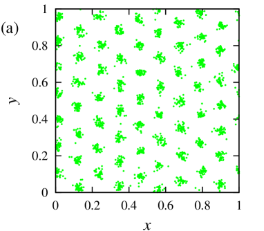
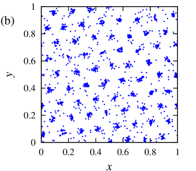
In the case of interacting Brownian bugs, for small enough $\kappa$ and large enough $\Delta_{bd}$, the occurrence of periodic patterns has been observed previously [8, 10]. In the statistically steady state clusters form and arrange in a hexagonal lattice (see fig. 1-a). For large values of the diffusion coefficient the periodic pattern is replaced by an almost homogeneous distribution of particles (see also fig. 3-a). In the case of Lévy flights, since the diffusion coefficient (6) is infinite, one could expect that for the interacting Lévy bugs the spatial distribution will not reveal a periodic pattern. However, as can be seen from fig. 1-b, this is not the case. The reason for the divergence of the diffusion coefficient in the Lévy case is in the statistical weight of the large jumps. These large jumps have some influence in the characteristics of the patterns formed, but the large-scale structure is ruled mainly by the interactions between particles.

For the interacting bug system with Gaussian jumps and moderate diffusion the appearance of periodic clustering is well captured by combining the effects of diffusion and interaction in a mean-field approach [8]. Following the steps in ref. [8] one obtains the following equation as a mean-field approximation to the dynamics of the density of particles $\rho(\textbf{x},t)$ in the interacting Lévy bug model ($\beta=0$):

$$\frac{\partial\rho(\textbf{x},t)}{\partial t}=\rho(\textbf{x},t)\left(\Delta_{bd}-\alpha\int_{D}d\textbf{y}\rho(\textbf{y},t)\right)+\kappa_{\mu}\nabla^{\gamma}\rho(\textbf{x},t)\,\ .$$ (12)

The integration domain $D$ is the set of points within a distance smaller than $R$ from x: $|\textbf{x}-\textbf{y}|<R$. The operator $\nabla^{\gamma}$, with $\gamma=\mu$, is the fractional diffusion operator associated to the Lévy flights of exponent $\mu\in(0,2)$ [14, 17]. It reduces to the standard diffusion operator for $\mu>2$. In this mean-field description the first term accounts for the net growth of the population, the second one takes into account the non-local contribution associated to the saturation due to the interactions within a distance $R$, and the third term describes the spatial diffusion of particles. Equation (12) differs from the mean-field approximation derived in ref. [8] only in the third term where the standard diffusion operator is replaced by the fractional diffusion operator and the diffusion coefficient by the generalized diffusion coefficient. Similar descriptions of reaction-diffusion systems with a fractional diffusion term can be consulted, e.g., in refs. [24, 25, 14, 15].

Figure 2: Comparison of the radial distribution functions for the systems with Gaussian jumps and with Lévy flights. The parameters are as in fig. 1.

Figure 3: Radial distribution function for the system with (a) Gaussian jumps and (b) Lévy jumps for several values of the diffusion and generalized diffusion coefficient, respectively. The other parameters are as in fig. 1 (see also text).

Equation (12) has always the uniform solution

$$\rho(\textbf{x},t)=\rho_{0}=\Delta_{bd}/(\alpha\pi R^{2})\,,$$ (13)

which turns out to become unstable for small $\kappa_{\mu}$ and/or large $\Delta_{bd}$ (what is small or large depends also on the value of $\mu$). This can be seen by introducing the ansatz $\rho(\textbf{x},t)=\rho_{0}+\delta\rho(\textbf{x},t)$ in eq. (12) and linearizing in $\delta\rho(\textbf{x},t)$. The result is

$$\delta\rho(\textbf{x},t)\sim\exp(i\textbf{k}\cdot\textbf{x}+\lambda(\textbf{k})t)\,,$$ (14)

with

$$\lambda(|\textbf{k}|)=-\kappa_{\mu}|\textbf{k}|^{\gamma}-2\Delta_{bd}J_{1}(|\textbf{k}|R)/(|\textbf{k}|R)\,;$$ (15)

$J_{1}$ is a Bessel function. An instability of the uniform solution will occur if the sign of $\lambda(|{\bf k}|)$ changes from negative to positive at some value of $|{\bf k}|$. This will occur first for the critical wavenumber $|{\bf k}_{c}|$ for which $\lambda(|{\bf k}|)$ is maximum. The instability will develop in a periodic pattern which, at least close enough to the instability, will have a periodicity $\delta=2\pi/|{\bf k}_{c}|$. Introducing a dimensionless wavenumber $q\equiv|{\bf k}|R$ and growth rate $\Lambda=R^{\gamma}\lambda/\kappa_{\mu}$, eq. (15) reads,

$$\Lambda(q)=-q^{\gamma}-\nu J_{1}(q)/q\ .$$ (16)

The latter equation shows that, within this mean-field description, the relevant parameters are $\gamma$ (or $\mu$) and the dimensionless quantity $\nu\equiv 2R^{\gamma}\Delta_{ab}/\kappa_{\mu}$. Imposing the condition $\Lambda(q)=0$, corresponding to the change of sign in the growth rate, and $\Lambda^{\prime}(q)=0$, corresponding to the maximum of the growth rate, one can find the critical value of $\nu$, $\nu_{c}=-q_{c}^{\gamma+1}/J_{1}(q_{c})$, and the equation for the critical wavenumber:

$$q_{c}J_{2}(q_{c})/J_{1}(q_{c})=-\gamma\,.$$ (17)

Numerical solution of the latter equation provides $q_{c}$, and therefore $\delta$, as a function of $\gamma$ (or $\mu$), and that $\delta$ is proportional to $R$. In order to make a comparison with the results from numerical simulations of the system, one should keep in mind that the periodic boundary conditions will change $q_{c}$ to the closest number of the form $(2\pi R/L)\sqrt{n^{2}+m^{2}}$ with $n$ and $m$ integers. For $\mu=1$ the value of $\delta$ obtained from the mean-field approximation is $0.128036$ and for $\mu=2$ (Gaussian case) it is $0.131306$, i.e., the periodicity of the pattern is in both cases of the order of $R=0.1$.

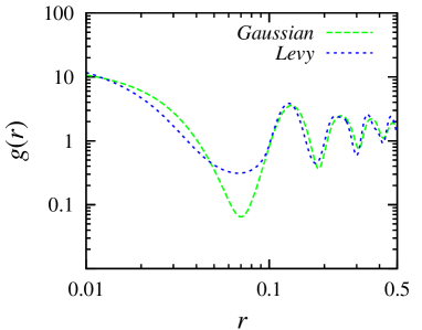
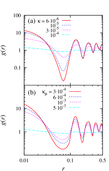
To extract the periodicity of the pattern from the numerical simulations of the system, it is useful to study the radial distribution function $g(r)$. It describes how the density varies with the distance from a given particle respect to the one expected from a uniform distribution, giving thus additional information about the distribution of bugs [26]. It is computed in the standard way, i.e., by counting all particles, $dn$, at a distance between $r$ and $r+dr$ from the target particle, using the formula $dn=(N/L^{2})g(r)2\pi rdr$, and averaging over all particles and different long times. In fig. 2 the comparison of the radial distribution functions for the Brownian and Lévy bugs (for the same systems as in fig. 1) is depicted. Figure 3-a shows the behavior of $g(r)$ in the case of Brownian bugs and in fig. 3-b in the case of Lévy bugs for various values of diffusion coefficient and generalized diffusion coefficient, respectively. The second maximum of $g(r)$, indicating the periodicity of the pattern, appears in fig. 3-a (in the systems of Brownian bugs), up to $\kappa=10^{-5}$, at $0.13125$ and in fig. 3-b (in the Lévy case), up to $\kappa_{\mu}=10^{-3}$, at $0.12875$, being in good agreement with the results obtained from the mean-fieled approximation, and becoming slightly larger only at larger values of $\kappa$ and $\kappa_{\mu}$. The anomalous exponent $\mu$ has only a very light influence on the periodicity of the pattern, which is of the order of $R$ (see also fig. 2 where the slight shift can be can be noticed).

Figure 3 shows also that as $\kappa$ or $\kappa_{\mu}$ increases, the first peak of $g(r)$ gets lower and wider: the total number of particles in the system decreases and the clusters become more spread. For large values of diffusivity ($\kappa$ or $\kappa_{\mu}$), the oscillations of $g(r)$ smooth out, indicating that the periodic pattern becomes replaced by a more homogeneous distribution of bugs.

Figure 4: The distribution of cluster sizes for the interacting Brownian bug and Lévy bug models. All parameters have the same values as in figs. 1 and 2.

Figure 5: Cross-section of the two-dimensional particle density of the average cluster in (a) linear and (b) semi-log scale. Comparison between the interacting Brownian and Lévy bug models. The values of the parameters are the same as in figs. 1, 2, and 4. The continuous lines correspond to the fitting with Gaussian functions.

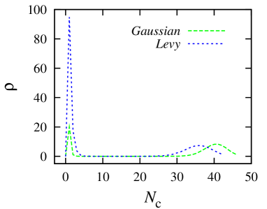
As a difference compared to the case of interacting Brownian bugs, we observe that now, even at small values of $\kappa_{\mu}$, there are many solitary particles appearing for short time periods in the space between the periodically arranged clusters, due to the large jumps, c.f. figs. 1-a and 1-b. This is even better illustrated by fig. 4 where the probability distributions of the cluster sizes for the systems with Gaussian and Lévy jumps are depicted (for the same systems as in fig. 1, i.e., for the given parameters the values of $\kappa$ and $\kappa_{\mu}$ have been chosen such that the average number of the particles in the two systems is approximately equal). The clusters are defined using the nearest neighbor clustering method [27], with a threshold value 0.025 to define neighbors. As one can see, for the system of interacting Brownian bugs the most probable size of large clusters forming the periodic pattern is $41$ particles whereas for interacting Lévy bugs it is $36$ (the critical number of neighbors is in both cases $N_{R}^{*}=45$). A noticeable difference occurs in the proportion of single-particle clusters: the peak of the distribution at the value characterizing isolated particles ($N_{c}=1$) is much higher in the Lévy flight case. Returning to fig. 2, which refers to the same systems as in figs. 1 and 4, it is to be noticed that the minimum between the first and the second peak is much lower for the system of Brownian bugs. This result is consistent with fig. 4: in the system with Lévy flights, the occurrence of many single particles between the clusters forming the periodic pattern produces a higher inter-cluster density is observed.

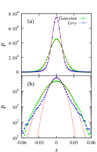
Finally, in fig. 5 the cross-section of the two-dimensional particle density of the average cluster is depicted for the interacting Brownian and Lévy bug systems (same systems as in fig. 1). The average cluster is obtained by setting the origin at the center of mass of each cluster forming the periodic pattern and averaging over all the clusters in the simulation area and over time. In the case of Brownian as well as of Lévy bugs, the central part of the average cluster, where most of the particles are concentrated, is well fitted by a Gaussian function (continuous curve). However, fig. 5-b reveals the difference in the way the particle density decreases in the two systems when moving away from the center of mass of the cluster. Though even in the case of the Brownian bugs the tail of the average cluster is not really well described by a Gaussian function, a Gaussian decay provides a good approximation. Instead, in the case of the Lévy bugs the tail of the average cluster decays slower. Since the average cluster is calculated from individual clusters which are separated by a distance of order $R$, one cannot properly estimate an asymptotic decay, but the decay in the Lévy case seems close to exponential. In any case, it is distinctively faster than the power-law behavior which would be exhibited by clusters of non-interacting particles moving purely by Lévy flights. The existence of the interaction range $R$ introduces a cut-off distance which makes the long-jumps characteristic of Lévy flights not so relevant to determine the large-scale properties of the spatial particle configurations.

4 Conclusion

In the present paper we have studied a simple birth-death model with competition among the individuals of the same species. In particular, we have investigated how the superdiffusive motion of the individuals characterized by Lévy flights influences the collective behavior. We have observed that the appearance of periodic clustering known from previous studies of the interacting Brownian bug model takes place also in the interacting Lévy bug model for appropriate parameters. This is against the expectation that particles performing Lévy flights cannot give rise to space-periodic clustering since their diffusion coefficient is infinite, for which the interacting Brownian bug model is known to reveal no periodic pattern. However, as a difference we have observed that, in the interacting Lévy bug model, due to the long jumps, there are many single particles between the clusters, leading also to the differences in the particle density profiles of the average cluster or in the short-distance behavior of the radial distribution function. From this one can conclude that the large-scale collective behavior of the system is much more strongly influenced by the competitive interaction than by the type of spatial motion performed by the bugs. We have also verified that the mean-field approximation (12) is proper to describe the periodicity in the interacting Lévy bug model.

As a final remark, let us mention that though the model studied in the present article describes rather living organisms, such as animals or bacteria, non-local interactions and Lévy flights are important also in plant ecology for the development of vegetation patterns [28], due to the competition for the resources and because the seed dispersal is often described better by Lévy flights than by Gaussian jumps [29].