A new surrogate data method for nonstationary time series

Abstract

Hypothesis testing based on surrogate data has emerged as a popular way to test the null hypothesis that a signal is a realization of a linear stochastic process. Typically, this is done by generating surrogates which are made to conform to autocorrelation (power spectra) and amplitude distribution of the data (this is not necessary if data are Gaussian). Recently, a new algorithm was proposed, the null hypothesis addressed by this algorithm is that data are a realization of a non stationary linear stochastic process, surrogates generated by this algorithm preserve the autocorrelation and local mean and variance of data. Unfortunately, the assumption of Gaussian amplitude distribution is not always valid. Here we propose a new algorithm; the hypothesis addressed by our algorithm is that data are a realization of a nonlinear static transformation of a non stationary linear stochastic process. Surrogates generated by our algorithm preserve the autocorrelation, amplitude distribution and local mean and variance of data. We present some numerical examples where the previously proposed surrogate data methods fail, but our algorithm is able to discriminate between linear and nonlinear data, whether they are stationary or not. Using our algorithm we also confirm the presence of nonlinearity in the monthly global average temperature and in a small segment of a signal from a Micro Electrode Recording.

1 Introduction

Surrogate data method, initially introduced by Theiler et al. [1] is nowadays one of the most popular tests used in nonlinear time series analysis to investigate the existence of nonlinear dynamics underlying experimental data. The approach is to formulate a null hypothesis for a specific process class and compare the system output to this hypothesis. The surrogate data method can be undertaken in two different ways: Typical realizations are Monte Carlo generated surrogates from a model that provides a good fit to the data; constrained realizations are surrogates generated from the time series to conform to certain properties of the data. The latter approach is preferable for hypothesis testing due to the fact that it does not requiere a pivotal statistics [2]. In order to test a null hypothesis at a level of significance $\alpha$, one has to generate $1/\alpha-1$ ($2/\alpha-1$) surrogates for a one side (two side) test. Then, one simply evokes whatever statistic is of interest and compares the value of this statistic computed from data to the distribution of values elicited from the surrogates. If the statistic value of the data deviates from that of the surrogates, then the null hypothesis may be rejected. Otherwise, it may not.
The classical methods for constrained realizations named (i) Random shuffle (RS); (ii) Random phase (RP); and, (iii) Amplitude adjusted Fourier transform (AAFT) surrogates [1], were developed to test the null hypothesis that the data came from a (i) i.i.d gaussian random process, (ii) linear correlated stochastic process; and (iii) nonlinear static transformation of a linear stochastic process. Surrogates generated with the RS method preserves the amplitude distribution (AD) of the original data, while the ones generated with the RP algorithm preserve the autocorrelation (AC) and surrogates generated with the AAFT algorithm preserve both the AD and the AC of the original data (in general this is not true, this is why an improved version of the AAFT algorithm was presented, referred as iAAFT [3]).
Recently, Richard et al. [4] showed that surrogates generated with the mentioned methods are stationarized versions of the original data. This imply that while the statistical properties of the data might be time dependent, the statistical properties of the surrogates will not. Because of this, when data becomes from a non-stationary process, it is impossible to make a statistical comparison of data with its surrogates. So, the classical surrogate data methods are not applicable to non-stationary process. Due the importance of this kind of process, many modifications of the classical methods have been presented. The first one can be attributed to Schreiber and Schmitz [5], in this approach the surrogate data preserves the AC and any other desired property of the original time series. To generate a surrogate one starts by random shuffling the data, then measuring (for example) the AC of the surrogates and defining an error function as the square difference of data AC minus the surrogate AC. One has to keep permuting pairs until the error function is minimized. To generate surrogates for non stationary time series, one has to ensure that the surrogates also preserve the local mean and variance of the data. This procedure can be done iteratively by means of any optimization algorithm, but there is no guarantee that one will not be stuck in a local minimum (this issue was overcome in [5] by using the simulated annealing optimization method). Unfortunately, this method requires a lot of computational time, so it is of limited applicability.
Recently, Nakamura et al. [6] presented a modification of the RP method which makes it suitable for non-stationary data, they called its method Truncated Fourier Transform (TFT). Surrogates generated with the TFT algorithm are constrained to preserve the AC and the local mean and variance of data so, surrogates will be non-stationary if original data are non-stationary. Through this method it is possible to test the null hypothesis that the data came from a non-stationary linear correlated stochastic process. Since surrogates generated with this method do not preserve the AD of data, further hypothesis (e.g, data are a realization of a nonlinear statical transformation of a non-stationary linear correlated stochastic process) can not be tested. The aim of this paper is to present a new surrogate data method through which is possible to obtain surrogates that are constrained to preserve the AC, AD and local mean and variance of data, but are otherwise random.
This document is organized in the following way; initially we briefly introduce the RP, AAFT and the TFT methods, followed by an introduction to our method, named Amplitude Adjusted Truncated Fourier Transform (AATFT). Then we introduce a methodology to accept or reject a null hypothesis and proceed to apply the methods to several simulated and real time series, showing the utility of each one. Finally we present some concluding remarks.

2 Surrogate data methods

As mentioned, the surrogate data methods, originally introduced by Theiler et al. [1], has become a very popular method for hypothesis testing. The original algorithms can be stated as follows:

2.1 The existing algorithms

2.1.1 Random Phase surrogates (RP)

The surrogate data is generated by the following procedure:

1. Start with the original data $x[t]$, $t=1,\cdots,N$.

2. Compute $z[n]$, the Fourier transform of $x[t]$.

3. Randomize the phases: $z^{\prime}[n]=z[n]e^{\imath\phi[n]}$.
   Where $\phi[1]=0$ and $\phi[n]\in\mathcal{N}(0,2\pi)$, $n=2,\ldots,N$.

4. Symmetrize $z^{\prime}[n]$ (to obtain a real inverse Fourier Transform):
   $z^{\prime}[n-i+1]=\widehat{z}^{\prime}[i+1]$, $i=1,\ldots,floor(n/2)$,
   if $N$ is even then $z^{\prime}[n/2+1]=abs(z^{\prime}[n/2+1])$.
   $\widehat{z}[n]$ is the complex conjugate of $z[n]$.

5. Obtain $x^{\prime}[t]$, the inverse Fourier transform of $z^{\prime}[n]$.

$x^{\prime}[t]$ is the surrogate data of $x[t]$.
The surrogates maintain the linear correlation of the data, but by means of the phases randomization, any nonlinear structure is destroyed.

2.1.2 Amplitude Adjusted Fourier Transform surrogates (AAFT)

The surrogate data is generated by the following procedure:

1. Start with the original data $x[t]$, $t=1,\ldots,N$.

2. Sort the data $Sx[k]$, $k=1,\ldots,N$.

3. Compute $z[n]$, the Fourier transform of $x[t]$.

4. Make a ranked time series $Rx[t]$ defined to satisfy $Sx[Rx[t]]=x[t]$.

5. Create a random data set $g[t]$, $t=1,\ldots,N$.

6. Sort the random gaussian number $Sg[k]$, $k=1,\ldots,N$.

7. Define a new time series $y[t]=Sg[Rx[t]]$.

8. Generate a surrogate time series $y^{\prime}[t]$ from $y[t]$ using the RP algorithm.

9. Make a ranked time series $Ry^{\prime}[t]$ of $y^{\prime}[t]$.

10. The surrogate time series of $x[t]$ is given by $x^{\prime}[t]=Sx[Ry^{\prime}[t]]$.

$x^{\prime}[t]$ is the surrogate data of $x[t]$.
It is evident that this process achieves two aims: First, just as with RP algorithm, the power spectra (and therefore linear correlation) of the data is preserved in the surrogate; and second, the re-ordering process means that the AD of the data and surrogate is also identical (this is actually not true, as this algorithm does not simultaneously preserve both rank distribution and power spectra, which is why the iAAFT [3] has to be used in most practical situations).

2.1.3 Truncated Fourier Transform Surrogates (TFT)

The TFT algorithm introduced a way to deal with non stationarity; this algorithm works by preserving the low frequency phases in the Fourier domain, but randomizing the high frequency components.
The surrogate data is generated by the following procedure:

1. Start with the original data $x[t]$, $t=1,\cdots,N$.

2. Compute $z[n]$, the Fourier transform of $x[t]$.

3. Randomize the phases: $z^{\prime}[n]=z[n]e^{\imath\phi[n]}$. Where
   $\phi[n]\in\mathcal{N}(0,\pi)$ if $n>f_{c}$.
   $\phi[n]=0$ if $n\leq f_{c}$.

4. Symmetrize $z^{\prime}[n]$ (as in the RP algorithm).

5. Obtain $x^{\prime}[t]$, the inverse Fourier transform of $z^{\prime}[n]$.

$x^{\prime}[t]$ is the surrogate data of $x[t]$.
While all phases are not randomized in this method, it is possible to discriminate between linearity and non-linearity because the superposition principle is valid only for linear data. i.e., when data are nonlinear, even if the power spectrum is preserved completely, the inverse Fourier transform data using randomized phases will exhibit a different dynamical behavior.
The surrogate data generated by this method are influenced primarily by the choice of frequency $f_{c}$. If $f_{c}$ is too high, the TFT surrogates are almost identical to the original data. In this case, even if there is nonlinearity in irregular fluctuations, one may fail to detect it. Conversely, if $f_{c}$ is too low, the TFT surrogates are almost the same as the linear surrogate and the long-term trends are not preserved. In this case, even if there is no nonlinearity in irregular fluctuations, one may wrongly judge otherwise. The method for selecting the correct value of $f_{c}$ was presented in [6].

2.2 A new algorithm

2.2.1 Amplitude Adjusted Truncated Fourier Transform surrogates (AATFT)

Surrogates generated with the TFT algorithm do not preserve AD of data (this is actually not true, if $f_{c}$ is high enough the surrogates AD will eventually be like the data AD, but this imply that surrogates are too similar to data). It is tempting to think that this issue can be overcome by simply applying a similar procedure to the AAFT (or the iAAFT) algorithm, but the solution is not so simple. The idea of the TFT method is to preserve the low frequency components of data in surrogates, this is done by preserving some phases of frequency domain, and it is possible to observe that thanks to the reordering procedure of the AAFT method the phases will no longer be preserved.
In order to preserve the AC, AD and local mean and variance of data in surrogates we propose the following procedure.

1. Start with the original data $x[t]$, $t=1,\ldots,N$.

2. Sort the data $Sx[k]$, $k=1,\ldots,N$.

3. Compute $z[n]$, the Fourier transform of $x[t]$.

4. Generate a surrogate time series $x^{\prime}[t]$ of $x[t]$ using the TFT algorithm.

5. Compute $z^{\prime}[n]$, the Fourier transform of $x^{\prime}[t]$.

6. Change the magnitude of $z^{\prime}[n]$:
   $z^{\prime}[n]=\left(z^{\prime}[n]/abs(z^{\prime}[n])\right)abs(z[n])$.

7. Obtain $x^{\prime}[t]$, the inverse Fourier transform of $z^{\prime}[n]$.

8. Make a ranked time series $Rx^{\prime}[t]$ of $x^{\prime}[t]$.

9. Modify $x^{\prime}[t]$ so it has the same data as $Sx[k]$ but with the order given by $Rx^{\prime}[t]$: $x^{\prime}[Rx^{\prime}[t]]=Sx[k]$.

$x^{\prime}[t]$ is the surrogate data of $x[t]$.
If one iteratively performs the steps 5 to 9 it is possible to increase the fitness between AC of the data and the surrogates (the iterative procedure will also reduce the preservation of local mean and variance, but this can be solved increasing the value of $f_{c}$). This iterative procedure will be referred to as iAATFT. Note that surrogate time series $x^{\ {}^{\prime}}[t]$ is just a shuffling of original time series $x[t]$, so it has the same AD.

It is important to notice that any implementation of the discrete FT assumes that the time series under consideration is periodic with a finite period. When there is a large difference between the first and last points (end-point mismatch), the FT will treat this as a sudden discontinuity in the time series. As a result, this will introduce significant spurious high-frequency power into the power spectrum, which is a critical problem when the randomization is centered only on the high-frequency portion.
To ameliorate this artifact, Nakamura et al. [6] proposed to symmetrize the original data before the application of the FT (i.e. $\{x_{1},x_{2},\cdots,x_{n-1},x_{n},x_{n},x_{n-1},\cdots,x_{2},x_{1}\}$). With this procedure, there is no end-point mismatch in the data.

3 Testing for nonlinearity

Next we describe our selection of discriminant statistics, and propose a methodology to accept or reject a null hypothesis using this statistic. Finally we study a method for selecting the correct value of $f_{c}$.
It is important to clarify that we are not interested in performing a deep analysis on the linearity or nonlinearity of any specific time series, our aim is to preset and study the behavior of the new surrogate data method called AATFT; further applications will be presented in the future.

3.1 Selection of the discriminant statistics

Dynamical measures are often used as discriminating statistics. According to [7], the correlation dimension is one of the most popular choices. To estimate these, we first need to reconstruct the underlying attractor. For this purpose, a time-delay embedding reconstruction is usually applied. But this method is not useful for data exhibiting irregular fluctuations and long-term trends, because a smaller time delay is necessary to treat irregular fluctuations and a larger time delay is necessary to treat long-term trends. At the moment, there is no optimal method for embedding such data [7].
Therefore, as discriminant statistics we chose the Average Mutual Information (AMI). The AMI is a nonlinear version of the AC. It can answer the following question: On average, how much does one learn about the future from the past?. For further information regarding the AMI, the reader is referred to [7] and references within.

3.2 Rejection or acceptance of a null hypothesis

Surrogate data methods are based on the Monte Carlo hypothesis testing procedure, first one calculates the statistic for data and surrogates, and then one compares the value of this statistic computed from the data to the distribution of values elicited from the surrogates. If there is sufficient difference the null might be rejected, otherwise it will not.
The level of significance of the test is given by the number of surrogates. For a one sided (two sided) test a level of significance $\alpha$ is reached with $1/\alpha-1$ ($2/\alpha-1$) surrogates.
For robustness, the AMI must be calculated for lag of 1. This calculates on average how much information we have about $\{x_{t+1}\}$ knowing $\{x_{t}\}$. So, if $AMI(\tau=1)$ of the data deviates from that of the surrogates (i.e. is greater or lower) then the null hypothesis may be rejected.
In order to reject (or not) a null hypothesis we generate $N=99$ surrogates, which gaves us a level of significance $\alpha=0.02$.

3.3 Selection of the correct value of $f_{c}$

The selection of the correct value of $f_{c}$ cannot be done a priori, because it depends on the nature of the data and the length of the time series [6]. Our aim is to preserve AC, AD and local mean and variances of the original data in the surrogates. The conservation of AD is assured by the reordering process of the AATFT algorithm. To preserve AC and local mean and variance one has to start by randomizing all the phases ($100\%$ of frequency domain), if AC, local mean and variance of surrogates are not similar to the data then it is necessary to randomize only a portion of the phases (i.e. $99\%$ of the higher frequency domain), and keep decreasing the value of $f_{c}$ by small steps until the surrogates preserve AC, local mean and variance of the original data. It should be noted that it is no possible to preserve the AC for all lags, but at least for small lags the surrogates AC should be identical to the data AC.

4 Results

4.1 Numerical examples

In order to prove the validity of our surrogate data method, we compared results obtained by applying the different algorithms to a fictional time series.

4.1.1 A simple example

First, we analyzed the data generated by a linear AR model given by

$$x(t)=a_{1}x(t-1)+a_{6}x(t-6)+\eta.$$ (1)

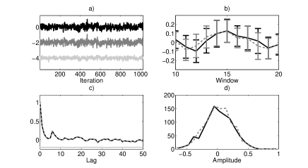
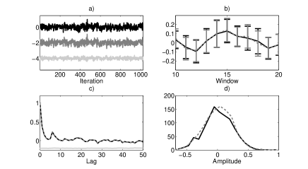
Where $a_{1}=0.3$, $a_{6}=0.2$ and $\eta\in\mathcal{N}(0,1)$. We obtained 2048 values and discarded the first half. Our aim was to prove what has been argued about each algorithm, in this case the acceptance of the null hypothesis is granted. Figs. 1 to 4 show that each algorithm achieves its goals, so using the AATFT algorithm we can generate surrogate constrained to have the same AC, AD and local mean and variance of the data.

Figure 1: a) Original Data (black), surrogate data generated with the RP algorithm (dark gray) and difference between data and surrogate (gray). Values are displaced from one another by 2 for clarity. b) Local Mean and variance of data (black) and surrogates (dotted gray). c) AC of data (black) and surrogates (dotted dark gray), and the difference between AC of data and surrogates (gray). The difference is displaced by 0.2 for clarity. d) AD of data (black) and of surrogates (dotted gray)

Figure 2: a) Original Data (black), surrogate data generated with the iAAFT algorithm (dark gray) and difference between data and surrogate (gray). Values are displaced from one another by 2 for clarity. b) Local Mean and variance of data (black) and surrogates (dotted gray). c) AC of data (black) and surrogates (dotted dark gray), and the difference between AC of data and surrogates (gray). The difference is displaced by 0.2 for clarity. d) AD of data (black) and of surrogates (dotted gray)

Figure 3: a) Original Data (black), surrogate data generated with the TFTS algorithm (dark gray) and difference between data and surrogate (gray). Values are displaced from one another by 2 for clarity. b) Local Mean and variance of data (black) and surrogates (dotted gray). c) AC of data (black) and surrogates (dotted dark gray), and the difference between AC of data and surrogates (gray). The difference is displaced by 0.2 for clarity. d) AD of data (black) and of surrogates (dotted gray). In this case we randomized the higher $98\%$ of the frequency domain.

Figure 4: a) Original Data (black), surrogate data generated with the AATFT algorithm (dark gray) and difference between data and surrogate (gray). Values are displaced from one another by 2 for clarity. b) Local Mean and variance of data (black) and surrogates (dotted gray). c) AC of data (black) and surrogates (dotted dark gray), and the difference between AC of data and surrogates (gray). The difference is displaced by 0.2 for clarity. d) AD of data (black) and of surrogates (dotted gray). In this case we randomized the higher $99\%$ of the frequency domain.

4.1.2 Failure of the iAAFT algorithm

To study the behavior of algorithms in presence of non stationarity we followed [8]. First we defined an AR process.

$$x(t)=a_{1}(t)x(t-1)+a_{2}(t)x(t-2)+a_{3}(t)+\eta.$$ (2)

Where,

$$\begin{split}a_{1}&=2\cos{\left(2\pi/T\right)}\exp{\left(-1/\tau\right)},\\ a_{2}&=-\exp{\left(-2/\tau\right)},\\ a_{3}&=1.\end{split}$$ (3)

This process can be interpreted as a damped oscillator, with period $T$ and relaxation time $\tau$. Period-based modulation is introduced by subjecting the mean period of the AR process to a sinusoidal fluctuation of the form

$$T(t)=T+M_{t}\sin{\left(t2\pi/T_{mod}\right)}.$$ (4)

This modulation introduces a temporal dependency in $a_{1}$:

$$a_{1}(t)=2\cos{\left(2\pi/T(t)\right)}\exp{\left(-1/\tau\right)}.$$ (5)

However, 4 also introduces a temporal dependency in the variance, which can be compensated by using

$$\begin{split}a_{3}(t)^{2}=&\left(\frac{a_{3}^{2}}{1-a_{1}^{2}-a_{2}^{2}-2a_{1}^{2}a_{2}/(1-a_{2})}\right)\\ &\times\left(1-a_{1}(t)^{2}-a_{2}^{2}-\frac{2a_{1}(t)^{2}a_{2}}{1-a_{2}}\right).\end{split}$$ (6)

To generate data, we obtained 2048 values and discarded the first half. Fig. 5 shows the time series (the following parameters were used: $T=50$,$\tau=10$, $T_{mod}=250$ and $M_{T}=5.5$) and a surrogate generated with each algorithm (we excluded the RP algorithm).

Figure 5: Data generated by a linear non stationary AR process (black), surrogate generated by the iAAFT algorithm (dark gray), the TFT algorithm (gray) and the iAATFT algorithm (light gray) each displaced from the other by 2 units for clarity

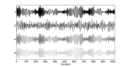
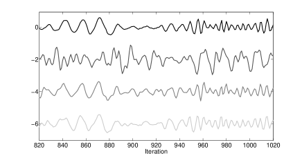
Fig. 6 shows an amplification of Fig. 5, it can be noted that surrogates generated with TFT and iAATFT algorithms preserve the low frequency behavior.

Figure 6: Data generated by a linear non stationary AR process (black), surrogate generated by the iAAFT algorithm (dark gray), the TFT algorithm (gray) and the iAATFT algorithm (light gray) each displaced from the other by 2 units for clarity

Figure 7: AMI ($\tau=1$) for data generated by a linear non stationary AR process (longer stem) and 99 surrogates generad with the a) iAAFT algorithm, b) TFT algorithm and c) iAATFT algorithm (10 iterations were performed). We randomized the higher $99\%$ of the frequency domain.

Finally, Fig. 7 shows the results of computing $AMI(\tau=1)$ for data and $99$ surrogates generated with each algorithm, it can be observed in Fig. 7 a) that the null hypothesis addressed by the iAAFT algorithm was rejected, but this happens because the times series is non stationary not because it is nonlinear. As expected, the hypothesis addressed by TST and AATFT algorithms was not rejected (Timmer [8] proved that the iAAFT algorithm is robust for some kinds of non-stationarity, but as seen here this is not a general result).

4.1.3 Failure of the TFT algorithm

Next we generated surrogates for the following process

$$h(t)=g[x(t)]=x(t)^{2}.$$ (7)

Where $x(t)$ is given by 2. In this case, the signal is nonlinear, but the nonlinearity is given by the observation function $g[\ ]$ rather than by the dynamic of the process.

Figure 8: AMI ($\tau=1$) for data generated by a linear non stationary AR process observed through a nonlinear function (longer stem) and 99 surrogates generad with the a) TFT algorithm and b) iAATFT algorithm (10 iterations were performed). We randomized the higher $98\%$ of the frequency domain.

Fig. 8 shows that the TFT algorithm detects nonlinearity, but the iAAFT algorithm does not. This result was expected, because the hypothesis addressed by the TFT algorithm does not involve a static nonlinear transformation of the linear non stochastic process, while this is exactly the hypothesis addressed by the AATFT algorithm.

4.1.4 Failure of the three methods

We now present a case where neither of the hypotheses are rejected despite the fact that the system that generated the signal is nonlinear. The signal was generated by the Duffing system, given by

$$\ddot{x}+\sigma\dot{x}+\omega_{0}^{2}x+\beta x=\gamma\cos{\omega t}.$$ (8)

In this case, $\sigma=0$, $\omega_{0}^{2}=\gamma=\omega=1$ and $\beta=0.3$. The signal $x$ is obviously nonlinear, but this is a case of weak nonlinearity [9].
Fig. 9 shows 1024 points of the $x$ component of the Duffing equation (integrated for $10.000$ steps with a unit of $0.1$, discarded the first half and then selected a subsegment of $1024$ points which minimized the end-point mismatch) and also shows a surrogate generated with each algorithm. Surrogates generated with each algorithm are very similar to the data, in this case we found that randomizing the higher $95\%$ of the frequency domain, the AC, local mean and variance of data were preserved in the surrogates generated with the TFT and iAATFT methods.

Figure 9: $x$ component of the Duffing equation (black), surrogate generated by the iAAFT algorithm (dark gray), the TFT algorithm (gray) and the iAATFT algorithm (light gray) each displaced from the other by 2 units for clarity

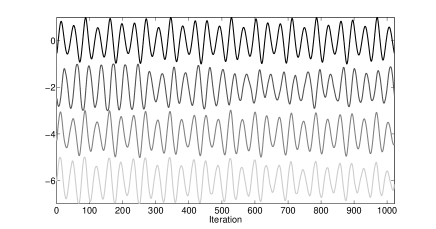
Fig. 10 shows that neither of the hypotheses can be rejected using the AMI. The fact that the test fails to reject the hypothesis could be a consequence of the selected discriminant statistic or just because the nonlinearity is so weak that the test simply fails to detect it.

Figure 10: AMI ($\tau=1$) for $x$ component of the Duffing equation (longer stem) and 99 surrogates generad with the a) TFT algorithm and b) iAATFT algorithm (10 iterations were performed). We randomized the higher $95\%$ of the frequency domain.

4.1.5 A chaotic system

Subsequently, we used the iAAFT, TFT and the iAATFT to generate surrogates for the Lorenz system [7], which is given by

$$\begin{split}\dot{x}&=a(y-x)\\ \dot{y}&=x(b-z)-y\\ \dot{z}&=xy-cz\end{split}$$ (9)

The system exhibits a chaotic behavior with $a=10$, $b=28$ and $c=8/3$.
Fig. 11 shows 1024 points of the $x$ component of the Lorenz system (integrated for $10.000$ steps with a unit of $0.1$, discarded the first half and then selected a subsegment of $1024$ points which minimized the end-point mismatch), and also shows a surrogate generated with each algorithm. It is easy to see that the surrogate generated with the iAAFT algorithm is very different to the data despite it preserve the AC and AD of the data (this situation was also observed in Fig. 5), this imply that data is either: nonlinear and stationary, linear and non stationary or nonlinear and non stationary, but we cannot make a clear distinction.

Figure 11: $x$ component of the Lorenz system (black), surrogate generated by the iAAFT algorithm (dark gray), the TFT algorithm (gray) and the iAATFT algorithm (light gray) each displaced from the other by 2 units for clarity

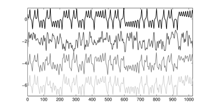
Fig. 12 helps us clarify this issue, it is obvious that data is nonlinear, because the linear and stationary and linear and non stationary hypotheses were rejected.

Figure 12: AMI ($\tau=1$) for $x$ component of the Lorenz system (longer stem) and 99 surrogates generad with the a) TFT algorithm and b) iAATFT algorithm (20 iterations were performed). We randomized the higher $97\%$ of the frequency domain.

4.2 Application to real data

Based on the previous results, we applied the TFT and the AATFT algorithms to two experimental systems: (i) monthly global average temperature (MGAT) from January 1880 to February 2010 (1562 data points). This database is public, available on the web and (ii) Micro electrode recording (MER) from the substantia nigra pars reticulata (4096 data points) adquiared during a Parkinson surgery held in Valencia (Spain). The equipment used in the acquisition was the LEADPOINT TM of Medtronic.

Figure 13: Real time series. a) Monthly global average temperature from January 1880 to February 2010 and b) Micro electrode recording (MER) from the substantia nigra pars reticulata,

4.2.1 Monthly global average temperature (MGAT)

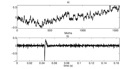
As shown in Fig. 13 a) the MGAT data is non stationary (it has a trend) and has an end point mismatch, so the classical surrogate data methods would not be able to detect nonlinearity. Prior to the generation of surrogate data with the TFT and AATFT algorithms we proceeded to symmetrize the data in order to eliminate the end point mismatch.
Fig. 14 shows that both hypotheses were rejected, so there is a good chance that the data is nonlinear (there is always room for error). This result verifies what was found by [6].

Figure 14: AMI ($\tau=1$) for the Monthly global average temperature from January 1880 to February 2010 (longer stem) and 99 surrogates generad with the a) TFT algorithm and b) iAATFT algorithm (10 iterations were performed). We randomized the higher $98\%$ of the frequency domain.

4.2.2 Micro Electrode recordings (MER)

We now turn our attention to physiological data. Fig. 13 b) shows the typical behavior of these kinds of signals, that is synchronization; the spike is generated because of the synchronization of a small cumulus of neurons sorrounding the micro-electrode implanted in the brain, obviously this is a difficult case and the standard surrogate data methods are useless. However, the TFT and the proposed (AATFT) methods are able to mimic the temporal behavior of data which implies that the preservation of local mean and variance is key to generating valid surrogates. These results are shown in Fig. 15.

Figure 15: MER signal from the substantia nigra pars reticulata(black), surrogate generated by the iAAFT algorithm (dark gray), the TFT algorithm (gray) and the iAATFT algorithm (light gray) each displaced from the other by 2 units for clarity

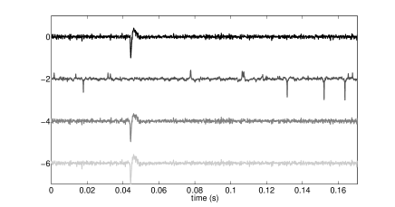
Finally, Fig. 16 shows that the hypothesis addressed by the TFT algorithm is rejected, while the hypothesis addressed by the AAFT algorithm is not. This implies that data is nonlinear, but nonlinearity is due to the observation function, further discussion on this matter will be presented in the future.

Figure 16: AMI ($\tau=1$) for MER signal from the substantia nigra pars reticulata (longer stem) and 99 surrogates generad with the a) TFT algorithm and b) iAATFT algorithm (10 iterations were performed). We randomized the higher $97.5\%$ of the frequency domain.

5 Conclusions

A new surrogate data algorithm was presented. With this algorithm we were able to generate surrogate data that are constrained to the have the same autocorrelation (power spectra), amplitude distribution and local mean and variance of data, but are otherwise realizations of a non-stationary linear stochastic process. In this way we expanded the range of uses for surrogate data methods, by including non stationary and non Gaussian processes. Through numerous examples we demonstrate that classical surrogate data methods will fail to discrimine between linear and nonlinear systems when the underlying process is non-stationary; we also shown that the same problem occurs with the TFT surrogate method when the time series generated by a non-stationary process does not have a Gaussian AD. Only the proposed AATFT algorithm is able to detect the true nature of the data in this cases.
With these methods we were able to confirm the presence of nonlinearity in the monthly global average temperature time series, and we also prove that the studied MER signal is a realization of a nonlinear statical transformation of a linear non-stationary stochastic process, a result that will be studied further in future works.

6 ACKNOWLEDGMENTS

We express our sincere gratitude to the Instrumentation and Control Research Group of the Universidad Tecnológica of Pereira and to the MIRP group in the Research Center of the Instituto Tecnológico Metropolitano of Medellín - Colombia.

References

- Theiler et al. [1992] J. Theiler, S. Eubank, A. Longtin, B. Galdrikian, J. D. Farmer, Testing for nonlinearity in time series: The method of surrogate data, Physica D 58 (1992) 77 – 94.
- Theiler and Prichard [1996] J. Theiler, D. Prichard, Constrained realization monte carlo method for hypothesis testing, Physica D 94 (1996) 221 – 235.
- Schreiber and Schmitz [1996] T. Schreiber, A. Schmitz, Improved surrogate data for nonlinearity tests, Physical Review Letters 77 (1996) 635 – 638.
- Richard et al. [2010] C. Richard, A. Ferrari, H. Amoud, P. Honeine, P. Flandrin, P. Borgnat, Statistical hypothesis testing with time-frequency surrogates to check signal stationarity, in: IEEE Int. Conf. on Acoustics, Speech and Signal Proc. ICASSP 2010.
- Schreiber and Schmitz [2000] T. Schreiber, A. Schmitz, Surrogate time series, Physica D 142 (2000) 346–382.
- Nakamura et al. [2006] T. Nakamura, M. Small, Y. Hirata, Testing for nonlinearity in irregular fluctuations with long-term trends, Physical Review E 74 (2006) 026205.
- Small [2005] M. Small, Applied Nonlinear Time Series Analysis - Applications in Physics, Physiology and Finance, World Scientific, 2005.
- Timmer [1998] J. Timmer, Power of surrogate data testing with respect to nonstationarity, Physical Review E 58 (1998) 5153 – 5156.
- Huang [2005] N. Huang, The Hilbert-Huang Transform in Engineering, Taylor and Francis Group, pp. 1 – 22.