ANITA Collaboration
Ultra-Relativistic Magnetic Monopole Search with the ANITA-II Balloon-borne Radio Interferometer
Abstract
We have conducted a search for extended energy deposition trails left by ultra-relativistic magnetic monopoles interacting in Antarctic ice. The non-observation of any satisfactory candidates in the 31 days of accumulated ANITA-II (Antarctic Impulsive Transient Apparatus) flight data results in an upper limit on the diffuse flux of relativistic monopoles. We obtain a 90% C.L. limit of order for values of Lorentz factor, , at the anticipated energy GeV. This bound is stronger than all previously published experimental limits for this kinematic range.
I Magnetic Monopoles
The search for magnetic monopoles has been the focus of concerted experimental effort since Maxwell’s original formulation of electromagnetism 150 years agoMaxwell65 . The non-observation of an obvious partner to electric charge is somewhat problematic, although inflation provides a mechanism for diluting the primordial monopole abundance to miniscule densities in the current epochGuth81 . Searches have spanned a wide range of monopole masses and Lorentz gamma; all searches assume the Dirac angular momentum quantization condition relating the unit of electric charge to the unit of magnetic charge , via Dirac31 . Thus far, no report of magnetic monopole detectionsPrice75 ; Cabrera82 ; Caplin86 have been substantiatedPrice78 ; Caplin86 ; Huber90 . In 1970, Parker pointed out that the abundance of magnetic monopoles is constrained by the requirement that magnetic monopole currents be insufficient to deplete galactic magnetic fieldsParker70 . Only in the past decade have astrophysical experiments been able to improve upon the original Parker flux bound of Ambrosio02 . The first observational astrophysics experiment to obtain limits stronger than the Parker bound was MACRO. For monopole velocities , MACRO obtained a flux upper limit of . Upper bounds of this order of magnitude were also reported for Ambrosio02 . Subsequently, stronger bounds were reported by the PMT-based neutrino telescopes AMANDAWissing07 and BaikalAynutdinov05 ; Baikalnote , although these latter searches target values of somewhat lower than for the search described herein.
The SLIM experiment at the Chacaltaya High Altitude Laborary in the mountains of Boliva offers sensitivity to so-called Intermediate Mass Monopoles (IMMs). This nuclear track detector experiment is designed especially to search for monopoles (mass GeV) over a wide range of velocities (including for 1-Dirac-charge monopoles). SLIM’s latest monopole flux limit at is for Earth-crossing monopoles, or if upgoing monopoles are absorbed by the EarthBalestra08 . Stronger flux limits based on astrophysical considerations (such as an “extended Parker bound”) of less than for IMMs, using an updated model of galactic magnetic fieldsAdams93 have also been proposed.
Relativistic IMMs
Because of their moderate mass, IMMs may acquire highly relativistic velocities. Wick et al.Wick03 use a model of monopole traversal of intergalactic magnetic fields (similar to the model underlying the Parker bound) to estimate that IMMs created in the early universe would now have typical kinetic energies on the order of GeV. PeV-mass monopoles would therefore reach Lorentz factors . The fact that IMMs acquire such “ultra-relativistic” values provides a mechanism for their detection. Any particle traveling through a medium loses energy, but ultra-relativistic charged particles do so dramatically, initiating bright showersJackson62 . As noted by Wick et al.Wick03 , experiments based on in-ice radiowave detection of showers are particularly well-suited to ultra-relativistic monopole detection because of a combination of large effective volume and favorable scaling with energy. Most recently, the RICE experiment translated their non-detection of radio emissions from compact neutrino-induced in-ice showers into a limit on the relativistic monopole flux using five years of accumulated dataHogan08 . This was not done by a dedicated search, per se, but rather by calculating the efficiency, from Monte Carlo simulations, for monopole-induced showers to pass their neutrino search requirement criteria. It is through detection of such bright showers that ANITA is sensitive to magnetic monopoles.
II ANITA
The Antarctic Impulsive Transient Antenna (ANITA) is a balloon-borne antenna array primarily designed to detect radio wave pulses caused by neutrino collisions with matter, specifically ice. The basic instrument consists of a suite of 40 Seavey Corp. quad-ridged horn antennas, optimized over the frequency range of 200-1200 MHz, with separate outputs for vertically vs. horizontally incident radio frequency signals, mounted on a high-altitude balloon. From an elevation of 38 km, the balloon scans the Antarctic continent in a circumpolar trajectory. After launching from McMurdo Station, ANITA-II was aloft for a period of 31 days with a typical instantaneous duty cycle exceeding 95%.
II.1 Detector Description
Details on the ANITA hardware, as well as the triggering scheme crucial to the analysis described herein, are provided elsewhereANITA_instrumentation_paper . We here provide a brief summary of the hardware elements essential to this analysis.
The front-end Seavey quad-ridge antennas provide the first element in the ANITA radio wave signal processing chain. These horn antennas have separate Vertical (VPol, defined as the zenith direction) vs. Horizontal (HPol) signal polarizations, and each have a field-of-view of approximately full-width-half-maximum (FWHM) in both azimuth angle () and zenith angle (). Two contiguous antennas in azimuth define a logical ‘phi sector’. Following the Seavey antennas, initial signal conditioning restricts the frequency bandpass to that desired for the primary neutrino search, namely, 200–1200 MHz. Signals are then split into a ‘trigger’ path consisting of a heirarchy of trigger conditions (“levels”) and a ‘digitization’ path; if all levels of the trigger are satisfied, the digitized signals are then stored to disk.
II.2 Summary of ANITA missions to date
Hadronic and electromagnetic showers resulting from in-ice neutrino interactions produce a coherent, radio frequency Cherenkov radiation signal. Two one-month long missions (ANITA-1; Dec. 2006-Jan. 2007 and ANITA-II; Dec. 2008-Jan. 2009) have yielded the world’s-best limits to the ultra-high energy (UHE) neutrino flux in the energy range to which ANITA is sensitiveANITA1-jiwoo ; ANITA2-abby . A recent analysis of the ANITA-1 data sample has also provided a statistically large (16 events) sample of self-triggered radio frequency signals attributed to geosynchrotron radiation associated with cosmic-ray induced extensive air showers (EAS)ANITA1-stephen-EAS . The analysis described herein is based on the ANITA-II data sample.
III Monopole Energy Loss in Matter
Essential to this monopole search is a reliable simulation of in-ice showers caused by monopoles traversing the ice sheet. Our model of monopole energy loss is based on the muon/tau energy loss model of Dutta et al.Dutta01 . In this model, energy loss by a muon traversing a medium is expressed as
| (1) |
The term is the energy loss per distance due to ionization of the medium. The termnotebeta is the sum of three terms reflecting bremsstrahlung, pair production, and photonuclear effect energy losses. The values of and of the various contributions to are only weakly dependent.
Although energy loss due to ionization can be treated as smooth and continuous with little loss of accuracy, the stochastic fluctuations in pair production and photonuclear energy losses must be explicitly modeled; such discrete processes, in fact, provide the catastrophic showers to which ANITA-II is most sensitive. The Dutta et al. model expresses these energy losses in terms of partial interaction cross sections with respect to interaction energy, making it possible to isolate the expectation number of particle/medium interactions at a given energy and replace it with a random number of interactions drawn from the appropriate Poisson distribution. To convert the stochastic model of muon energy loss to a model of magnetic monopole energy loss, the muon mass must first be replaced by the magnetic monopole mass. For monopoles, bremsstrahlung is negligible and is disregardedWick03 . Next, due to Dirac’s quantization condition, a magnetic monopole of 1 Dirac charge will lose energy equivalent to an electric charge of times the proton chargeJackson62 . Accounting for this large effective charge only requires multiplying the expectation number of interactions by .
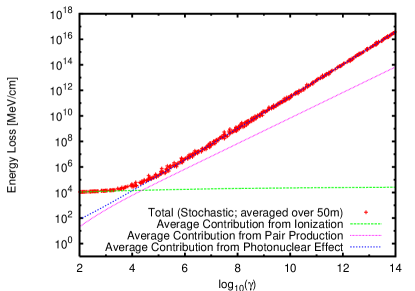
Figure 1 shows various contributions to the energy loss of a GeV monopole. (The monopole rest mass is constrained to vary inversely with gamma such that total energy is fixed at the reference energy of GeV.) The curves indicate average energy loss due to the three principal mechanisms, while the points show actual stochastic energy loss (as averaged over a 50 m interval in our simulation). The photonuclear effect is the dominant energy loss mechanism at , while ionization energy losses dominate below this value. Because the photonuclear mechanism results in hadronic showers generated by nuclear recoils, we may ignore Landau-Migdal-Pomeranchuk (LPM)LPM effects.
IV Monopole Simulation
The monopole energy loss model described above has been incorporated into a Monte Carlo simulation of a magnetic monopole traveling within the ice volume visible to ANITA. The Monte Carlo simulation randomly generates a monopole trajectory (uniform over ) and energy loss according to the previously described model, then determines the voltage response of each of the ANITA antennas which participate in the event trigger, as summarized below and elsewhere. Earth curvature effects, which are considerable at the largest radii (600 km), are incorporated into the model by a suitable adjustment of the refracted ray geometry, relative to the balloon, for a given source location.
IV.1 Passage through Earth
As can be inferred from Figure 1, a down-coming monopole having will easily traverse the entirety of the Antarctic ice sheet without substantial degradation of energy, whereas a normally-incident up-coming monopole at those values will typically range out in the Earth before reaching the South Pole. Upcoming monopoles with larger values will generally reach the detector, although their energy loss in-transit through the Earth can be substantial. For calculating this energy loss, the terrestrial density integrated over the length of the monopole’s path [g/cm2], as a function of approach angle, is taken from the Preliminary Reference Earth ModelDziewonski81 .
IV.2 Propagation Through Ice
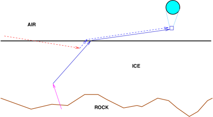
After calculating the energy lost by a monopole en route to the ice target (zero if the monopole arrives from above), the monopole’s interaction with the ice itself is simulated, over discrete step sizes of 15 cm. This selection of step size is motivated by several considerations: a) the time delay between signals received at the ends of the step should be smaller than the time scale of the trigger logic, which is determined by the 7 ns duration of the front-end tunnel-diode signal integration, b) the time delay between successive steps should not be larger than the ANITA digitization time of 0.4 ns, c) the steps should not be so fine that the simulation processing time (and array sizes) become prohibitive. For the most unfavorable geometry (a shower receding from ANITA along the line-of-sight), the time delay between successive steps is the sum of the time for the monopole to move 15 cm in ice plus the additional signal transit time in-air, or approximately 1 ns. However, this geometry results in a Cherenkov pattern undetectable at the payload – similarly, monopoles entering the ice at normal incidence from above () do not illuminate the balloon. Signals typically result when an up-coming monopole transits from rock to ice or a down-coming monopole approaching the balloon is incident on the air-ice interface from above at a near-glancing angle, as illustrated in Figure 2. At the Cherenkov angle of approximately 1 radian, the latter results in zero time delay between successive steps, growing as the azimuthal angle relative to the balloon increases from zero. The former results in a maximum time delay of approximately one time bin between successive steps. The geometric aperture of ANITA to monopoles traversing the ice can be crudely estimated as follows. For a Cherenkov cone developing in the ice, the solid angle illuminating the balloon is approximately the product of the vertical width in (0.2 rads at the lowest frequencies accessible to ANITA) times the horizontal width in (0.5 rads), giving a maximum geometric acceptance of , or approximately 1%. This provides the greatest limitation on ANITA’s sensitivity to monopole signals.
IV.3 Simulated Antenna Response
A Monte Carlo simulation of the radio frequency signals caused by cascades (discussed in Ref.Rice3 ) previously developed in the context of RICE’s high-energy neutrino flux studies has been adapted for application to ANITA. In addition to the stochastic energy loss processes enumerated previously, we also simulate ray-tracing through the firn, as well as signal loss in transmission across the snow surface into the air, as a function of incident angle on the ice-air interface.
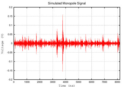
A typical example of a simulated monopole time-domain voltage profile, for a monopole simulated at , is shown in Figure 3. In contrast to temporally compact showers from neutrinos, monopoles deposit energy over a timescale considerably longer than the minimum 400 ns time required to fill four available data acquisition event buffers. Schematically, the monopole signal can be treated as a sequence of ‘subshowers’, each having a characteristic energy deposition geometry and time delay relative to ANITA. As demonstrated by laboratory measurementsslac-testbeam ; slac-salt04 , the frequency-domain radio wave signal due to a shower in a dense medium is typically broad and, in contrast to typical narrow-band anthropogenic backgrounds, extends over hundreds of MHz. The complete simulated voltage profile at each antenna is determined by coherently summing the voltage contributions of various subshowers in each time bin. The signal phase at the emission point will vary slowly with viewing anglebuniy ; however, in most cases the dominant emission arises from a coherent region along the track centered around the Cherenkov point and subtending a small viewing angle. Accordingly, we ignore all signal phases other than those from travel time in our analysis.
Similar to showers from neutrinos, the signal strength is typically at least an order of magnitude stronger along the vertical polarization (VPol) axis compared to the horizontal polarization axis, given the excellent cross-polarization isolation (20 dB) of the Seavey antennas.
IV.4 Trigger Simulation
The heirarchical ANITA-II trigger allows a relatively low neutrino detection trigger threshold, while maintaining a tolerable (Hz) thermal noise data rate written to disk. In contrast to ANITA-I, only signals from the VPol channel of the dual-polarization horn antennas contribute to the ANITA-II trigger. Following the antenna, signals routed through the ‘trigger’ (vs. ‘digitization’) path are tested for their spectral power in four frequency bands, approximately covering the intervals (in MHz) 200350, 330600, 6301100 and 1501240, respectively. This partitioning is performed in order to provide rejection power against narrow-bandwidth anthropogenic backgrounds, while retaining high efficiency for sharp duration (temporally), large-bandwidth neutrino signals. The frequency-banded signals are then passed through a tunnel-diode, which integrates roughly 7-ns units of data and provides a unipolar (negative) output pulse. The lowest-level trigger (L0) requires signal in one of the four frequency bands at a level exceeding approximately 2.3, with the rms of the typical tunnel-diode output voltage at this point. The L1 trigger required two of the three frequency bands plus a full-band trigger within a 10 ns window. (In an improvement over ANITA-1, the different group delays of the bandpass filters from the single-band stage were compensated digitally to ensure synchronization.) The L1 triggers were then combined for the L2 trigger stage. For the upper and lower antennas, an L2 was issued in one of the 16 phi sectors when two of the three antennas either on or adjacent to that phi sector triggered within approximately 10 ns of each other. For phi sectors containing a nadir antenna, an L2 was issued for each L1, and for those without, an L2 was issued when either adjacent nadir antenna received an L1. Finally, the fourth (L3) stage required two of the three antenna rings (upper, lower, and nadir) to have an L2 trigger within approximately 10 ns. Satisfaction of all trigger tiers initiates digitization of all antenna channels and occurs at a rate of approximately 10 Hz. By contrast, the L1 and L2 rates are approximately 2–3 MHz, and 2.5 kHz per antenna pair, respectively. Laboratory studies have demonstrated that trigger efficiency differences between ANITA-1 and ANITA-II result primarily from the removal of the HPol antenna channels from the trigger logic, and the modified frequency banding.
V ANITA Experimental Monopole Detection Strategy
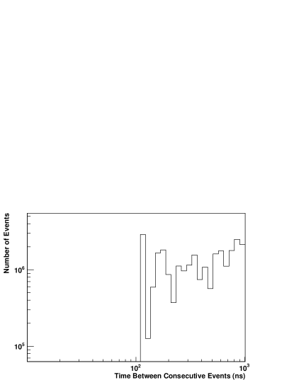
As a monopole interacts with the ice, it sheds energy stochastically, so the monopole signal will be comprised of a string of impulsive subshower events. When ANITA triggers, the signal is temporarily stored in one of four buffers and is then read to hard disk. As soon as one buffer is filled, it is read out and then reset for the next event. Since this process requires some minimum time, if a series of triggers occur in rapid succession (e.g., within 1 s), there is insufficient time to maintain at least one free buffer. Once all four buffers fill, read, clear, and reset commands are sequentially issued, requiring a minimum time of tens of milliseconds, much longer than the monopole signal would be visible to the balloon. The experimental monopole signature registered in ANITA is therefore expected to consist of the first four threshold-crossings (500 nanoseconds total) once the monopole comes into view; the remaining signal produced by the monopole ionization trail is not registered during the dead-time required after the four buffers initially fill. The 500 nanosecond estimate also includes a small delay between successive triggers, as they fill the available buffers. The experimental in-flight data show a minimum time between triggers =112 ns (Fig. 4), to be compared with the 100 ns of data recorded in a standard waveform capture. This value is commensurate with laboratory measurements prior to the flight.
VI Monopole Selection and Event Yield
Our monopole event selection criterion therefore consists of four ‘fast’ triggers over a time interval ; it remains only to define how quickly the triggers must be registered () in order to be considered a monopole candidate. To minimize bias, was determined using a ‘dedicated background’ (DB) subset of the total ANITA dataset, defined as all data taken when the balloon was within 300km of McMurdo base. This subset comprised approximately 15% of the total data. For this dataset, Figure 5 shows the distribution, with the monopole MC simulated distribution overlaid, as well as a polynomial fit to the DB distribution.
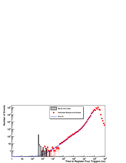
For large values of , the stochastic nature of the monopole energy loss tends to induce threshold crossings at a rate much faster than that at which the instrument can trigger. Since the filling of all buffers will immediately incur tens of milliseconds of subsequent dead time, the simulated distributions therefore exhibit pile-up at the minimum possible value of 3.
From the DB sample, we set the requirement that 500 ns), which eliminates all the background event triggers. This is the main monopole selection criteria then applied to our ‘search’ sample.
VI.1 Trigger Efficiency
Monte Carlo simulations of monopoles isotropically illuminating the Antarctic ice sheet are used to determine the 500 ns efficiency. Although the bulk of high-energy monopoles which produce four triggers also satisfy the 500 ns criterion, the limited geometric acceptance for producing four triggers (1%, designated as “”) provides the main limitation on the total efficiency (designated as “”). The ratio of events satisfying both the simulated trigger (which includes aperture), as well as the 500 ns requirement relative to the total events generated in simulation for each value (typically 20,000), are as follows:
| 8 | 9 | 10 | 11 | 12 | 13 | |
|---|---|---|---|---|---|---|
| () | 0 | 0.43 | 3.85 | 4.35 | 7.19 | 7.69 |
| () | 0 | .06 | 1.65 | 3.17 | 4.66 | 6.12 |
| () | 0 | .04 | .34 | .48 | .99 | 1.20 |
Also shown in the last row are the errors on the total efficiency; our eventual limits will later be degraded by one statistical error bar in each energy bin.
VI.2 Background estimate in search sample
After establishing the requirement that 500 ns based on the DB sample, the trigger time distribution of the remainder of the data set (the monopole ‘search’ sample) was considered. It is desirable that the number of events passing this requirement in the search sample be small enough that they can be individually hand-scanned and their candidacy assessed against Monte Carlo simulated monopole templates. Extrapolating the DB distribution into the ‘signal’ region below 500 ns (Fig. 5) indicates a projected yield of 0.46 events; correcting this by the ratio of livetime in the search sample relative to the DB samples (0.85/.15) results in an a priori expectation of 2.6 background events in the search sample.
Thermal triggers, overall, dominate the accumulated ANITA-II data sample and are responsible for the ‘hump’ to the right in Figure 5. Given the typical L3 trigger rate of 10 Hz, the probability of registering 4 uncorrelated thermal triggers within 500 ns can be estimated to be per second, implying a negligible expected thermal event fake yield in our search sample.
VI.3 distributions in search sample
The distribution for the entire ANITA-II flight is shown in Figure 6.
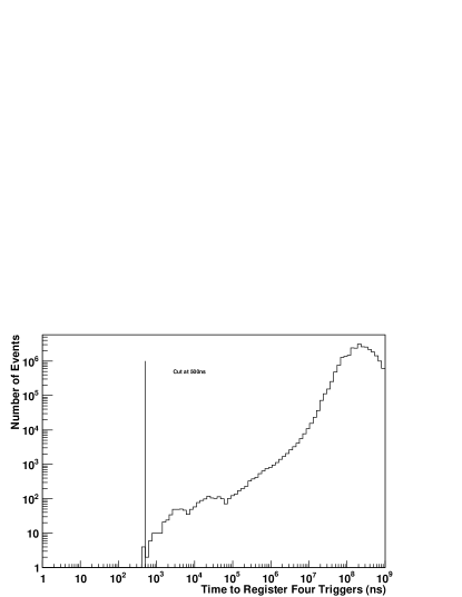
We do note dissimilarities, at small values of , in the shapes of the DB vs. search sample distributions. This is, however, not necessarily surprising, since our DB sample is restricted to data taken in the vicinity of McMurdo Station, while the search sample includes data taken over the entire continent.
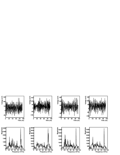
In the entire data sample, only four events contain four rapid triggers which satisfy the 500 ns maximum total trigger time criterion. All four of these events were already classified as background, using the rejection criteria developed for the primary ANITA-II neutrino searchANITA2-abby . Specifically, the first two events were rejected on the basis of their temporal near-coincidence (occurring within 15 seconds of each other) as well as having source locations (after filtering for strong continuous wave [CW] components) consistent, to within 1 degree, with the South Pole. The third event was recognized as payload noise, on the basis of an anomalous DC offset, and saturated waveforms in all phi sectors. The final event was rejected on the basis of its power spectrum, which is observed to be dominated by one narrow CW frequency without which the event would be sub-threshold for analysis. Removing that one line from the frequency spectrum results in a time-domain waveform which also reconstructs to a known background source location in West Antarctica and further affirms this as a background event. The time-domain, as well as frequency-domain distributions for the four highest-amplitude channels in that last event are displayed in Figure 7.
We note similarity in character between that event from the search sample and a typical event with 500 ns from the DB sample (Figure 8).
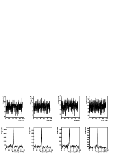
In fact, the power spectra of all the events with 500 ns, in both the DB as well as search samples, are found (a posteriori) to be dominated by CW lines. This is in marked contrast to monopole signals, which exhibit the broadband characteristics of temporally-sharp, coherent radio wavelength signals.
Elimination of these four events in the search sample (roughly consistent with our a priori expectation of 2.6 background events from the DB sample) results in zero candidate monopole triggers in the ANITA-II data set. Since no satisfactory event candidates are found, we therefore choose to set a limit on the monopole flux. However, having invoked criteria (base rejection) used for the primary neutrino search, we also must later degrade our monopole detection efficiency by the geometric loss due to that anthropogenic background requirement ().
VII Cross-check analysis
A complete, and parallel analysis, which was intended to avoid the a posteriori hand scan, was performed as follows. Given the fact that anthropogenic noise tends to be a) CW (continuous wave) in the frequency domain, and b) persisting for durations of order seconds, we initially restrict our candidate search sample to those events satisfying an extended CW-rejection requirement. Starting with the first event of a set of four filled in rapid succession, we transform to the frequency domain and determine the frequency bin with the highest fractional power. For a uniform population, and based on 256 time-domain samples, this quantity would be 1/(256/2), or 1/128. Assuming that, for man-made backgrounds, that bin will also have the highest spectral power for the next 3 events in a candidate quartet, we now calculate the product of the fractional power (“PFP”), for that same bin determined from the first captured event, for all four events in a quartet. For thermal noise, this quantity peaks at around , for Monte Carlo simulations, this distribution peaks at around , primarily because of the fact that: i) monopole candidates are generally close to the thermal floor, and ii) the ANITA trigger requires power in multiple trigger bands. Based on the Monte Carlo distribution, we set a cut on this statistic at , which corresponds to approximately 95% efficiency and high background rejection of the DB sample (Figure 9).

Having set the cut based on Monte Carlo simulations only, we now apply this requirement to the signal search sample; none of the 500 ns data events survives this requirement, resulting (again) in zero monopole candidates. Note that application of this CW-rejection would actually result in a stronger limit than what we finally quote below as we do not incur a penalty of in our efficiency.
VIII Live Time
In order to calculate a flux limit, the time ANITA is sensitive to monopoles must be known. Recall that ANITA must be both active and have four free buffers available to record our “cluster” of events. The buffer depth (“BD”, or the number of available buffers to fill with data triggers) was not always known during flight, so a simulation was developed to estimate the fractional live time contributed by each buffer state. We know that when an event is triggered, a buffer becomes occupied, and the buffer depth decrements (we use the notation “BD=4” to indicate that all buffers are empty; “BD=0” implies all buffers are occupied and dead time is incurred). When an event is read to disk, a buffer is freed and BD increments. Figure 10 is a graphical representation of event acquisition and readout.

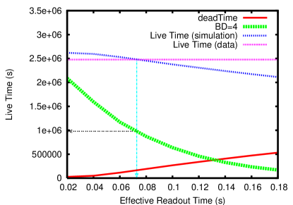
Our simulation provides an estimate of the amount of time spent in each buffer state , where i indicates the buffer depth; the monopole livetime therefore corresponds to . The only variable in the model is the unknown effective readout time , which is determined as follows. The simulation reads through the entire list of trigger times recorded in data. When an event is triggered, our model increments BD and, after has elapsed, BD decrements. If, in the simulation, a trigger occurs when BD=0, the event is simply skipped and BD is left unchanged. Given the typical ANITA-II data trigger rate of 10 Hz, any gaps in triggers greater than 1 second are considered dead time, and following one of these gaps, BD is reset to 0. Despite the individual buffer depth states not being known, the total time ANITA was live () is reliably tracked during flight and provides a constraint on our model. The ‘correct’ is defined as that value for which the simulated converged on the actual .
Figure 11 shows the simulation results as the trial value of is varied from 0.02s to 0.14s. The horizontal magenta line represents the known ; the intersection of this line with the cyan arrow (simulated ) corresponds to the case where the live time constraint is satisfied. Simulation matches data when 73 ms. From this value, our aggregate livetime for BD=4 is estimated to be s.
IX Systematic Errors
The primary source of uncertainty is likely due to the systematic error inherent in our efficiency estimate, primarily due to ice properties uncertainties and our finite time binning procedure (which determines the coherence of the time domain waveform) in simulations. This is assessed by running our simulation with two considerably different sets of parameters. In the first set of trials, the monopole is tracked over a step size of 80 cm, beginning at the first point within the ice sheet when the monopole registers a trigger, and extending for 8192 simulated samples. For high-energy, upcoming monopoles which are capable of arriving from below after traversing the Earth, the monopole is therefore tracked over the warmest, and most birefringent 1.5 km of ice starting at the bottom of the ice sheet. In the second set of trials (our default parameters), the monopole is tracked over a 15 cm step size only over the top (colder ice, with no birefringence) 1.5 km of ice thickness, extending over 16384 simulated samples. The ‘test’ parameters result in approximately 23% lower efficiency than our default parameters, largely due to the generally-smaller measured signal strengths emanating from the deeper, warmer (and significantly more radio-absorbing) ice. This extreme variation should bracket the expected uncertainties due to our radio frequencies ice properties’ parameterization, as well as our finite time-binning procedure for signal, in the limit where the step size is correctly taken to zero.
There is some uncertainty associated with the calculation of the monopole energy loss. To assess this, we have compared our simulation with the monopole energy loss calculated independently by the mmc codedima , which was originally designed for muons and subsequently adapted to model monopoles for the IceCube collaboration. Unlike our simulation, the mmc energy loss parametrization is based on several different theoretical calculations, and also calculates energy losses independently of our simulations. Since the kinematic regime targeted by the IceCube analysis is approximately 5-10 orders of magnitude lower than for this analysis, the overlap between the simulations is limited to gamma values of order . For , we find agreement between the results of the two simulations to within 13.5%.
Our overall result is relatively insensitive to the parametrization of thermal noise in our simulation. The addition of such noise is included in our simulation and will, on average, lead to a noticeable efficiency improvement for very large simulation samples. For our limited simulation samples, however, this effect is mitigated by the stochastic nature of the monopole energy deposition, which leads to a large number of in-ice showers with widely varying energies, and distributed over viewing angles varying by up to several degrees relative to the balloon.
To account for our limited Monte Carlo statistics, we have included an error equal to the fractional statistical precision on our Monte Carlo-derived detection efficiency. To account for the uncertainty in our choice of 500 ns as the optimal monopole event selection requirement, we have also folded in a systematic error equal to the inefficiency of our 500 ns event selection requirement (10%). Added in quadrature with both the energy loss uncertainty (13.5%), as well as the 23% systematic error determined above yields a net systematic error of 28%. Our final upper limit is accordingly degraded by this fraction. Uncertainties in our livetime calculation are believed to be smaller than 5% and can therefore be neglected in our total systematic error. We note that the two dominant systematic errors above are independent of each other – the energy loss uncertainty is assessed without fully propagating the signal to the balloon, while the latter uncertainty measures the error in our modeling subsequent to energy deposition. Note that the final result is somewhat robust to changes in the overall scale of – increasing leads to brighter in-ice showers, but reduces the flux of monopoles that can penetrate to the ice sheet from below the horizon. Conversely, reducing increases the flux arriving at the ice sheet, but decreases the magnitude of signal strength on a monopole-by-monopole basis. In general, ANITA’s sensitivity to relativistic monopoles is primarily determined by the detector/ice geometry. For monopole trajectories that do illuminate the balloon, we expect there to be tens, if not hundreds of potential showers which can cause event triggers. In practice, only the first four of these are recorded by the data acquisition system.
Overall, we have tried to take a conservative approach in calculating our sensitivity, including: a) tracking the monopole over the only the upper half of the ice sheet and neglecting any signal from the lower half which results in a conservative estimate of effective area, b) calculating sensitivity under the assumption that systematic errors are uncorrelated, and therefore forfeiting any numerical advantage that would be gained by taking such correlations into account, c) using an estimated trigger efficiency which is approximately 25% less efficient than that employed for the primary neutrino search.
X Particle Flux Limit Calculation
Particle flux is reported in units of . To calculate an upper bound on the diffuse monopole flux, the upper limit on the number of observed particles (), live time (), detection area (), and the solid angle from which incident particles are approaching () must be known. In this experiment, none of the candidate events met the acceptance criteria, so the number of observed particles is zero, corresponding to a Poisson 90% confidence level upper limit on the number of observed particles of 2.3 (we neglect possible background contributions which, if included, would tend to strengthen our derived upper limit). The BD=4 live time given by the simulation is =975,000 s. The detection area is the surface area of a spherical cap of radius R=680 km and is therefore slightly greater than the planar projection area of (by approximately 5%). Finally, we must include the efficiency for events to both trigger, as well as to pass our 500 ns () requirement, and also the efficiency for events to pass our base rejection requirements () in the expression for particle flux (Eqn. 2); we take to be the value used for the neutrino-search analysis (63%), as those search criteria are invoked during the final phase of the analysis in our elimination of the four events passing the 500 ns requirement from monopole candidacy.
| (2) |
Our final results are shown in Figure 12. We obtain a flux limit of order at , improving slowly over the next few decades in monopole . For large gamma values, the results for ANITA are considerably lower than that of any experiment to date.
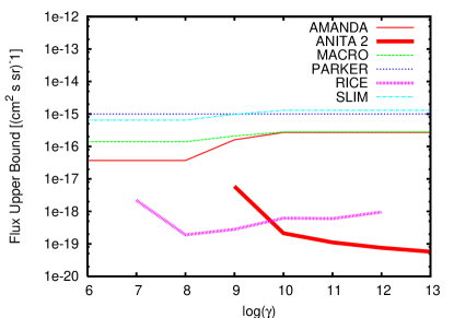
Although the bandpasses of the RICE and ANITA experiments are comparable, the ANITA analysis strategy is directed at monopole detection , affording a factor of three improvement in efficiency relative to the RICE analysis, which was driven by a neutrino search strategy. The additional enhancement in effective collection area (500, including losses in collection area due to rejecting bases) more than compensates ANITA’s factor of 50 smaller livetime relative to RICE.
XI Summary
From the non-observation of highly ionizing showers we have derived the monopole flux upper limits shown in Fig. 12, which are on the order of . Previously, AMANDAWissing07 , BaikalAynutdinov05 , and MACROAmbrosio02 determined monopole flux limits on the order of for greater than , , and , respectively. Although the results of this study cover a much narrower range of values than previous works, it is the range that is of the greatest interest for IMM searches. Within much of this kinematic range ( GeV; ), monopole flux limits from ANITA are stronger than the limits from any previous astrophysical monopole search.
Acknowledgments We thank the National Aeronautics and Space Administration, the National Science Foundation Office of Polar Programs, the Department of Energy Office of Science HEP Division, the UK Science and Technology Facilities Council, the National Science Council in Taiwan ROC, and especially the staff of the Columbia Scientific Balloon Facility.
References
- (1) Maxwell, James Clerk, “A Dynamical Theory of the Electromagnetic Field”, Philosophical Transactions of the Royal Society of London 155, 459-512 (1865).
- (2) A.H. Guth, Phys. Rev. D23, 347 (1981).
- (3) P.A.M. Dirac, Proc. Roy. Soc. London A133, 60 (1931).
- (4) P.B. Price, E.K. Shirk, W.Z. Osborne, and L.S. Pinsky, Phys. Rev. Lett. 35, 487 (1975).
- (5) B. Cabrera, Phys. Rev. Lett. 48, 1378 (1982).
- (6) A.D. Caplin, M. Hardiman, M. Koratzinos, and J.C. Schouten, Nature 321, 402 (1986).
- (7) P.B. Price, E.K. Shirk, W.Z. Osborne, and L.S. Pinsky, Phys. Rev. D18, 1382 (1978).
- (8) M.E. Huber, B. Cabrera, M.A. Taber, and R.D. Gardner, Phys. Rev. Lett. 64, 835 (1990).
- (9) E.N. Parker, Astrophys. J. 160, 383 (1970).
- (10) M. Ambrosio et al. (MACRO Collaboration), Eur. Phys. J. C25, 511 (2002).
- (11) H. Wissing, for the IceCube Collaboration, in Proceedings of the 30 International Cosmic Ray Conference (ICRC), Merida, Mexico, 2007.
- (12) V. Aynutdinov et al. (Baikal Collaboration), in Proceedings of the 29 International Cosmic Ray Conference (ICRC), Pune, India, 2005.
- (13) The flux limit from Baikal assumes an initial monopole energy of GeV, lower than the initial energy assumed in this study. Therefore, the Baikal limit shown in Fig. 12 should be regarded as a function of the indicated mass but not necessarily the indicated .
- (14) S. Balestra et al. (SLIM Collaboration), Eur. Phys. J. C55, 57 (2008).
- (15) F.C. Adams, M. Fatuzzo, K. Freese, G. Tarlé, R. Watkins, and M.S. Turner, Phys. Rev. Lett. 70, 2511 (1993); astrophysical limits tabulated in Eidelman04
- (16) S.D. Wick, T.W. Kephart, T.J. Weiler, and P.L. Biermann, Astropart. Phys. 18, 663 (2003).
- (17) J.D. Jackson, Classical Electrodynamics (Wiley, New York, 1962).
- (18) P. W. Gorham et al. (ANITA Collaboration), Astropart. Phys. 32, 10 (2009).
- (19) D.P. Hogan et al., Phys. Rev. D78, 075031 (2008).
- (20) A. Vilenkin and E.P.S. Shellard, Cosmic Strings and Other Topological Defects (Cambridge University, Cambridge, 1994).
- (21) K. Greisen, Phys. Rev. Lett. 16, 748 (1966); G. Zatsepin and V. Kuzmin, Pis’ma Zh. Eksp. Teor. Fiz. 4, 114 (1966); JETP Lett. 4, 78 (1966).
- (22) P. W. Gorham et al. (ANITA Collaboration), Phys. Rev. Lett 103, 051103 (2009).
- (23) P. W. Gorham et al. (ANITA Collaboration), Phys. Rev. D82, 022004 (2010), and erratum (arXiv:1011.5004).
- (24) S. Hoover et al. (ANITA Collaboration), arXiv:1003.2961, submitted to Phys. Rev. Lett. (2010)
- (25) S. Iyer Dutta, M.H. Reno, I. Sarcevic, and D. Seckel, Phys. Rev. D63, 094020 (2001); D. Seckel, M.H. Reno, I. Sarkevic, and S. Iyer Dutta, in Proceedings of the 27 International Cosmic Ray Conference (ICRC), Hamburg, Germany, 2001.
- (26) The loss symbol should cause no confusion with the velocity .
- (27) L. D. Landau and I. J. Pomeranchuk, Dokl. Akad. Nauk. SSSR 92, 535 (1953), 92, 735 (1953); A. B. Migdal, Phys. Rev. 103, 1811 (1956). J. Alvarez-Muñiz, R.A. Vázquez and E. Zas, Phys. Rev. D61, 023001 (1999).
- (28) A.M. Dziewonski and D.L. Anderson, Phys. Earth Planet In. 25, 297 (1981).
- (29) I. Kravchenko et al. (RICE Collaboration), Phys. Rev. D73, 082002 (2006).
- (30) D. Saltzberg et al., Phys. Rev. Lett. 86, 2802 (2001).
- (31) P. Gorham et al.Phys. Rev. D72, 023002 (2005).
- (32) R. V. Buniy and J. P. Ralston, Phys. Rev. D65, 016003 (2001)
- (33) C. Amsler et al. (Particle Data Group), Phys. Lett. B667, 1 (2008).
- (34) arXiv:hep-ph/0407075