Approximate solution of variational wave functions for strongly correlated systems: Description of a correlated insulator

Abstract

An approximate solution scheme, similar to the Gutzwiller approximation, is presented for the Baeriswyl and the Baeriswyl-Gutzwiller variational wavefunctions. The phase diagram of the one-dimensional Hubbard model as a function of interaction strength and particle density is determined. For the Baeriswyl wavefunction a metal-insulator transition is found at half-filling, where the metallic phase ($U<U_{c}$) corresponds to the Hartree-Fock solution, the insulating phase is one with finite double occupations arising from bound excitons. This transition can be viewed as the ”inverse” of the Brinkman-Rice transition. Close to but away from half filling, the $U>U_{c}$ phase displays a finite Fermi step, as well as double occupations originating from bound excitons. As the filling is changed away from half-filling bound excitons are supressed. For the Baeriswyl-Gutzwiller wavefunction at half-filling a metal-insulator transition between the correlated metallic and excitonic insulating state is found. Away from half-filling bound excitons are suppressed quicker than for the Baeriswyl wavefunction.

I Introduction

Variational studies have contributed greatly to our understanding of strongly correlated systems, described by the Hubbard model [1, 2, 3, 4] and its extensions. While the last decades saw the development of the dynamical mean-field theory [5] and the density matrix renormalization group [6] variational studies still play an important role in understanding metal-insulator transitions. In part this is due to their relative simplicity and applicability to large systems irrespective of number of dimensions. Two frequently used variational wavefunctions, are the Gutzwiller wavefunction [1, 2] (GWF) and the Baeriswyl wavefunction [7, 8] (BWF). The former is based on suppressing charge fluctuations in the noninteracting solution, the latter on projecting out fluctuations in the hoppings from a completely projected GWF. The combined use of both projectors (Baeriswyl-Gutzwiller wave function (BGWF) or Gutzwiller-Baeriswyl wave function (GBWF)) [9, 10] has recently raised the possibility of superconductivity in the two-dimensional Hubbard model [11, 12]. The idea of using projections based on the kinetic energy or more general operators also appears in continuous models [13, 14, 15].

The GWF can be solved exactly only in one [16] and in infinite [17] dimensions. In one dimension the exact solution of GWF is metallic, in contradiction with the exact result for the Hubbard model [18]. The GWF, however was shown to be metallic for all finite dimensions [19, 20]. In higher finite dimensions high order diagrammatic treatments [21] and quantum Monte Carlo [22] are possible. Only extended versions of the GWF can account for insulating behavior: when correlations between doubly occupied sites and empty sites are incorporated (bound excitons) [8, 23, 24], or when the non-interacting wavefunction from which charge fluctuations are projected out is itself insulating [25, 26].

For the BWF an exact analytical solution is in general not available. It can be shown [20] that the Drude weight is identically zero, hence the BWF is an insulating wavefunction. If the Néel state is assumed to be the wave function for infinite interaction then a solution is feasible. [20] For the general case analytical approximations exist [7, 10, 8], and quantum Monte Carlo is also applicable [11, 12]. In the limit of large interaction it is known that the BWF corresponds to bound excitons and is therefore insulating [8].

The GWF is often treated via a combinatorical approximation also due to Gutzwiller [2, 27, 28, 29, 30] (GA). The GA predicts a metal-insulator transition (Brinkman-Rice transition) [2, 27, 28, 29, 30] and is exact in infinite dimensions [17]. The relation of the GA to the exact GWF has also been studied [31, 32]. In recent work the author and co-workers suggested that the GA consists of using a simplified form for the spin correlations in the non-interacting reference wave function [32]. Similar approaches, in which the exchange interaction is implemented in an effective way, have also been used in continuous systems to obtain approximations for correlation. [33, 34, 35, 36] Extensions of the GA include the time-dependent case [37], implementation for the multi-band models [38], ensembles with varying particle number (BCS wavefunction) [39], and the calculation of matrix elements between ground and excited states [40]. The GA has also recently been applied to fermions in optical lattices [41, 42, 43], combination with DFT (LDA) [44, 45, 46], and RPA [47, 48, 49, 50]. An improved version of the GA was also recently proposed [51]. In the context of high tempereature superconductivity variants of the approximate solution have been applied [52, 53, 54] in the resonating valence bond (RVB) method [55, 56, 57], which is based on a completely projected Gutzwiller wavefunction.

For the BWF or its extensions (BGWF or GBWF) there has not been an approximate solution of a similar type. The aim of this work is to develop such a scheme for the BWF and the BGWF. The assumptions in the GA for the spatial distribution are applied here in momentum space, an approximation for the ${\bf k}$-space analog of the exchange hole, defined as $\langle\Psi_{G}(\infty)|n_{{\bf k}\sigma}n_{{\bf k^{\prime}}\sigma^{\prime}}|\Psi_{G}(\infty)\rangle,$ (where $\Psi_{G}(\infty)$ denotes the completely projected Gutzwiller wavefunction) is invoked. The phase diagram of the one-dimensional Hubbard model is calculated. The phase transions are characterized by a decrease of the Fermi step. At half-filling it is a metal-insulator transition (the Fermi step disappears), from an uncorrelated metal to an insulator with finite double occupations. Away from half-filling the transition is between an uncorrelated metal (fully localized in momentum space) to a correlated metallic state. The correlated metallic state has a finite Fermi step smaller than the Hartree-Fock solution. The double occupation tends to the value of the completely projected GWF, but double occupations due to exciton binding are present at finite interaction.

Excitons in metals are rare due to screening by free charge carriers. Recently evidence [58, 59] was found for the presence of bound excitons in single-walled carbon nanotubes. A carbon nanotube can be seen as a system of low dimensionality, hence screening can be expected to be significantly reduced, and the effects of correlations are more pronounced . In these systems the experimental absorption lineshape can not be reproduced by a tight-binding model alone, many electron effects are included via GW-type approaches [58]. The variational ansatz presented here incorporates bound excitons via an approximate variational theory.

This paper is organized as follows. In the following section the method is presented. In particular the GA in its original form is used as a starting point to construct a similar approximation for the BWF and the BGWF. In section III the results are presented. Subsequently conclusions are drawn.

II Method

A The Hubbard Hamiltonian and variational wavefunctions

In this study the Hubbard Hamiltonian [1, 2, 3, 4] for spin-unpolarized systems at various fillings will be investigated. The Hamiltonian in one dimension can be written

$$H=-t\sum_{\langle i,j\rangle\sigma}^{N}c^{\dagger}_{i\sigma}c_{j\sigma}+U\sum_{i=1}^{N}n_{i\uparrow}n_{i\downarrow}.$$ (1)

We will assume a system with $L$ lattice sites and with $N_{\uparrow}$ and $N_{\downarrow}$ particles with spins up and down respectively. The idea of the BWF [7, 8] is to act with a kinetic energy projection operator on the completely projected GWF. The GWF is obtained by projecting out double occupations from a Fermi sea,

$$|\Psi_{G}(\gamma)\rangle=\mbox{exp}\left(-\gamma\sum_{i}n_{i\uparrow}n_{i\downarrow}\right)|FS\rangle,$$ (2)

where $|FS\rangle$ indicates a Fermi sea of non-interacting fermions.

The BWF can be defined using Eq. (2) as

$$|\Psi_{B}(\alpha)\rangle=\mbox{exp}\left(-\alpha\left(\sum_{\langle i,j\rangle\sigma}^{N}c^{\dagger}_{i\sigma}c_{j\sigma}-\sum_{i\sigma}\mu_{\sigma}n_{i\sigma}\right)\right)|\Psi_{G}(\gamma\rightarrow\infty)\rangle.$$ (3)

Diagonalizing the hopping operator one can also write

$$|\Psi_{B}(\alpha)\rangle=\mbox{exp}\left(-\alpha\sum_{{\bf k}\sigma}^{N}(\epsilon({\bf k})-\mu_{\sigma})n_{{\bf k}\sigma}\right)|\Psi_{G}(\gamma\rightarrow\infty)\rangle,$$ (4)

with $\epsilon({\bf k})=-2t\mbox{cos}({\bf k})$ and $\mu_{\sigma}$ being the chemical potential. The completely projected GWF at half-filling contains no double occupations. For finite $\alpha$, however, double occupations arise as a result of the binding of neighboring up-spin and down-spin particles and their second order hopping processes, as shown by Baeriswyl [8]. In particular Baeriswyl has shown [8] that the polarization fluctuations at half-filling have the form

$$\langle X^{2}\rangle=2\sum_{\langle i,j\rangle}\frac{t^{2}}{U^{2}}\left(\frac{1}{4}-\langle\Psi_{G}(\infty)|{\bf S}_{i}\cdot{\bf S}_{j}|\Psi_{G}(\infty)\rangle\right),$$ (5)

where $X$ denotes the total position operator ${\bf S}_{i}$ denotes the spin vector of site $i$. This expression corresponds to bound pairs of double occupations and holes or dipoles with random orientations. Double occupations arise as a result of second-order hopping processes. It is also interesting to note that the BWF is closely related to the RVB [55, 56, 57]. In the RVB a completely projected GWF is acted on by a unitary operator whose exponent consists of a sum of selective hopping processes (increase or decrease of double occupations). The approximate solution of this method leads to solving a spin-$\frac{1}{2}$ Heisenberg Hamiltonian, which is also true for the BWF [8]. In the BWF, however, all hoppings are included in the projection, hence away from half-filling the charge carriers can be expected to be more mobile.

The two projections detailed above can also be applied in sequence. Two other variational wavefunctions can be obtained by

$$|\Psi_{BG}(\alpha,\gamma)\rangle=\mbox{exp}\left(-\alpha\left(\sum_{\langle i,j\rangle\sigma}^{N}c^{\dagger}_{i\sigma}c_{j\sigma}-\sum_{i\sigma}\mu_{\sigma}n_{i\sigma}\right)\right)|\Psi_{G}(\gamma)\rangle,$$ (6)

with $\gamma$ finite, and

$$|\Psi_{GB}(\alpha,\gamma)\rangle=\mbox{exp}\left(-\gamma\sum_{i}n_{i\uparrow}n_{i\downarrow}\right)|\Psi_{B}(\alpha)\rangle.$$ (7)

Eq. (6)(Eq. (7)) is known as the Baeriswyl-Gutzwiller [9, 10](Gutzwiller-Baeriswyl) wavefunction. Below, in addition to the BWF, an approximation scheme is also developed for the Baeriswyl-Gutzwiller wavefunction (BGWF).

B The Gutzwiller approximation

In the following the essential features of the GA will be given, for details see Refs. [2, 27, 28, 29]. The GA was developed to simplify the sum over determinants that arise when expectation values are evaluated over $\Psi_{G}$. The approximations are based on the $U=0$($\gamma=0$) solution. In the position representation the normalization of the GWF can be written

$$\langle\Psi_{G}|\Psi_{G}\rangle=L^{-\left(N_{\uparrow}+N_{\downarrow}\right)}\sum_{I}|{\mathfrak{D}}[{\bf k;g}_{I}]|^{2}|{\mathfrak{D}}[{\bf l;h}_{I}]|^{2}\mbox{exp}[-2\gamma D({\bf g}_{I},{\bf h}_{I})],$$ (8)

where the sum is over all configurations of coordinates, ${\bf g}_{I}$ and ${\bf h}_{I}$ denote the coordinates corresponding to configuration $I$, $D({\bf g}_{I},{\bf h}_{I})$ denotes the number of double occupations for the particular configuration, and ${\mathfrak{D}}[{\bf k;g}_{I}]$ denotes the determinant formed of the plane-waves with wavevectors ${\bf k}$ at positions ${\bf g}_{I}$. Due to the determinants only those configurations contribute which include up to one particle of a particular spin at each site. One can define the unnormalized probability distribution in position space,

$$P_{GWF}({\bf g},{\bf h})=|{\mathfrak{D}}[{\bf k;g}]|^{2}|{\mathfrak{D}}[{\bf l;h}]|^{2}\mbox{exp}[-2\gamma D({\bf g},{\bf h})].$$ (9)

Using Eq. (9) one can write relevant expectation values. For example the average double occupation can be written

$$\left\langle\sum_{i}n_{i\uparrow}n_{i\downarrow}\right\rangle=\frac{\sum_{I}P_{GWF}({\bf g}_{I},{\bf h}_{I})D({\bf g}_{I},{\bf h}_{I})}{\sum_{I}P_{GWF}({\bf g}_{I},{\bf h}_{I})}.$$ (10)

To arrive at the GA one replaces the square of the determinants with their averages in the Fermi sea. Considering only the up-spin channel one can write the normalization of the Fermi sea as

$${}_{\uparrow}\langle FS|FS\rangle_{\uparrow}=L^{-N_{\uparrow}}\sum_{I}|{\mathfrak{D}}[{\bf k;g}_{I}]|^{2}=1,$$ (11)

since the wavefunctions that enter are normalized planewaves themselves. As the sum in Eq. (11) is over all configurations of up-spin particles on the lattice, such that at most one particle occupies a particular site we can approximate each term by its average as

$$|{\mathfrak{D}}[{\bf k;g}_{I}]|^{2}\approx\langle|{\mathfrak{D}}[{\bf k;g}_{I}]|^{2}\rangle=\frac{L^{N_{\uparrow}}}{C^{L}_{N_{\uparrow}}},$$ (12)

where $C^{L}_{N_{\uparrow}}$ denotes the number of ways $N_{\uparrow}$ particles can be placed on $L$ lattice sites. The down-spin particles can be handled similarly. Substituting Eq. (12) one can write the unnormalized probability distribution in real space as

$$P_{GA}({\bf g}{\bf h})=\mbox{exp}[-2\gamma D({\bf g},{\bf h})].$$ (13)

The average number of double occupations in terms of $P_{GA}$ can be written

$$\left\langle\sum_{i}n_{i\uparrow}n_{i\downarrow}\right\rangle=\frac{\sum_{I}P_{GA}({\bf g}_{I},{\bf h}_{I})D({\bf g}_{I},{\bf h}_{I})}{\sum_{I}P_{GA}({\bf g}_{I},{\bf h}_{I})},$$ (14)

but here, contrary to Eq. (10) a constraint has to be introduced over the summations. Only those configurations are summed over, which have zero or one particle of a particular spin at each lattice site.

The approximation for the kinetic energy involves averaging a product of unequal determinants [2, 27, 28, 29, 22, 32] since the hopping is not diagonal in the coordinate representation. Similar to Eq. (12) this is done by evaluating the hopping energy for the Fermi sea,

$$T=_{\uparrow}\langle FS|c^{\dagger}_{i\uparrow}c_{j\uparrow}|FS\rangle_{\uparrow}=L^{-N_{\uparrow}}\sum_{I}^{\prime}\hskip 2.84544pt{\mathfrak{D}}^{*}[{\bf k;g^{\prime}}_{I}]{\mathfrak{D}}[{\bf k;g}_{I}],$$ (15)

where ${\bf g}_{I}$ and ${\bf g^{\prime}}_{I}$ denote two configurations which differ only in their occupations of site $i$ and $j$. For ${\bf g}_{I}$(${\bf g^{\prime}}_{I}$) site $i$ is unoccupied(occupied) and site $j$ is occupied(unoccupied). The prime on the sum indicates the restriction that ${\bf g}_{I}$ are configurations such that site $i$ is occupied and site $j$ unoccupied. Of configurations with a given pair of sites which have one occupied and one unoccupied site there are $C^{L-2}_{N_{\uparrow}-1}$. The product of determinants can be approximated by the Fermi sea average, since the hopping energy can be evaluated exactly, i.e.

$$T=\frac{1}{L}{\sum_{\bf k}}^{*}\mbox{exp}[i{\bf k\cdot(R_{i}-R_{j})})].$$ (16)

where ${\bf R_{i}}$ and ${\bf R_{j}}$ denote the pair of lattice sites involved in the hopping, and the asterisk indicates that the sum be performed over occupied states only. The approximation

$${\mathfrak{D}}^{*}[{\bf k;g^{\prime}}_{I}]{\mathfrak{D}}[{\bf k;g}_{I}]\approx\langle{\mathfrak{D}}^{*}[{\bf k;g^{\prime}}_{I}]{\mathfrak{D}}[{\bf k;g}_{I}]\rangle=T\frac{L^{N_{\uparrow}}}{C^{L-2}_{N_{\uparrow}-1}}$$ (17)

can be introduced. Using this approximation the average hopping of an up-spin particle from site $j$ to site $i$ can be written

$$\frac{\langle\Psi|c^{\dagger}_{i\uparrow}c_{j\uparrow}|\Psi\rangle}{\langle\Psi|\Psi\rangle}\approx T\frac{C^{L}_{N_{\uparrow}}}{C^{L-2}_{{N_{\uparrow}}-1}}\frac{\sum_{I}^{\prime}P_{GA}({\bf g}_{I},{\bf h}_{I})\mbox{exp}[-\gamma\Delta D({\bf g^{\prime}}_{I},{\bf g}_{I};{\bf h}_{I})]}{\sum_{I}P_{GA}({\bf g}_{I},{\bf h}_{I})}.$$ (18)

In Eq. (18) $\Delta D$ indicates the change in number of double occupations due to the hopping.

Notice that one could arrive at the approximate expressions in Eqs. (13) and (18) via different reasoning [32]. One can define a probability distribution over configurations with up to one particle of a given spin at each site and weigh each configuration with the weighing factor $P_{GA}({\bf g}_{I},{\bf h}_{I})=\mbox{exp}(-2\gamma D({\bf g}_{I},{\bf h}_{I}))$. One can define an estimator for the hopping energy of the form $\tilde{T}\mbox{exp}(-\gamma\Delta D({\bf g^{\prime}}_{I},{\bf g}_{I};{\bf h}_{I}))$, considering that the hopping operator connects states with different number of double occupations. The scaling factor $\tilde{T}$ can be obtained by requiring that the hopping energy at $U=0$ ($\gamma=0$) corresponds to the kinetic energy of the non-interacting system (Eq. (16)). Below the approximation scheme for the BWF will follow these steps.

The Gutzwiller approximation gives rise to a very simple form for the momentum distribution

$$\langle n_{{\bf k}\sigma}\rangle_{\gamma}=n_{\sigma}(1-q(\gamma))+q(\gamma)\Theta(\mu_{\sigma}-\epsilon_{\bf k}),$$ (19)

where $\mu_{\sigma}$ and $\Theta(x)$ denotes the chemical potential and the Haviside step function respectively, and

$$q(\gamma)=\frac{C^{L}_{N_{\uparrow}}}{C^{L-2}_{{N_{\uparrow}}-1}}\frac{\sum_{I}P_{GA}({\bf g}_{I},{\bf h}_{I})\mbox{exp}[-\gamma\Delta D({\bf g^{\prime}}_{I},{\bf g}_{I};{\bf h}_{I})]}{\sum_{I}P_{GA}({\bf g}_{I},{\bf h}_{I})}.$$ (20)

From Eq. (19) one sees that the momentum distribution at any filling is a constant function with a discontinuity at the value of the chemical potential. For half-filling in the limit $\gamma\rightarrow\infty$ the distribution becomes $\frac{1}{2}$ for any ${\bf k}$, and $q(\gamma)$ can be simplified [29] to

$$q(\gamma)=\frac{4\mbox{exp}(-\gamma)}{(1+\mbox{exp}(-\gamma))^{2}}.$$ (21)

C Application to the Baeriswyl wavefunction

The BWF consists of a projection of the fully projected GWF. While the normalization for the GWF can be easily written, since the $U=0$ solution is known, this is more difficult for the BWF where the $U=\infty$ solution is needed. In general one can write the normalization as

$$\langle\Psi_{B}|\Psi_{B}\rangle=\sum_{I}\chi({\bf k}_{I},{\bf l}_{I})\mbox{exp}\left[-2\alpha\sum_{I}\{\epsilon({\bf k}_{I})+\epsilon({\bf l}_{I})\}\right],$$ (22)

where

$$\chi({\bf k}_{I},{\bf l}_{I})=\langle\Psi_{G}(\gamma\rightarrow\infty)|{\bf k}_{I},{\bf l}_{I}\rangle\langle{\bf k}_{I},{\bf l}_{I}|\Psi_{G}(\gamma\rightarrow\infty)\rangle.$$ (23)

$\chi({\bf k}_{I},{\bf l}_{I})$ denotes a probability distribution for a particular set of vectors ${\bf k}_{I}$ and ${\bf l}_{I}$ which guarantees that at $\alpha=0$ the $\gamma=\infty$ momentum distribution (Eq. (19)) is recovered. To account for this distribution one introduces a piecewise constant potential discontinuous at $\mu_{\sigma}$ in momentum space, so that the distribution in Eq. (19) is reproduced. As in the GA the summation in Eq. (22) is such that no two particles of the same spin can occupy the same site in momentum space (to account for the Pauli principle), but the distribution is otherwise uncorrelated. The kinetic energy is obtained the usual way

$$\left\langle\sum_{{\bf k}}\epsilon({\bf k})\tilde{n}_{{\bf k},\sigma}\right\rangle=\frac{\sum_{I}P_{GA-B}({\bf k}_{I},{\bf l}_{I})\{\sum_{I}(\epsilon({\bf k}_{I})+\epsilon({\bf l}_{I}))\}}{\sum_{I}P_{GA-B}({\bf k}_{I},{\bf l}_{I})},$$ (24)

with $P_{GA-B}$ defined as

$$P_{GA-B}({\bf k}_{I},{\bf l}_{I})=\chi({\bf k}_{I},{\bf l}_{I})\mbox{exp}[-2\alpha\sum_{{\bf k}_{I},{\bf l}_{I}}(\epsilon({\bf k}_{I})+\epsilon({\bf l}_{I}))].$$ (25)

In order to arrive at an approximation scheme for the interaction we first write the number of double occupations in ${\bf k}$-space as

$$\sum_{i}n_{i\uparrow}n_{i\downarrow}=\frac{1}{L}\left(\sum_{\bf k,k^{\prime}}\tilde{n}_{{\bf k}\uparrow}\tilde{n}_{{\bf k^{\prime}}\downarrow}-\sum_{{\bf kk^{\prime}q}\neq 0}\tilde{c}_{{\bf k}\uparrow}^{\dagger}\tilde{c}_{{\bf k^{\prime}}\downarrow}^{\dagger}\tilde{c}_{{\bf k+q}\uparrow}\tilde{c}_{{\bf k^{\prime}-q}\downarrow}\right).$$ (26)

The first term is simply $N_{\uparrow}N_{\downarrow}/L$. The second term is a correlated hopping of an up-spin and down-spin particle in momentum space. We write

$$\left\langle\sum_{{\bf kk^{\prime}q}\neq 0}\tilde{c}_{{\bf k}\uparrow}^{\dagger}\tilde{c}_{{\bf k^{\prime}}\downarrow}^{\dagger}\tilde{c}_{{\bf k+q}\uparrow}\tilde{c}_{{\bf k^{\prime}-q}\downarrow}\right\rangle=\tilde{U}\frac{\sum_{I}^{\prime\prime}P_{GA-B}({\bf k}_{I},{\bf l}_{I})\sum_{{\bf k_{I},k^{\prime}_{I},q}\neq 0}\mbox{exp}\{-\alpha(\epsilon({\bf k}_{I})+\epsilon({\bf k^{\prime}}_{I})-\epsilon({\bf k}_{I}+{\bf q})-\epsilon({\bf k^{\prime}}_{I}-{\bf q}))\}}{\sum_{I}P_{GA-B}({\bf k}_{I},{\bf l}_{I})}$$ (27)

where the double prime indicates that for a particular set ${\bf k_{I},k^{\prime}_{I},q}\neq 0$ the only configurations which enter are ones with ${\bf k^{\prime}}_{I}-{\bf q}$ and ${\bf k^{\prime}}_{I}+{\bf q}$ unoccupied and ${\bf k}_{I}$ and ${\bf k^{\prime}}_{I}$ occupied. The energy differences in the exponent account for the correlated hopping in momentum space. In the original GA applied to the GWF, it is the hopping energy which behaves in a similiar way: there the hopping causes a change in the number of double occupations [2, 27, 28, 29]. $\tilde{U}$ is fixed by requiring that the known number of double occupations is reproduced at $U=\infty$ ($\alpha=0$), in other words the ${\bf q}=0$ term is cancelled by the ${\bf q}\neq 0$ one. Note that in the GA the kinetic energy is multiplied by a scaling factor which is fixed by requiring that the noninteracting kinetic energy is reproduced [32].

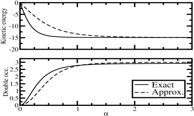
FIG. 1.: Kinetic and potential energies as a function of the variational parameter at half-filling.

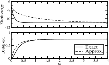
FIG. 2.: Kinetic and potential energies as a function of the variational parameter at quarter-filling.

In the limit $\alpha\rightarrow\infty$ the Hartree-Fock non-interacting ground state is obtained. In Eq. (22) the distribution in this limit includes only the ${\bf k}$ vectors corresponding to the lowest eigenvalues. Since the distribution corresponds to the finite temperature one with inverse temperature equal to $2\alpha$, it also follows that at half filling the discontinuity characterizing the Fermi surface of metals is only present when $\alpha\rightarrow\infty$. For the double occupations, only the ${\bf q}=0$ term survives when $\alpha\rightarrow\infty$. In the limiting cases $U=0$ and $U\rightarrow\infty$ the energies are correct within the present scheme, as is the case for the standard GA applied to the GWF. Generalization to systems away from half-filling is also straightforward, since the distribution for the $\alpha\rightarrow 0$ limit ($\chi({\bf k},{\bf l}$)) can be chosen accordingly.

D Application to the Baeriswyl-Gutzwiller wavefunction

It is also possible to generalize the above scheme to the combined projection based BGWF [9, 10] defined in Eq. (6 ). This generalization is enabled by the fact that the completely projected GWF on which the BWF is based (see Eqs. (2) and (3)) enters into the approximation scheme detailed in the previous subsection via the momentum density, which for the GA has a known form (Eq. (19)). Hence generalizing the approximation scheme to the BGWF proceeds exactly as described above, only that the momentum density is the one corresponding to the value of $\gamma$ (Eq. (19)).

E Implementation

In this work our implementation of the above approximations is similar to that described in Chapter 9 of Ref. [29]. Assuming that the distribution is fully uncorrelated in ${\bf k}$-space one can write the normalization as

$$\langle\Psi_{B}|\Psi_{B}\rangle\approx\prod_{{\bf k}\sigma}[1+\langle n_{{\bf k}\sigma}\rangle_{\gamma}\{\mbox{exp}(-2\alpha\epsilon({\bf k}))-1\}].$$ (28)

$\langle n_{{\bf k}\sigma}\rangle_{\gamma}$ is the momentum distribution of the Gutzwiller wavefunction (Eq. (19)). The kinetic energy is then obtained via

$$\sum_{{\bf k}\sigma}\epsilon({\bf k})\langle n_{{\bf k}\sigma}\rangle=-\frac{1}{2}\frac{\partial}{\partial\alpha}\mbox{ln}\langle\Psi_{B}|\Psi_{B}\rangle=\sum_{{\bf k}\sigma}\frac{\mbox{exp}(-2\alpha\epsilon({\bf k}))\epsilon({\bf k})\langle n_{{\bf k}\sigma}\rangle_{\gamma}}{1+\{\mbox{exp}(-2\alpha\epsilon({\bf k}))-1\}\langle n_{{\bf k}\sigma}\rangle_{\gamma}}.$$ (29)

The resulting interaction energy

$$U\sum_{i}\langle n_{i\uparrow}n_{i\downarrow}\rangle \approx U\frac{N_{\uparrow}N_{\downarrow}}{L}$$ (31)

$$+U\tilde{U}\sum_{{\bf k,k^{\prime},q}\neq 0}\frac{\mbox{exp}\{-\alpha(\epsilon({\bf k})+\epsilon({\bf k^{\prime}})-\epsilon({\bf k}+{\bf q})-\epsilon({\bf k^{\prime}}-{\bf q})\}(1-\langle n_{{\bf k}+{\bf q}\uparrow}\rangle_{\gamma})(1-\langle n_{{\bf k^{\prime}}-{\bf q}\downarrow}\rangle_{\gamma})\langle n_{{\bf k}\uparrow}\rangle_{\gamma}\langle n_{{\bf k^{\prime}}\downarrow}\rangle_{\gamma}}{C({\bf k},{\bf k^{\prime}},{\bf q})}$$

where

$$C({\bf k},{\bf k^{\prime}},{\bf q}) = (1+\langle n_{{\bf k}\sigma}\rangle_{\gamma}\{\mbox{exp}(-2\alpha\epsilon({\bf k}))-1\})(1+\langle n_{{\bf k^{\prime}}\sigma}\rangle_{\gamma}\{\mbox{exp}(-2\alpha\epsilon({\bf k^{\prime}}))-1\})$$ (33)

$$(1+\langle n_{{\bf k}+{\bf q}\sigma}\rangle_{\gamma}\{\mbox{exp}(-2\alpha\epsilon({\bf k}+{\bf q}))-1\})(1+\langle n_{{\bf k^{\prime}}+{\bf q}\sigma}\rangle_{\gamma}\{\mbox{exp}(-2\alpha\epsilon({\bf k^{\prime}}+{\bf q}))-1\}).$$

Note that the occupation factors in Eq. (31) are such that states ${\bf k}$ and ${\bf k^{\prime}}$ are occupied, and ${\bf k}+{\bf q}$ and ${\bf k^{\prime}}-{\bf q}$ are unoccupied, which coincide with the correlated hoppings in ${\bf k}$-space corresponding to the double occupation operator.

III Results

In Figs. 1 and 2 the kinetic and interaction energies are shown for a twelve site system comparing the results of an exact calculation to the outcome of the approach presented here for half and quarter fillings. The kinetic energy shows strong disagreement for intermediate values of the variational parameter, presumably due to the fact that this approach does not take into account momentum space correlations. The double occupations are in good agreement between the two calculations in both cases. A similar degree of agreement is found at quarter filling. Further testing of the method can be seen in Fig. 3 where the energy at half-filling is compared to the exact result [18], the exact Gutzwiller result [16, 17] and the Gutzwiller approximation applied to the GWF at half-filling. The discontinuity in the GA-B results indicates a first-order metal-insulator transition at $U_{c}\approx 4.04$, where the $U<U_{c}$ phase corresponds to $\alpha\rightarrow\infty$, the Hartree-Fock solution.

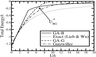
FIG. 3.: Comparison of the energy of the GA-B scheme to well known results: GA-G (Gutzwiller approximation applied to the GWF), exact Gutzwiller, and exact results. $U^{*}_{BG}$ indicates the transition point for the Baeriswyl-Gutzwiller wavefunction.

In Fig. 4 the phase diagram is presented calculated using $200$ sites. As the density decreases from half-filling, the critical interaction strength increases until it reaches a maximum. Similar behaviour is found when the density is increased from half-filling. In Fig. 5 the fraction of doubly occupied sites are shown as a function of the interaction strength at different fillings. For the half-filling case (shown in both panels) double occupations starts at one quarter (Hartree-Fock value), and then decreases abruptly at $U_{c}$. Subsequently it decays to zero with increasing $U$. This transition ”mirrors” the Brinkman-Rice [27] transition. There, while approaching the critical interaction from the metallic side, the number of double occupations decreases. The insulator of the Brinkman-Rice transition is the simplest possible insulator, with no double occupations. In the GA-B the double occupations increase when approaching the critical interaction from the insulating side, and the metallic side corresponds to the simplest metal; the non-interacting Hartree-Fock ground state.

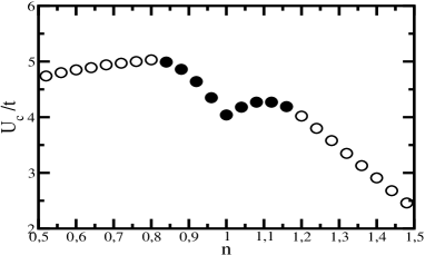
FIG. 4.: Critical interaction strength as a function of particle density. Closed circles indicate systems in which the large interaction phase contains bound excitons.

Fig. 5 also shows how the fraction of double occupied sites vary for different fillings. For $n<1$, close to half-filling the double occupations show the same pattern as for half-filling, until at $n\approx 0.8$ the state corresponding to large interaction strength no longer contains doubly occupied sites. Above half-filling there is a minimum fraction of doubly occupied sites for each system, but close to half-filling we observe a slow tending to the large $U$ limiting value (for example $n=1.08$). The fraction of doubly occupied sites above the limiting value are due to bound excitons, as they would not arise were it not for the Baeriswyl projector. Such bound excitons were only found in the range $n=0.8\leq n\leq 1.20$.

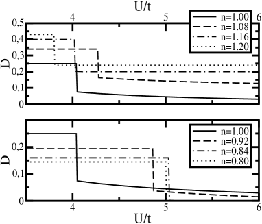
FIG. 5.: Double occupation as a function of interaction strength for various fillings.

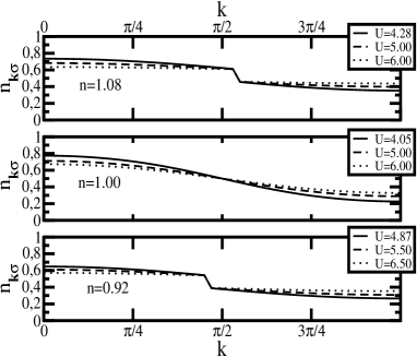
FIG. 6.: Density as a function of $k$-vector at different fillings for various values of the interaction strength.

In Fig. 6 the momentum density $n_{{\bf k}\sigma}$ is shown for different fillings as a function of $U$ in the phase corresponding to large $U$ in each case. The phases found at small $U$ have a Fermi step of $1$ at $\pi/2$. The Fermi step closes entirely for the system at half-filling, but remains finite for both systems away from half-filling. Thus away from half-filling, we find a a first order phase transition from an uncorrelated metallic phase to a metallic phase which contains bound excitons.

For the Baeriswyl-Gutzwiller projection the approximate scheme presented here results in a minimum energy corresponding either to the Gutzwiller or the Baeriswyl wavefunction. For half-filling the transition occurs between a correlated metal and a correlated insulator. The interaction strength at which the transition occurs is given by the crossing point of the energy curves GA-G and GA-B, and is indicated in Fig. 3 ($U^{*}_{BG}\approx 6.6$). Away from half-filling the interaction strength at which the transition occurs increases, and for $n=0.96$ we find no transition in the range $0\leq U\leq 20$: the ground state of the system is a partially projected Gutzwiller function( no bound excitons). For $n=0.98$ a first order phase transition is found. The transition occurs at $U^{*}_{BG}\approx 7.9$. For smaller values of the interaction the wavefunction is a partially projected Gutzwiller function, the Baeriswyl projection parameter ($\alpha$) is always zero, only the Gutzwiller parameter ($\gamma$) varies: the system is a correlated metal without bound excitons. For larger values of $U$ the parameter $\alpha$ is finite and approaches zero as $U\rightarrow\infty$. The Gutzwiller parameter is such that all double occupations are projected out for $\alpha=0$, and is constant in this range of $U$. In Fig. (7) the double occupation is shown as a function of the interaction strength. The double occupation decreases linearly for the correlated metal described by the Gutzwiller approximation, and is discontinuous at the phase transition. For the large interaction the double occupation decays to zero. In the regime where $\alpha$ and the double occupation is finite the double occupations can be attributed to bound excitons. Hence away from half-filling a metal-metal transition is found between two correlated metallic states, distinguished by the absence or presence of bound excitons.

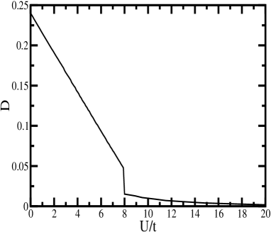
FIG. 7.: Double occupation as a function of interaction strength for the Baeriswyl-Gutzwiller wavefunction for filling $n=0.98$.

IV Conclusion

In summary, an approximate scheme was presented to solve the Baeriswyl and Baeriswyl-Gutzwiller variational wavefunctions. The approach presented here is simple and easy to apply in finite dimensional systems and large system sizes are tractable. The scheme is similar in spirit to the well-known Gutzwiller approximation, in which the starting point is the Fermi sea, and the Pauli principle is implemented by requiring that no two particles of the same spin can be on the same site in real space, but no other spin correlation effects are included. In the approach described herein two particles of the same spin cannot occupy the same site in ${\bf k}$-space, hence an approximate treatment of the ${\bf k}$-space analog of the exchange hole is developed.

At half-filling a metal-insulator transition is found, where the metallic phase ($U<U_{c}$) corresponds to the Hartree-Fock solution, the insulating phase is one with finite double occupations corresponding to bound excitons. This transition can be viewed as the ”inverse” of the Brinkman-Rice transition. Close to but away from half filling, the $U>U_{c}$ phase displays a finite Fermi step (metallic), as well as double occupations originating from bound excitons. As the filling is increased or decreased from half-filling bound excitons are supressed.

For the Baeriswyl-Gutzwiller wavefunction it was found that the optimal solution is always either the Baeriswyl or the Gutzwiller wavefunction in this approximate scheme. The phase transitions shift to larger values of the interaction strength. At half-filling a metal-insulator transition occurs between a correlated metal (with double occupations suppressed) and a correlated insulator (double occupations arising from bound excitons). Away from, but still close to, half-filling a transition was found between two metallic phases, the correlated metallic state arising from the Gutzwiller approximation for small interaction, and one containing double occupations arising from exciton binding for large interaction.

- [1] M. C. Gutzwiller, Phys. Rev. Lett., 10 159 (1963).
- [2] M. C. Gutzwiller, Phys. Rev., 137 A1726 (1965).
- [3] J. Hubbard, Proc. R. Soc. London, A276 238 (1963).
- [4] J. Kanamori, Prog. Theoret. Phys., 30 275 (1963).
- [5] A. Georges, G. Kotliar, W. Krauth, and M. J. Rozenberg , Rev. Mod. Phys., 68 13 (1996).
- [6] U. Schollwöck, Rev. Mod. Phys., 77 259 (2005).
- [7] D. Baeriswyl in Nonlinearity in Condensed Matter, Ed. A. R. Bishop, D. K. Campbell, D. Kumar, and S. E. Trullinger, Springer-Verlag (1986).
- [8] D. Baeriswyl, Found. Physics, 30 2033 (2000).
- [9] H. Otsuka, J. Phys. Soc. Japan, 61 1645 (1992).
- [10] M. Dzierzawa, D. Baeriswyl, M. DiStasio, Phys. Rev. B, 51 1993 (1995).
- [11] D. Baeriswyl, D. Eichenberger and M. Menteshashvili, New J. Phys., 11 075010 (2009).
- [12] D. Eichenberger and D. Baeriswyl, Phys. Rev. B, 79 100510 (2009).
- [13] S. Vitiello, K. M. Runge, and M. H. Kalos, Phys. Rev. Lett., 60 1970 (1988).
- [14] B. Hetényi, E. Rabani, and B. J. Berne, J. Chem. Phys., 110 6143 (1999).
- [15] A. Sarsa, K. E. Schmidt, W. R. Magro, J. Chem. Phys., 113 1366 (2000).
- [16] W. Metzner and D. Vollhardt Phys. Rev. Lett., 59 121 (1987).
- [17] W. Metzner and D. Vollhardt, Phys. Rev. Lett., 62 324 (1989).
- [18] E. H. Lieb and F. Y. Wu, Phys. Rev. Lett., 20 1445 (1968).
- [19] A. J. Millis and S. N. Coppersmith, Phys. Rev. B, 43 13770 (1991).
- [20] M. Dzierzawa, D. Baeriswyl, and L. M. Martelo, Helv. Phys. Acta, 70 124 (1997).
- [21] Z. Gulácsi, M. Gulácsi, and B. Jankó Phys. Rev. B 47 4168 (1993).
- [22] H. Yokoyama and H. Shiba, J. Phys. Soc. Japan, 56 1490 (1987).
- [23] M. Capello, F. Becca, M. Fabrizio, S. Sorella, and E. Tosatti, Phys. Rev. Lett., 94 026406 (2005).
- [24] D. Tahara and M. Imada, J. Phys. Soc. Jpn., 77 093703 (2008).
- [25] M. Kollar and D. Vollhardt, Phys. Rev. B, 63 045107(2001).
- [26] M. Kollar and D. Vollhardt, Phys. Rev. B, 65 155121 (2002).
- [27] W. F. Brinkman and T. M. Rice, Phys. Rev. B, 2 4302 (1970).
- [28] D. Vollhardt, Rev. Mod. Phys., 56 99 (1984).
- [29] P. Fazekas, Lecture Notes on Electron Correlation and Magnetism, World Scientific (1999).
- [30] B. Edegger, V. N. Muthukumar, and C. Gros, Adv. Phys., 56 927 (2007).
- [31] J. Kurzyk, J. Spałek, and W. Wójcik, Acta Phys. Polonica A 111 603 (2007).
- [32] B. Hetényi, H. G. Evertz, and W. von der Linden, Phys. Rev. B 80 045107 (2009).
- [33] F. Lado, J. Chem. Phys., 47 5369 (1967).
- [34] F. A. Stevens and M. A. Pokrant, Phys. Rev. A, 8 990 (1967).
- [35] B. Hetényi, L. Brualla, and S. Fantoni Phys. Rev. Lett., 93 170202 (2004).
- [36] B. Hetényi and A. W. Hauser Phys. Rev. B, 77 155110 (2008).
- [37] G. Seibold and J. Lorenzana, Phys. Rev. Lett., 86 2605 (2001).
- [38] J. Bünemann, D. Rasch, and F. Gebhard, J. Phys. Condens. Matter, 19 436206 (2007).
- [39] B. Edegger, N. Fukushima, C. Gros, and V. N. Muthukumar, Phys. Rev. B, 72 134504 (2005).
- [40] N. Fukushima, B. Edegger, V. N. Muthukumar, and C. Gros, Phys. Rev. B, 72 144505 (2005).
- [41] H. Heiselberg Phys. Rev. A, 79 063611 (2009).
- [42] L. Wang, X. Dai, S. Chen, and X. C. Xie, Phys. Rev. A, 78 023603 (2008).
- [43] J. Qi, L. Wang, and X. Dai, Chinese Phys. Lett. 27 083102 (2010).
- [44] X. Y. Deng, X. Dai, and Z. Fang, Europhys. Lett., 83 37008 (2008).
- [45] X. Y. Deng, L. Wang, X. Dai, and Z. Fang, Phys. Rev. B, 79 075114 (2009).
- [46] G. T. Wang, Y. Qian, G. Xu, X. Dai, and Z. Fang, Phys. Rev. Lett., 104 047002 (2010).
- [47] G. Seibold, F. Becca, P. Rubin, and J. Lorenzana, Phys. Rev. B, 69 155113 (2004).
- [48] A. Di Ciolo, J. Lorenzana, M. Grilli, and G. Seibold, Phys. Rev. B, 79 085101 (2009).
- [49] R. S. Markiewicz, J. Lorenzana, G. Seibold, and A. Bansil, Phys. Rev. B, 81 014509 (2010).
- [50] R. S. Markiewicz, J. Lorenzana, and G. Seibold, Phys. Rev. B, 81 014510 (2010).
- [51] J. Jedrak, J. Kaczmarczyk, and J. Spałek, arXiv:2010.0021.
- [52] F. C. Zhang, C. Gros, T. M. Rice, and H. Shiba, Supercond. Sci. Tech., 1 36 (1988).
- [53] B. Edegger, V. N. Muthukumar, C. Gros, and P. W. Anderson, Phys. Rev. Lett., 96 207002 (2006).
- [54] C. Gros, B. Edegger, V. N. Muthukumar, and P. W. Anderson, Proc. Nat. Acad. Sci. USA, 103 14298 (2006).
- [55] P. W. Anderson, Mater. Res. Bull., 8 153 (1973).
- [56] P. Fazekas and P. W. Anderson, Phil. Mag., 30 432 (1974).
- [57] P. W. Anderson, P. A. Lee, M. Randeria, T. M. Rice, N. Trivedi, and F. C. Zhang, J. Phys. Condens. Matter, 16 R755 (2004).
- [58] C. D. Spataru, S. Ismail-Beigi, L. X. Benedict, and S. G. Louie, Phys. Rev. Lett., 92 077402 (2004).
- [59] F. Wang, D. J. Cho, B. Kessler, J. Deslippe, P. J. Schuck, S. G. Louie, A. Zettl, T. F. Heinz, and Y. R. Shen Phys. Rev. Lett., 99 227401 (2007).