Population III GRB Afterglows:
Constraints on Stellar Masses and External Medium Densities

Abstract

Population III stars are theoretically expected to be prominent around redshifts $z\sim 20$, consisting of mainly very massive stars with $M_{*}\gtrsim 100\;M_{\odot}$, but there is no direct observational evidence for these objects. They may produce collapsar gamma-ray bursts (GRBs), with jets driven by magnetohydrodynamic processes, whose total isotropic-equivalent energy could be as high as $E_{\rm iso}\gtrsim 10^{57}\;$erg over a cosmological-rest-frame duration of $t_{d}\gtrsim 10^{4}\;$s, depending on the progenitor mass. Here we calculate the afterglow spectra of such Pop. III GRBs based on the standard external shock model, and show that they will be detectable with the Swift BAT/XRT and Fermi LAT instruments. We find that in some cases a spectral break due to electron-positron pair creation will be observable in the LAT energy range, which can put constraints on the ambient density of the pre-collapse Pop. III star. Thus, high redshift GRB afterglow observations could be unique and powerful probes of the properties of Pop. III stars and their environments. We examine the trigger threshold of the BAT instrument in detail, focusing on the image trigger system, and show that the prompt emission of Pop. III GRBs could also be detected by BAT. Finally we briefly show that the late-time radio afterglows of Pop. III GRBs for typical parameters, despite the large distances, can be very bright: $\simeq 140\;$mJy at $1\;$GHz, which may lead to a constraint on the Pop. III GRB rate from the current radio survey data, and $\simeq 2.4\;$mJy at $70\;$MHz, which implies that Pop. III GRB radio afterglows could be interesting background source candidates for 21 cm absorption line detections.

1. Introduction

Recent studies on cosmology and primordial star formation predict that the first generation of stars (population III stars) may be most prominent around $z\sim 20$, consisting of metal-poor, mainly very massive stars (VMSs) with $M_{*}\gtrsim 100\;M_{\odot}$ (e.g., Abel et al., 2002; Omukai & Palla, 2003; Yoshida et al., 2006; Ciardi & Ferrara, 2005). These first stars are thought to play a significant role in setting off cosmic reionization, in the initial enrichment of the intergalactic medium (IGM) with heavy elements, and in seeding the intermediate and supermassive black holes (BHs) encountered in galaxies. The details of how these processes unfold remain elusive, since observational data for redshifts $z\gtrsim 6$ are very limited.

Observations of gamma-ray bursts (GRBs), however, may provide unique probes of the physical conditions of the universe at such redshifts. The GRB prompt emission and the afterglows were expected to be observable at least out to $z\gtrsim 10$, with their redshifts being determined through the detection of a Ly$\alpha$ drop-off in the infrared (IR), or through redshifted atomic lines back-lighted by the afterglows (e.g., Lamb & Reichart, 2000; Ciardi & Loeb, 2000; Gou et al., 2004). This can serve as a tracer of the history of the cosmic star formation rate (e.g., Totani, 1997; Porciani & Madau, 2001; Bromm & Loeb, 2006; Kistler et al., 2009), providing invaluable information about the physical conditions in the IGM of the very high redshift universe (e.g., Barkana & Loeb, 2004; Ioka & Mészáros, 2005; Inoue et al., 2006). Currently the most distant object that has been spectroscopically confirmed is GRB 090423 at $z\simeq 8.2$ (Tanvir et al., 2009; Salvaterra et al., 2009), and the detailed spectroscopic observation of GRB 050904 at $z\simeq 6.3$ has put a unique upper bound on the neutral hydrogen fraction in the IGM at that redshift (Totani et al., 2006; Kawai et al., 2006), indicating that GRB observations are very promising for exploring the high-redshift universe (see also Greiner et al., 2009, for GRB 080913 with $z\simeq 6.7$).

In those previous papers, the GRBs arising from Population III VMSs were considered to have similar properties as the GRBs arising from Population I/II stars, e.g., they were usually assumed to have similar luminosity functions, even if perhaps extending to somewhat higher masses, and most importantly, their radiation properties, durations and spectra were modeled as being essentially similar to their lower redshift counterparts. However, this simplifying assumption may not be valid, as pointed out by Fryer et al. (2001) and Komissarov & Barkov (2010) (hereafter KB10). One difference is that the accretion disks around the much larger black holes resulting from core collapse of VMS progenitor would be too cool to lead to neutrino-cooled thin disks and conversion of neutrinos into electron-positron pairs (Eichler et al., 1989; Woosley, 1993). Thus, the Pop. III GRBs are much likelier to be driven by MHD processes, converting the rotational energy of the central BH into a Poynting-flux-dominated jet (Blandford & Znajek, 1977), rather than the usually assumed thermal-energy-dominated jets. The total energy of a Pop. III GRB is then proportional to the total disk (torus) mass, which in turn can be assumed to be proportional to the progenitor stellar mass, which can be much higher than that of a Pop. I/II GRB. In addition, the fall-back time and/or the disk accretion time, i.e., the active duration time of a Pop. III GRB jet can be much longer than that of a Pop. I/II GRB jet, due to the larger progenitor star.

Building on this premise, Mészáros & Rees (2010) (hereafter MR10) proposed a possible model of the prompt emission and afterglow of such Pop. III GRBs, and made rough predictions for their observational properties in the Swift and Fermi satellite bands. In this paper, we calculate in significantly more detail the very early afterglow properties of Pop. III GRBs, and show that the combination of Swift and Fermi observations, complemented by deep IR observations of the afterglow immediately following the prompt emission, can constrain the total isotropic-equivalent energies $(E_{\rm iso})$ of the Pop. III GRBs, as well as the particle densities $n$ of their circumburst medium. The detection of a burst with a very high total isotropic-equivalent energy $E_{\rm iso}\gtrsim 10^{57}\;$erg and a very long (cosmological rest frame) duration $t_{d}\gtrsim 10^{4}\;$s would be strong evidence for a VMS progenitor. To constrain the total energy and the duration, observations of the prompt emission, whose interpretation is more dependent on the model details, should be complemented with observations of the afterglow, which is much less model-dependent.

The properties of the circumburst medium, i.e., the environments of the first stars prior to their collapse, have so far only been inferred from model numerical simulations, which differ significantly among each other. For example, the typical galactic gas environment could evolve as $n\propto(1+z)^{4}$ (Ciardi & Loeb, 2000), or it might be approximately independent of redshift, $n\sim 0.1\;{\rm cm}^{-3}$, as a result of stellar radiation feedback (Whalen et al., 2004; Alvarez et al., 2006). Observations and modeling of high-redshift GRB afterglows could distinguish between such numerical models. The small number of analyses of what are currently the most distant GRBs imply that the circumburst densities of these high-redshift GRBs could be very different from each other, e.g. $n\simeq 10^{2}-10^{3}\;{\rm cm}^{-3}$ for GRB 050904 with $z\simeq 6.3$ (Gou et al., 2007), and $n\simeq 1\;{\rm cm}^{-3}$ for GRB 090423 with $z\simeq 8.2$ (Chandra et al., 2010). A high total energy and a high circumburst medium density could lead, in principle, to such a high compactness parameter of the shocked afterglow emission region that a spectral break due to $e^{+}e^{-}$ pair production (i.e., $\gamma\gamma$ self-absorption break) may be observable in the Fermi LAT energy range. This is a unique and interesting point, which we explore here, since the $\gamma\gamma$ self-absorption is usually not significant for the afterglows of Pop. I/II GRBs (Zhang & Mészáros, 2001). Using this, we could constrain the circumburst density $n$ from the observation of a $\gamma\gamma$ self-absorption break, which is a new method to constrain the environment of the pre-explosion GRB host galaxy.

The external shock model of the GRB afterglows seems to be robust, since it can explain many of the late-time multi-band afterglows detected so far, and a simple extension of this model (e.g., continuous energy injection into the external shock) may explain many of the early-time (observer’s time $t_{\rm obs}\lesssim 1\;$hr) X-ray and optical afterglows detected by Swift (Liang et al., 2007). More importantly, some of the very early high-energy afterglows (immediately following the prompt emission) recently observed by Fermi LAT are shown to be explained by this model (e.g., Kumar & Barniol Duran, 2009; De Pasquale et al., 2010; Corsi et al., 2010).

The basic parameters of the Poynting-dominated Pop. III GRB model are defined in Section 2. The very early afterglow spectrum is calculated in Section 3 (based on the standard external shock model described in Appendix), where we discuss how to constrain $E_{\rm iso},t_{d}$ and $n$ from the observations. In Section 4 we deduce the effective trigger threshold of the Swift BAT instrument, and show that the prompt emission of Pop. III GRBs could trigger BAT. In Section 5 we compute the late-time radio afterglow flux for a typical set of parameters, and evaluate the current radio survey data constraints on the Pop. III GRB rate, as well as the prospects for 21 cm absorption line detection in the Pop. III GRB radio afterglow spectra. In Section 6 we present a summary of our findings.

2. Poynting-dominated Pop. III GRB Model

We consider VMSs rotating very fast, close to the break-up speed, as a representative case of Pop. III GRB progenitor stars. Those in the $140\;M_{\odot}\lesssim M_{*}\lesssim 260\;M_{\odot}$ range are expected to explode as pair instability supernovae without leaving any compact remnant behind, while those in the $M_{*}\gtrsim 260\;M_{\odot}$ range are expected to undergo a core collapse leading directly to a central BH, whose mass would itself be hundreds of solar masses (Fryer et al., 2001; Heger et al., 2003; Ohkubo et al., 2006). Accretion onto such BHs could lead to collapsar GRBs (Woosley, 1993; MacFadyen & Woosley, 1999). Prior to the collapse, the fast rotating VMSs may be chemically homogeneous and compact, without entering the red giant phase, so that the stellar radius is $R_{*}\simeq 10^{12}\;$cm for $M_{*}\simeq 10^{3}\;M_{\odot}$ (KB10; Yoon et al., 2006; Woosley & Heger, 2006).

For such large BH masses $M_{h}\gtrsim 100M_{\odot}$, the density and temperature of the accretion disk are too low for neutrino cooling to be important, and the low neutrino release from the accretion disk is insufficient to power a strong jet (Fryer et al., 2001). The rate of energy deposition through this mechanism may be estimated by using the formula recently deduced by Zalamea & Beloborodov (2010)

$$L_{\nu\bar{\nu}}\simeq 5\times 10^{46}\;\dot{M}_{-1}^{9/4}M_{h,2.5}^{-3/2}\;{\rm erg}\;{\rm s}^{-1},$$ (1)

where $\dot{M}=0.1\dot{M}_{-1}M_{\odot}\;{\rm s}^{-1}$ is the accretion rate and $M_{h,2.5}=M_{h}/(10^{2.5}M_{\odot})$. This is clearly insufficient for detection from such high redshifts. However, strong magnetic field build-up in the accretion torus or disk could lead to much stronger jets, dominated by Poynting flux. Such jets will be highly relativistic, driven by the magnetic extraction of the rotational energy of the central BH through the Blandford-Znajek (BZ) mechanism (Blandford & Znajek, 1977). The luminosity extracted from a Kerr BH with dimensionless spin parameter $a_{h}$ threaded by a magnetic field of strength $B_{h}$ is (Thorne et al., 1986)

$$L_{\rm BZ}\approx\frac{a_{h}^{2}}{128}B_{h}^{2}R_{h}^{2}c,$$ (2)

where $R_{h}\approx GM_{h}/c^{2}$ is the event horizon radius of the BH. The dynamics of the radiatively inefficient accretion disk may be described (KB10) through advection-dominated (ADAF) model (Narayan & Yi, 1994). For a VMS rotating at, say, half the break-up speed, the disk outer radius will be $R_{d}\simeq R_{*}/4$, and for a disk viscosity parameter $\alpha=10^{-1}\alpha_{-1}$, the accretion time is

$$t_{d}\simeq\frac{7}{3\alpha}\left({\frac{R_{d}^{3}}{GM_{h}}}\right)^{1/2}\simeq 1.4\times 10^{4}\;\alpha_{-1}^{-1}R_{*,12}^{3/2}M_{h,2.5}^{-1/2}\;{\rm s},$$ (3)

where we have defined $R_{*,12}=R_{*}/10^{12}\;{\rm cm}$. This gives an estimate for both the disk lifetime and the duration of the jet, in the source frame. Given the jet propagation speed inside the star, $\sim 0.2c$, deduced from magnetohydrodynamic simulations (Barkov & Komissarov, 2008), the intrinsic jet duration $t_{d}\simeq 10^{4}\;$s is sufficient to break through the star. The poloidal magnetic field strength in the disk should scale with the disk gas pressure, $P$, so that $B_{h}^{2}=8\pi P/\beta$, where $\beta=10\;\beta_{1}$ is the magnetization parameter (e.g., Reynolds et al., 2006). Then we have

$$B_{h}\simeq\left(\frac{4\sqrt{14}}{3\alpha\beta}\frac{\dot{M}c}{R_{h}^{2}}\right)^{1/2}\simeq 6.6\times 10^{13}\;\frac{1}{\alpha_{-1}\beta_{1}}M_{h,2.5}^{-1}M_{d,2.5}^{1/2}t_{d,4}^{-1/2}\;{\rm G}.$$ (4)

Combining these equations result in a jet luminosity

$$L_{\rm BZ}\simeq\frac{\sqrt{14}}{96}\frac{a_{h}^{2}}{\alpha\beta}\dot{M}c^{2}\simeq 2.2\times 10^{51}\;\frac{a_{h}^{2}}{\alpha_{-1}\beta_{1}}M_{d,2.5}t_{d,4}^{-1}\;{\rm erg}\;{\rm s}^{-1},$$ (5)

where for the second equalities in Eqs. (4) and (5) we have assumed a constant accretion rate $\dot{M}\simeq M_{d}/t_{d}$, and $M_{d}=10^{2.5}M_{d,2.5}M_{\odot}$ is the total disk mass.

Let us assume that the factor $a_{h}^{2}/(\alpha\beta)$ is roughly constant, so that $L_{\rm BZ}\propto\dot{M}$. The total extracted energy during the accretion time $t_{d}$ is then $E_{\rm BZ}\simeq(\sqrt{14}/96)(a_{h}^{2}/\alpha\beta)M_{d}c^{2}$. Assuming that the jet has an opening angle of $\theta_{j}=0.1\;\theta_{j,-1}$, we can then write the total isotropic-equivalent energy of the jet as

$$E_{\rm iso}\simeq 4.4\times 10^{57}\;\frac{(1-\epsilon_{\gamma})a_{h}^{2}}{\alpha_{-1}\beta_{1}}M_{d,2.5}\theta_{j,-1}^{-2}\;{\rm erg},$$ (6)

where $\epsilon_{\gamma}$ is the radiation efficiency of the prompt emission, and $1-\epsilon_{\gamma}$ is of order of unity. Equation (6) is also applicable to cases where $\dot{M}$ is not constant. As far as $L_{\rm BZ}\propto t^{-q}$ (i.e., $\dot{M}\propto t^{-q}$) with $q\leq 1$, the jet can break out from the star and subsequently keep injecting energy into the external medium for the duration of the order of $t_{d}$. The forward shock produced in the external medium enters a self-similar expansion phase with total shock energy $\simeq E_{\rm iso}$ soon after $t=t_{d}$ (Blandford & McKee, 1976). Interestingly, the value of $E_{\rm iso}$ for a disk mass $M_{d}\sim 3\;M_{\odot}$ is consistent with the observed largest value of the isotropic-equivalent $\gamma$-ray energy $E_{\gamma,{\rm iso}}\simeq 10^{55}\;$erg for GRB 080916C at the redshift $z\simeq 4.4$ (Abdo et al., 2009). (On the other hand, the isotropic luminosity $L_{\rm iso}\simeq 4.4\times 10^{53}\;(a_{h}^{2}/\alpha\beta)M_{d,2.5}t_{d,4}^{-1}\theta_{j,-1}^{-2}\;{\rm erg}\;{\rm s}^{-1}$ is comparable to the observed largest value.) Thus, if we were to observe a burst at redshift $z\gtrsim 10$ with $E_{\rm iso}\gtrsim 10^{57}\;$erg, and with a self-similar phase starting at $t_{d,{\rm obs}}=t_{d}(1+z)\gtrsim 1\;$day, this would very likely be a burst from a Pop. III VMS with $M_{*}\gtrsim 300\;M_{\odot}$.

Figure 1.— Schematic figure of the bolometric luminosity evolutions of the external shock emission (thick line) and the prompt emission (thin line) as functions of time from the onset of the prompt emission. The prompt emission may involve some variability, which is shown by the dotted line. In this figure we assume that the jet luminosity $L_{\rm BZ}$ is constant for $t_{\rm obs}<t_{d,{\rm obs}}=t_{d}(1+z)$ and subsequently declines rapidly. The external shock is in the thick-shell regime. Its luminosity is also constant for $t_{\rm obs}<t_{d,{\rm obs}}$ and subsequently enters the self-similar phase $L\propto t_{\rm obs}^{-1}$. The argument is similar for the case of the jet luminosity $L_{\rm BZ}\propto t^{-q}$ with $q\leq 1$, where luminosities of the prompt emission and external shock emission both evolve as $L\propto t_{\rm obs}^{-q}$ before $t_{d,{\rm obs}}$ and in the same way as this figure after $t_{d,{\rm obs}}$.

3. Very Early Afterglow Spectrum

Rough predictions for the observational properties of the afterglows of Pop. III GRBs were made in MR10. The external shock driven by the jet in the circumburst medium powers the afterglow, which can be studied independently of the prompt emission (Mészáros & Rees, 1997a; Sari et al., 1998; Sari & Esin, 2001). This is true whether the jet is baryonic or Poynting-dominated, the jet acting simply as a piston. The external shock amplifies the magnetic field in the shocked region via plasma and/or magnetohydrodynamic instabilities, and accelerates the electrons in the shocked region to a power-law energy distribution. The accelerated electrons produce synchrotron and synchrotron-self-Compton (SSC) radiation as an afterglow. Here we go beyond the previous schematic outlines, and calculate the spectrum of this emission in detail, including the Klein-Nishina as well as $e^{+}e^{-}$ pair formation effects.

The bolometric luminosity of the external shock emission (with prompt emission light curve) is illustrated in Figure 1. We focus on the external shock emission at the observer’s time $t_{\rm obs}\simeq t_{d,{\rm obs}}$, near the beginning of the self-similar expansion phase of the shock, when the emission is bright and may not be hidden by the prompt emission.

Calculations of the external shock emission spectrum involve the parameters $E_{\rm iso}$ and $t_{d}$, as well as the external medium number density $n$, the fractions $\epsilon_{B}$ and $\epsilon_{e}$ of the thermal energy in the shocked region that are carried by the magnetic field and the electrons, respectively, and the index $p$ of the energy spectrum of the accelerated electrons. We calculate the external shock emission spectrum of a Pop. III GRB at $t_{d,{\rm obs}}$ based on the standard model described in Appendix.

As introduced in Section 1, the circumburst medium density in the very high-redshift universe is likely to be $n\gtrsim 0.1\;{\rm cm}^{-3}$. The microphysical parameters may be independent of $E_{\rm iso},t_{d},$ or $n$ as long as the shock velocity is highly relativistic, so that $\epsilon_{B},\epsilon_{e}$, and $p$ are thought to be similar to those for the bursts observed so far. Those have been constrained by fitting the late-time afterglows through models (which are similar to our model shown in Appendix). The parameters related to the electrons are constrained relatively tightly as $\epsilon_{e}\sim 0.1$ and $p\sim 2.3$, while those for the magnetic field are not so tightly constrained, although typically for many afterglows $10^{-3}\lesssim\epsilon_{B}\lesssim 10^{-1}$ (e.g., Panaitescu & Kumar, 2002; Wijers & Galama, 1999).

The external shock emission at $t_{d,{\rm obs}}$ will have two intrinsically different cases, depending on the significance of the electron-positron pair creation within the emitting region. These cases are characterized by a negligible pair production regime and a significant pair production regime, which we show examples of spectra separately below.

3.1. Case of Negligible Pair Production

Figure 2.— Example of the observer-frame spectrum of a Pop. III GRB at the time $t_{d,{\rm obs}}$ when the jet activity ends, for the case of negligible intra-source pair production. The parameters are $E_{57.6}=t_{d,4}=n_{0}=\epsilon_{B,-2}=\epsilon_{e,-1}=f(p)=1$, and the source redshift $1+z=20$. The dot-dashed line shows the external shock (afterglow) spectrum, which consists of the synchrotron and SSC components (solid lines). The synchrotron component peaks at $\varepsilon_{m}\simeq 5.4\;$eV, and the SSC component peaks at $\varepsilon_{m}^{\rm SC}\simeq 1.8\times 10^{2}\;$MeV. The $\gamma\gamma$ self-absorption break energy is $\varepsilon_{\gamma\gamma}\simeq 21\;$GeV, which is larger than the SSC peak $\varepsilon_{m}^{\rm SC}$, so that most of the SSC emission escapes without being absorbed within the emitting region. The $\gamma\gamma$ absorption due to the EBL is expected to become significant at $\varepsilon>\varepsilon_{\rm EBL}\simeq 7\;$GeV (Inoue et al., 2010), as shown by the dashed line. The dotted line represents the prompt emission’s dominant photospheric black-body component with a possible power-law extension, assuming $1+\sigma=10$ and $L_{53.6}=r_{l,8}=\Gamma_{l}=1$ (see Section 4.2).

An example of the negligible pair production case is obtained for the parameters

$$E_{57.6}=t_{d,4}=n_{0}=\epsilon_{B,-2}=\epsilon_{e,-1}=f(p)=1,$$ (7)

where the notation $Q=10^{x}Q_{x}$ in cgs units has been adopted ($E_{57.6}=E_{\rm iso}/10^{57.6}\;{\rm erg}$). The overall observer-frame spectrum for this case is shown in Figure 2 (see Appendix A.1). The synchrotron emission spectrum peaks at $\varepsilon_{m}\simeq 5.4\;$eV with the flux $\varepsilon_{m}F_{\varepsilon_{m}}\simeq 4.4\times 10^{-10}\;{\rm erg}\;{\rm cm}^{-2}\;{\rm s}^{-1}$, having spectral breaks at synchrotron self-absorption energy $\varepsilon_{a}\simeq 9.7\times 10^{-4}\;$eV and at energy corresponding to the maximum electron energy $\varepsilon_{M}\simeq 1.8\times 10^{2}\;$MeV. The SSC emission spectrum peaks at $\varepsilon_{m}^{\rm SC}\simeq 1.8\times 10^{2}\;$MeV with the flux $\varepsilon_{m}^{\rm SC}F_{\varepsilon_{m}}^{\rm SC}\simeq 1.2\times 10^{-9}\;{\rm erg}\;{\rm cm}^{-2}\;{\rm s}^{-1}$ and has a spectral break at $\gamma\gamma$ self-absorption energy $\varepsilon_{\gamma\gamma}\simeq 21\;$GeV. Since $\varepsilon_{\gamma\gamma}>\varepsilon_{m}^{\rm SC}$, most of the SSC emission is observed without being converted into $e^{+}e^{-}$ within the emitting region.

Even photons escaping without attenuation within the emitting region can be absorbed by interacting with the extragalactic background light (EBL) ($\gamma\gamma\to e^{+}e^{-}$). Inoue et al. (2010) use a semi-analytic model of the evolving EBL and expect that high-energy photon absorption by the EBL for an arbitrary source at $z\simeq 20$ is significant at $\varepsilon>\varepsilon_{\rm EBL}\simeq 7\;$GeV. For the parameters adopted here, $\varepsilon_{\gamma\gamma}$ is larger than $\varepsilon_{\rm EBL}$, which precludes obtaining intrinsic information about the emitting region from the observation of the $\gamma\gamma$ break.

The temporal evolution of the characteristic quantities during the self-similar phase, i.e., at $t_{\rm obs}>t_{d,{\rm obs}}$ is obtained replacing $t_{d}$ by the variable $t_{\rm obs}$ in the model equations in Appendix, and taking all other parameters as constant. On the other hand, for $t_{\rm obs}<t_{d,{\rm obs}}$, if the jet luminosity evolves as $L_{\rm BZ}\propto t^{-q}$ with $q\leq 1$, one can obtain the temporal evolution of the characteristic quantities by taking $E_{\rm iso}\propto t_{\rm obs}^{1-q}$, replacing $t_{d}$ by $t_{\rm obs}$, and taking all the other parameters as constant. In the high-energy range, $\varepsilon_{m}^{\rm SC}<\varepsilon<\varepsilon_{\gamma\gamma}$, as an example, we obtain $F^{\rm SC}_{\varepsilon_{m}^{\rm SC}<\varepsilon<\varepsilon_{\gamma\gamma}}\propto t_{\rm obs}^{(3/4)(2-p)-(3/8)q(p+2/3)}$ for $t_{\rm obs}<t_{d,{\rm obs}}$, and $\propto t_{\rm obs}^{(10-9p)/8}$ for $t_{\rm obs}>t_{d,{\rm obs}}$, which implies a steepening break at $t_{d,{\rm obs}}$ for $p\sim 2$ and $q<1$. Thus one can identify the jet duration $t_{d,{\rm obs}}$ as the observed break time. (One can also estimate $t_{d,{\rm obs}}$ by the duration of the prompt emission.)

3.2. Case of Significant Pair Production

Figure 3.— Example of a Pop. III GRB spectrum at time $t_{d}$ with significant pair production in the external shock. The parameters are $E_{57.6}=t_{d,4}=\epsilon_{B,-2}=f(p)=1$, $n=10^{2}$, and $\epsilon_{e,-1}=2$, and the source redshift $1+z=20$. The dot-dashed line shows the external shock emission spectrum, which consists of the four components (solid lines). The synchrotron component of the original electrons peaks at $\varepsilon_{m}\simeq 21\;$eV. The peak of the SSC emission of the original electrons (not shown in this figure) $\varepsilon_{m}^{\rm SC}\simeq 9.2\times 10^{2}\;$MeV is above the $\gamma\gamma$ self-absorption break energy $\varepsilon_{\gamma\gamma}\simeq 6.1\times 10^{2}\;$MeV, so that most of the SSC emission is absorbed within the emission region. The pairs emit synchrotron and SSC radiations peaking at $\varepsilon_{\pm,p}\simeq 0.11\;$eV and $\varepsilon_{\pm,p}^{\rm SC}\simeq 23\;$keV, respectively. The IC-scattered original synchrotron emission by the pairs and the IC-scattered pair synchrotron emission by the original electrons have spectra with similar characteristic energies (including the peak energies at $\varepsilon_{m}^{\rm IC}=\varepsilon_{\pm,p}^{\rm IC}\simeq 4.5\;$MeV) and different flux normalizations, which have been superposed in this figure. The $\gamma\gamma$ absorption due to the EBL is expected to be significant above $\simeq 7\;$GeV (Inoue et al., 2010), as shown by the dashed line. The dotted line represents the prompt emission’s dominant photospheric black-body component with a possible power-law extension, assuming $1+\sigma=10$ and $L_{53.6}=r_{l,8}=\Gamma_{l}=1$ (see Section 4.2).

An example of the case of significant pair production is obtained with the parameter set

$$E_{57.6}=t_{d,4}=\epsilon_{B,-2}=f(p)=1,~{}~{}~{}n_{0}=10^{2},~{}~{}~{}\epsilon_{e,-1}=2.$$ (8)

The overall observer-frame spectrum for this case is shown in Figure 3 (see Appendix A.2). The synchrotron emission spectrum of the original electrons peaks at $\varepsilon_{m}\simeq 21\;$eV with the flux $\varepsilon_{m}F_{\varepsilon_{m}}\simeq 5.8\times 10^{-10}\;{\rm erg}\;{\rm cm}^{-2}\;{\rm s}^{-1}$, having the maximum energy $\varepsilon_{M}\simeq 1.0\times 10^{2}\;$MeV. The $\gamma\gamma$ self-absorption energy is $\varepsilon_{\gamma\gamma}\simeq 6.1\times 10^{2}\;$MeV, and thus most of the SSC emission with the spectral peak $\varepsilon_{m}^{\rm SC}\simeq 9.2\times 10^{2}\;$MeV with the peak flux $\varepsilon_{m}^{\rm SC}F_{\varepsilon_{m}}^{\rm SC}\simeq 2.7\times 10^{-9}\;{\rm erg}\;{\rm cm}^{-2}\;{\rm s}^{-1}$ is absorbed within the emitting region. The created pairs emit synchrotron emission peaking at $\varepsilon_{\pm,p}\simeq 0.11\;$eV and SSC emission peaking at $\varepsilon_{\pm,p}^{\rm SC}\simeq 23\;$keV. In addition to these, the pairs Inverse Compton (IC)-scatter the original electron synchrotron emission and the original electrons IC-scatter the pair synchrotron emission, which have similar spectra peaking at $\varepsilon_{\pm,p}^{\rm IC}=\varepsilon_{m}^{\rm IC}\simeq 4.5\;$MeV with different flux values, and they have been superposed in Figure 3.

In this case, we can measure $\varepsilon_{\gamma\gamma}$, since this is well below the expected EBL cut-off, so one would be able to draw inferences about the source parameters from the $\gamma\gamma$ self-absorption break (see next section for details).

The temporal evolution of the flux in the LAT energy range will be $F_{\varepsilon_{\pm,p}^{\rm IC}<\varepsilon<\varepsilon_{\gamma\gamma}}\propto t_{\rm obs}^{-(7/8)(p-2)-(1/16)q(7p+2)}$ for $t_{\rm obs}<t_{d,{\rm obs}}$ and $\propto t_{\rm obs}^{(26-21p)/16}$ for $t_{\rm obs}>t_{d,{\rm obs}}$, which implies a steepening break at $t_{d,{\rm obs}}$. The lightcurve well after $t_{d,{\rm obs}}$, however, may be complicated. The SSC component could become dominant at later times, since the SSC energy evolves as $\varepsilon_{m}^{\rm SC}\propto t_{\rm obs}^{-9/4}$ and the $\gamma\gamma$ self-absorption energy evolves as $\varepsilon_{\gamma\gamma}\propto t_{\rm obs}^{(3/4)-(2/p)}$ for $t_{\rm obs}>t_{d,{\rm obs}}$.

3.3. Constraints on $E_{\rm iso}$ and $n$ from Observations

We have shown two typical cases of the external shock emission of Pop. III GRBs, one being the case of negligible pair production, and the other being the case of significant pair production for which the cascade process stops when the first generation pairs are created. There may be cases where the cascade process can create second (or higher) generation pairs, e.g., for larger $\epsilon_{e}$ and/or larger external $n$ (in the above example we used $\epsilon_{e}=0.2$ and $n=10^{2}\;{\rm cm}^{-3}$). In any case, the important point is that one will be able to detect a spectral break at energy $\varepsilon_{\gamma\gamma}$ due to pair creation within the emission region in the Fermi LAT energy range, 50 MeV - 30 GeV. This is a unique feature of GRB afterglows with very large $E_{\rm iso}$ (as expected for Pop. III GRB) and modest to large external density $n$. Equation (A18) or (A22) indicate that larger $E_{\rm iso}$ and $n$ lead to smaller $\varepsilon_{\gamma\gamma}$, increasing its diagnostic value. This is in contrast to the usual case of Pop. I/II GRBs, where the $\gamma\gamma$ self-absorption energy is not relevant for observations (Zhang & Mészáros, 2001).

We can estimate the detection thresholds in the high energy ranges from the joint observation of GRB 090510 by Swift and Fermi (De Pasquale et al., 2010). This indicates that the thresholds of the 1-day averaged $\varepsilon F_{\varepsilon}$ flux are $\sim 6\times 10^{-15}\;{\rm erg}\;{\rm cm}^{-2}\;{\rm s}^{-1}$ in the XRT energy range 0.3 - 10 keV, $\sim 3\times 10^{-10}\;{\rm erg}\;{\rm cm}^{-2}\;{\rm s}^{-1}$ in the BAT energy range 15 - 150 keV, and $\sim 3\times 10^{-11}\;{\rm erg}\;{\rm cm}^{-2}\;{\rm s}^{-1}$ in the LAT energy range 50 MeV - 30 GeV. Compared to the results shown in Figures 2 and 3, it appears that the thresholds of the XRT and LAT are thus sufficiently low, and the BAT is marginally low only for the case of Figure 3, to observe the high-energy spectrum of the external shock emission of Pop. III GRB. Furthermore, for both cases of Figures  2 and 3, we find that the very high energy emission at $\varepsilon\gtrsim 10\;$GeV could be detected with next generation facility such as Cherenkov Telescope Array (CTA), which will have a threshold of 1-day averaged $\varepsilon F_{\varepsilon}$ flux $\sim 10^{-12}\;{\rm erg}\;{\rm cm}^{-2}\;{\rm s}^{-1}$ for $\varepsilon\gtrsim 10\;$GeV, although this significantly depends on the EBL attenuation for individual burst. In Figure 4 we show, for reference, the similar results for a lower redshift of $1+z=10$, using the same values of the other parameters as for the previous two figures. The above statement is also applicable to this case. The EBL attenuation effect for $1+z=10$ is expected to be similar to that for $1+z=20$ since the EBL intensity declines at $z\gtrsim 10$ (Inoue et al., 2010).

Figure 4.— The spectra for a lower redshift $1+z=10$, showing the total external shock emission in the case of negligible pairs (solid curve; c.f. Figure 2) and in the case of significant pairs (dot-dashed curve; c.f. Figure 3), with the prompt photospheric emission (dotted curve). The EBL $\gamma\gamma$ cutoff is shown by the dashed lines, with a cutoff energy $\varepsilon_{\rm EBL}$ assumed to be similar to that in the $1+z=20$ figures.

One of the main questions that will be asked, if and when the redshift of a burst is determined to be $z\gtrsim 10$ (e.g. by observation of the Ly$\alpha$ cutoff at IR frequencies), is whether this burst is produced by a Pop. III VMS or not. An effective way to pinpoint a Pop. III progenitor is examine whether the afterglow spectrum from its surrounding medium is devoid of metals through high resolution IR and X-ray spectroscopy by ground based facilities and/or future space experiments. Here we detailedly discuss another way by estimating the duration and total energy of the jet through the X-ray and $\gamma$-ray observations of the afterglow and/or prompt emission. The jet duration timescale $t_{d}$ can be estimated from the steepening of the afterglow light curve and/or the end of the prompt emission (see Sections 3.1 and 3.2, and Figure 1). A lower bound on the total isotropic-equivalent energy $E_{\rm iso}$ can be estimated from the observed flux level in a specific energy range. Thus, if one obtains an $E_{\rm iso}\gtrsim 10^{57}\;$erg and $t_{d}\gtrsim 10^{4}\;$s, this burst is almost certainly bound to be a Pop. III GRB.

One could in principle attempt to constrain the electron spectral index $p$ as well, using the observed photon spectral index, and the four physical parameters $E_{\rm iso}$, $n$, $\epsilon_{B}$, and $\epsilon_{e}$, by measuring the observables $\varepsilon_{m}$, $F_{\varepsilon_{m}}$, $\varepsilon_{m}^{\rm SC}$ and $F_{\varepsilon_{m}}^{\rm SC}$ with the Swift XRT, the Fermi LAT, and a possible IR detection. However, we have shown that there are some cases in which the spectral peak in the LAT energy range corresponds to $\varepsilon_{\pm,p}^{\rm IC}$. In such cases one cannot easily distinguish between the regime of negligible pair production and that of significant pair production, so that one would not be able to uniquely constrain all four physical parameters. Furthermore, the prompt emission may last until $t_{\rm obs}\simeq t_{d,{\rm obs}}$, which could hide the peak of the external shock synchrotron or IC/SSC emission, reducing the number of observables of the external shock emission.

We consider now the case in which the external shock emission is observed in the LAT energy range, without being hidden by the prompt emission component, and show how this can constrain $E_{\rm iso}$ as well as $n$. In this case we have two observables, the flux at some energy in the LAT energy range, $\varepsilon_{L}F_{\varepsilon_{L}}$, and the $\gamma\gamma$ self-absorption break energy $\varepsilon_{\gamma\gamma}$, which is identifiable if it is well below $\varepsilon_{\rm EBL}$.

The LAT flux can put a lower limit on $E_{\rm iso}$, modulo the uncertainty on $\epsilon_{e}$. The LAT flux should be lower than $\varepsilon_{m}^{\rm SC}F_{\varepsilon_{m}}^{\rm SC}$ or $\varepsilon_{\pm,p}^{\rm IC}F_{\varepsilon_{\pm,p}}^{\rm IC}$ for the case of $\epsilon_{e}\gtrsim\epsilon_{B}$ or $\varepsilon_{m}F_{\varepsilon_{m}}$ for the case of $\epsilon_{e}\ll\epsilon_{B}$. In any case, we have that $\varepsilon_{L}F_{\varepsilon_{L}}\lesssim\epsilon_{e}E_{\rm iso}t_{d}^{-1}(p-2)/[4\pi d_{L}^{2}(p-1)]$. We may approximate $p$ to be $2\lambda_{L}$, where $\lambda_{L}$ is the measured spectral index in the LAT energy range. This leads to

$$E_{\rm iso}\gtrsim 2\times 10^{57}\;\epsilon_{e,-1}^{-1}\left(\frac{\varepsilon_{L}F_{\varepsilon_{L}}}{10^{-9}\;{\rm erg}\;{\rm cm}^{-2}{\rm s}^{-1}}\right)t_{d,4}f_{L}(\lambda_{L})d_{L,20}^{2}\;{\rm erg},$$ (9)

where $f_{L}(\lambda_{L})=(2/7)(\lambda_{L}-0.5)/(\lambda_{L}-1)$, and the luminosity distance $d_{L}$ is normalized by the value for $1+z=20$, $6.7\times 10^{29}\;$cm. This bound can be compared with the total isotropic-equivalent energy of the prompt emission, $E_{\gamma,{\rm iso}}$.

From an observation of the $\gamma\gamma$ self-absorption break in the LAT band, we can then constrain the density of the medium around the Pop. III star before its collapse. The EBL cutoff energy $\varepsilon_{\rm EBL}$ can be estimated by some EBL models (e.g., Inoue et al., 2010) when we have the source redshift $z$. If we detect a spectral break which is well below the values of $\varepsilon_{\rm EBL}$ expected for practically all EBL models, that is likely to be $\varepsilon_{\gamma\gamma}$. By using this, we can constrain the bulk Lorentz factor of the emitting region $\Gamma_{d}$ (see Appendix and Zhang & Mészáros, 2001; Lithwick & Sari, 2001). For the photons at $\varepsilon_{\gamma\gamma}$ in the LAT energy range, the main target photons have energies at $\varepsilon_{at}\sim\Gamma_{d}^{2}m_{e}^{2}c^{4}/[(1+z)^{2}\varepsilon_{\gamma\gamma}]\simeq 7\;(\Gamma_{d}/10^{2})^{2}(\varepsilon_{\gamma\gamma}/1\;{\rm GeV})^{-1}[(1+z)/20]^{-2}\;$keV. Thus we can estimate the target photon number density by using the Swift XRT data. The equation for the optical depth $\tau_{\gamma\gamma}(\varepsilon_{\gamma\gamma})\simeq(\sigma_{T}/10)(d_{L}^{2}/r_{d}^{2})F_{\nu_{X}}(\varepsilon_{at}/\varepsilon_{X})^{-\lambda}t_{d}/[h(1+z)]=1$, where $\varepsilon_{X}$, $F_{\nu_{X}}$ and $\lambda$ are the observed X-ray energy, flux and spectral index, with the equation for the emission radius $r_{d}\simeq c\Gamma_{d}^{2}t_{d}$, leads to

$$\Gamma_{d}\simeq 60\;(20)^{\frac{\lambda-1.2}{\lambda+2}}\;\left(\frac{F_{\nu_{X}}}{10^{-4}\;{\rm Jy}}\right)^{\frac{1}{2\lambda+4}}\left(\frac{\varepsilon_{X}}{1\;{\rm keV}}\right)^{\frac{\lambda}{2\lambda+4}}\left(\frac{\varepsilon_{\gamma\gamma}}{1\;{\rm GeV}}\right)^{\frac{\lambda}{2\lambda+4}}t_{d,4}^{\frac{-1}{2\lambda+4}}d_{L,20}^{\frac{1}{\lambda+2}}[(1+z)/20]^{\frac{2\lambda-1}{2\lambda+4}}.$$ (10)

By using $E_{\rm iso}\simeq 4\pi r_{d}^{3}\Gamma_{d}^{2}nm_{p}c^{2}$, we have an estimate of $E_{\rm iso}/n$. Combining it with the above lower limit on $E_{\rm iso}$, we can put a lower limit on $n$,

$$n \gtrsim 40\;(20)^{\frac{8(1.2-\lambda)}{\lambda+2}}\;\epsilon_{e,-1}^{-1}\left(\frac{F_{\nu_{X}}}{10^{-4}\;{\rm Jy}}\right)^{\frac{-4}{\lambda+2}}\left(\frac{\varepsilon_{X}}{1\;{\rm keV}}\right)^{\frac{-4\lambda}{\lambda+2}}\left(\frac{\varepsilon_{\gamma\gamma}}{1\;{\rm GeV}}\right)^{\frac{-4\lambda}{\lambda+2}}\left(\frac{\varepsilon_{L}F_{\varepsilon_{L}}}{10^{-9}\;{\rm erg}\;{\rm cm}^{-2}\;{\rm s}^{-1}}\right)$$ (11)

$$\times\;t_{d,4}^{\frac{-2\lambda}{\lambda+2}}f_{L}(\lambda_{L})d_{L,20}^{\frac{2\lambda-4}{\lambda+2}}[(1+z)/20]^{\frac{4(1-2\lambda)}{\lambda+2}}\;{\rm cm}^{-3}.$$

Even if the prompt emission hides the external shock X-ray emission, taking the prompt emission X-ray flux as $F_{\nu_{X}}$ may provide us with a good estimate for a lower limit on $n$.

In principle, one could have a situation where $\epsilon_{e}\ll\epsilon_{B}$, although this appears to be rare. In this case the SSC component would be dim, and any high-energy cutoff (or break) is due to a synchrotron maximum energy $\varepsilon_{M}$. Since $\varepsilon_{\gamma\gamma}\propto t_{\rm obs}^{-0.1}$ for $p\sim 2$ and $\varepsilon_{M}\propto t_{\rm obs}^{-3/8}$, we can distinguish the cutoff origins. If the cutoff is $\varepsilon_{M}$, we can compute the bulk Lorentz factor by using Equation (A14) and a lower limit on $n$.

Above we have considered the cases in which the afterglow emission can be well observed in the XRT and LAT energy ranges. It would be useful to examine for what ranges of parameters the emission cannot be well observed. At $\varepsilon>\varepsilon_{m}$, we have a rough but simple estimate of the flux as $\varepsilon F_{\varepsilon}\sim\epsilon_{e}E_{\rm iso}t_{d}^{-1}(p-2)/[4\pi d_{L}^{2}(p-1)]\propto\epsilon_{e}L_{\rm iso}d_{L}^{-2}f(p)$, where $L_{\rm iso}=E_{\rm iso}t_{d}^{-1}\propto M_{d}M_{h}^{1/2}R_{*}^{-3/2}\theta_{j}^{-2}$, and the flux is found to be weakly dependent on $\epsilon_{B}$ or $n$. Although we have still several free parameters, we may examine the rough parameter dependence of the flux level. As an example of smaller progenitor mass $M_{*}\sim 100\;M_{\odot}$ (which corresponds to $M_{d,2.5}\simeq M_{h,2.5}\simeq 0.1$), if we assume $R_{*,12}\simeq 0.5$ and $\theta_{j,-1}\simeq\epsilon_{e,-1}\simeq f(p)\simeq d_{L,20}\simeq 1$, we have $\varepsilon F_{\varepsilon}\sim 1\times 10^{-10}\;{\rm erg}\;{\rm cm}^{-2}\;{\rm s}^{-1}$ at $t_{d,{\rm obs}}\sim 3\;{\rm day}$, which is still well above the XRT threshold, but below the BAT threshold, for the 1-day integration of the flux (shown above). This flux is marginally above the LAT threshold, but the spectral break at $\varepsilon_{\gamma\gamma}$ may be difficult to be clearly identified. However, note that the flux could be much higher than this value, depending on the poorly constrained parameters $R_{*}$, $\theta_{j}$, and $\epsilon_{e}$. The XRT instrument seems to be very powerful to observe the emission for even smaller mass progenitors, but anyway in order to identify the direction to the GRBs on the sky, the emission flux of the afterglow or the prompt emission has to be sufficiently high to trigger the BAT instrument. This issue is discussed below.

4. Detectability and Rate of Pop. III GRBs

4.1. Swift BAT detection threshold

Instruments with large field of view need to be triggered by a GRB in order to observe them from early times. Here we investigate the detection threshold of the Swift BAT in detail to address whether Pop. III GRBs can trigger the BAT, by focusing on the “image trigger” mode.

The regular “rate trigger” mode looks for a rate increase in the light curves. The rate trigger is thus sensitive to a burst which is variable on a relatively short time scale. On the other hand, the image trigger searches for a burst by creating sky images every $64\;$s in the $15-50\;$keV band. The image trigger is purely based on whether a new source is found in the sky image or not in the given interval, without looking for a rate increase in the light curves. Generally it is not simple to find the detection threshold of the BAT instrument, because 494 different trigger criteria (e.g. different energy bands, time scales and combinations of detectors) have been running on-board. We are able to estimate a reasonable detection threshold, however, by investigating only the BAT image triggered GRBs, since the image trigger with the 64 s integration is based on a criterion with a fixed time-scale and energy band.

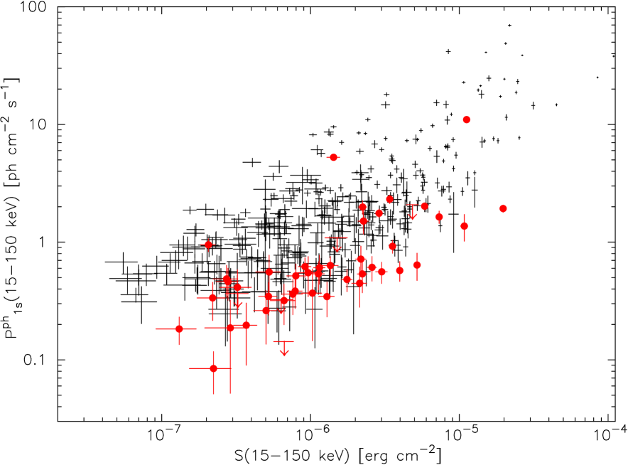
Figure 5.— The 1-s peak photon flux in the 15-150 keV band versus the fluence in the 15-150 keV band for the Swift GRBs in the BAT2 catalog (Sakamoto et al., 2010) overlaid with 64s image triggered GRBs (red).

There are some other reasons for focusing on the image triggered bursts to obtain a reasonable detection threshold of BAT. Figure 5 shows a diagram of the peak photon fluxes and the fluences in the $15-150\;$keV band of Swift GRBs in the BAT2 catalog which includes $64\;$s image triggered GRBs (Sakamoto et al., 2010). The BAT GRBs found by the 64 s image trigger have systematically weaker peak photon flux (but similar fluence) compared to those GRBs found by the rate triggers. Furthermore, the prompt emission and external shock emission of Pop. III GRBs are likely to have a lower peak flux and a longer duration, and to be less variable due to intrinsic property and high-redshift time stretching. The image trigger mode may be more sensitive to such emission than the rate trigger mode. Indeed, the high-redshift GRB 050904 (with $z\simeq 6.3$, Kawai et al., 2006) and the low-luminosity GRB 060218 (Campana et al., 2006; Toma et al., 2007) were image triggered bursts. Thus the estimate of the threshold of the image trigger mode may be relevant especially for Pop. III GRBs. (Note, however, that GRB 090423 (with $z\simeq 8.2$, Tanvir et al., 2009; Salvaterra et al., 2009) and GRB 080913 (with $z\simeq 6.7$, Greiner et al., 2009) are the rate triggered bursts.)

There are 72 GRBs (out of 467 GRBs) detected by the image trigger in the 2nd BAT GRB catalog. Out of 72 imaged triggered GRBs, there are 50 GRBs found by the image trigger with an integration time of $64\;$s, which have been shown in the red points in Figure 5. We focus on this sample of 50 GRBs to estimate the BAT detection threshold. To understand the BAT detection threshold for the image trigger GRBs, we create the spectrum using the $64\;$s image trigger interval, and extract the photon fluence of the interval in the $15-50\;$keV band (same energy band of the image trigger) and the best fit photon index based on a simple power-law model. The image trigger interval has a duration of 64 s starting from the BAT trigger time. Figure 6 shows the distribution of the photon index and the photon fluence in the $15-50\;$keV band for a 64 s image interval of 50 image trigger GRBs. The imaged fluence in the $15-50\;$keV band does not have a strong dependence on the observed spectrum. Therefore, we conclude that the photon fluence threshold of the BAT $64\;$s image trigger is $\sim 1\;{\rm ph}\;{\rm cm}^{-2}$ in the $15-50\;$keV band, corresponding to a photon fluence threshold in the $15-150\;$keV band, of $\sim 2\;{\rm ph}\;{\rm cm}^{-2}$. This corresponds to the averaged photon flux $\sim 0.03\;{\rm ph}\;{\rm cm}^{-2}\;{\rm s}^{-1}$ in the $15-150\;$keV band. Note that this is the minimum averaged flux in the first $64\;$s interval of the image triggered GRBs, which is different from their minimum peak flux for the total observed duration, shown in Figure 5.

Figure 6.— The photon index versus the photon fluence in the 15-50 keV band in the image interval of the 64s image triggered GRBs. The spectral model is a simple power-law model.

Table 1Prompt emission parameters for 33 image trigger GRBs with no optical counterpart. $T_{90}$ is $T_{90}$ duration of the burst. S(15-150) is the fluence in the 15-150 keV band. P${}^{1s}_{\rm ph}$(15-150) is the 1-s peak photon flux in the 15-150 keV band. F^IT(15-50) is the energy flux measured in the image triggered 64 s interval in the 15-50 keV band. PL PhIndex^IT is the photon index based on a simple power-law model to the spectrum of the 64 s image triggered interval.

GRB	$T_{90}$	S(15-150)	P${}^{1s}_{\rm ph}$(15-150)	FIT(15-50)	PL PhIndexIT
	(s)	(erg cm-2)	(ph cm-2 s-1)	(erg cm-2 s-1)
050714B	46.9	$(5.3\pm 1.0)\times 10^{-7}$	$0.6\pm 0.2$	$(6.0\pm 1.0)\times 10^{-9}$	$2.5\pm 0.4$
050803	88.1	$(2.2\pm 0.1)\times 10^{-6}$	$1.0\pm 0.1$	$(4.2\pm 0.8)\times 10^{-9}$	$1.6\pm 0.3$
050916	80.0	$(1.1\pm 0.2)\times 10^{-6}$	$0.5\pm 0.2$	$(4.3\pm 0.7)\times 10^{-9}$	$1.8\pm 0.3$
050922B	156.3	$(2.4\pm 0.4)\times 10^{-6}$	$1.1\pm 0.4$	$(7.2\pm 1.0)\times 10^{-9}$	$2.0\pm 0.3$
051001	190.6	$(1.8\pm 0.1)\times 10^{-6}$	$0.5\pm 0.1$	$(2.6\pm 0.6)\times 10^{-9}$	$2.0\pm 0.3$
051213	71.1	$(8.0\pm 1.0)\times 10^{-7}$	$0.5\pm 0.1$	$(3.4\pm 0.6)\times 10^{-9}$	$1.6\pm 0.3$
051221B	39.9	$(9.1\pm 1.0)\times 10^{-7}$	$0.6\pm 0.2$	$(2.4\pm 0.5)\times 10^{-9}$	$1.7\pm 0.3$
060211A	118.2	$(1.6\pm 0.1)\times 10^{-6}$	$0.4\pm 0.1$	$(3.0\pm 0.3)\times 10^{-9}$	$1.4\pm 0.2$
060319	8.9	$(2.4\pm 0.3)\times 10^{-7}$	$1.1\pm 0.1$	$(2.3\pm 0.4)\times 10^{-9}$	$2.0\pm 0.4$
060413	117.3	$(3.6\pm 0.1)\times 10^{-6}$	$0.9\pm 0.1$	$(2.3\pm 0.5)\times 10^{-9}$	$1.6\pm 0.3$
060427	62.0	$(5.0\pm 0.9)\times 10^{-7}$	$0.3\pm 0.1$	$(3.1\pm 0.5)\times 10^{-9}$	$2.0\pm 0.4$
060516	161.2	$(1.0\pm 0.2)\times 10^{-6}$	$0.4\pm 0.2$	$(3.4\pm 0.6)\times 10^{-9}$	$2.0\pm 0.3$
060728†	-	$(2.2\pm 0.7)\times 10^{-7}$	$0.08\pm 0.02$	$(1.2\pm 0.4)\times 10^{-9}$	$1.4\pm 0.4$
060923C	67.4	$(1.6\pm 0.2)\times 10^{-6}$	$0.9\pm 0.3$	$(1.1\pm 0.1)\times 10^{-8}$	$2.2\pm 0.2$
061027†	-	$(2.9\pm 0.9)\times 10^{-7}$	$0.2\pm 0.1$	$(2.2\pm 0.7)\times 10^{-9}$	$1.9\pm 0.5$
061028	105.6	$(9.5\pm 1.7)\times 10^{-7}$	$0.6\pm 0.2$	$(3.0\pm 0.6)\times 10^{-9}$	$1.9\pm 0.4$
070126†	-	$(1.3\pm 0.4)\times 10^{-7}$	$0.18\pm 0.04$	$(1.2\pm 0.4)\times 10^{-9}$	$1.9\pm 0.5$
070429A	168.0	$(9.4\pm 1.4)\times 10^{-7}$	$0.4\pm 0.1$	$(3.9\pm 0.6)\times 10^{-9}$	$2.2\pm 0.3$
070520A	71.0	$(5.0\pm 1.0)\times 10^{-7}$	$0.3\pm 0.1$	$(2.5\pm 0.5)\times 10^{-9}$	$1.9\pm 0.3$
070704	377.6	$(5.9\pm 0.3)\times 10^{-6}$	$2.0\pm 0.1$	$(1.1\pm 0.1)\times 10^{-8}$	$2.2\pm 0.2$
070920A	51.5	$(5.2\pm 0.7)\times 10^{-7}$	$0.3\pm 0.1$	$(2.9\pm 0.4)\times 10^{-9}$	$1.6\pm 0.2$
071018⋆	288.0	$(1.1\pm 0.2)\times 10^{-6}$	$<0.2$	$(1.0\pm 0.2)\times 10^{-9}$	$1.6\pm 0.3$
071021	228.7	$(1.4\pm 0.2)\times 10^{-6}$	$0.6\pm 0.1$	$(2.6\pm 0.5)\times 10^{-9}$	$1.8\pm 0.4$
071028A⋆	33.0	$(3.3\pm 0.6)\times 10^{-7}$	$<0.4$	$(3.0\pm 0.5)\times 10^{-9}$	$1.8\pm 0.2$
080207‡	$>290$	-	-	$(6.7\pm 0.5)\times 10^{-9}$	$1.3\pm 0.1$
080325⋆	162.8	$(4.9\pm 0.4)\times 10^{-6}$	$<2.0$	$(1.4\pm 0.3)\times 10^{-8}$	$1.5\pm 0.3$
081017⋆	$>320$	$(1.4\pm 0.2)\times 10^{-6}$	$0.2\pm 0.1$	$(1.9\pm 0.3)\times 10^{-9}$	$1.6\pm 0.2$
081022	157.6	$(2.6\pm 0.2)\times 10^{-6}$	$0.6\pm 0.1$	$(7.5\pm 0.6)\times 10^{-9}$	$1.4\pm 0.1$
090308	25.1	$(2.2\pm 0.5)\times 10^{-7}$	$0.3\pm 0.1$	$(3.1\pm 0.5)\times 10^{-9}$	$2.4\pm 0.4$
090401A	117.0	$(1.12\pm 0.03)\times 10^{-5}$	$11.0\pm 0.4$	$(6.3\pm 0.9)\times 10^{-9}$	$1.6\pm 0.2$
090419⋆	460.7	$(2.7\pm 0.3)\times 10^{-6}$	-	$(3.3\pm 0.5)\times 10^{-9}$	$1.3\pm 0.2$
090807A	146.4	$(2.2\pm 0.2)\times 10^{-6}$	$0.7\pm 0.2$	$(8.6\pm 0.9)\times 10^{-9}$	$2.1\pm 0.2$
091104	107.1	$(7.6\pm 1.2)\times 10^{-7}$	$0.4\pm 0.1$	$(3.0\pm 0.5)\times 10^{-9}$	$1.7\pm 0.3$

We found 33 bursts (out of the 72 image triggered GRBs) with no optical counterpart observed, which are listed in Table 1, by looking through the Gamma-ray bursts Coordinates Network (GCN) circulars. These may be candidates for being high-redshift bursts with $z\gtrsim 6$, and might include Pop. III GRBs. Their $T_{90}$ durations are relatively long, but not as long as the $\sim 1\;$day, predicted for Pop. III GRBs in our model. These $T_{90}$ durations are just the time intervals during which BAT was able to detect 90% of the photons from the sources, which is not necessarily the same as the real duration of the bursts, although it provides a useful uniform measure approximating this quantity. If the burst flux is marginally above the BAT threshold initially and it gradually declines, the $T_{90}$ duration could be much shorter than the real duration.

A bright external shock emission of a Pop. III GRB would trigger the BAT even if the prompt emission flux is below the detection threshold. We calculated the $64\;$s photon fluences of the external shock emission in the $15-50\;$keV band for the cases of Figures 2 and 3 and obtained $S_{\rm ph}\simeq 0.33\;{\rm ph}\;{\rm cm}^{-2}$ and $\simeq 1.5\;{\rm ph}\;{\rm cm}^{-2}$, respectively. The photon fluence in the latter case is marginally above the effective threshold $\sim 1\;{\rm ph}\;{\rm cm}^{-2}$. For the case of $1+z=10$ (Figure 4), we obtained $S_{\rm ph}\simeq 2.0\;{\rm ph}\;{\rm cm}^{-2}$ for the negligible pair production case and $S_{\rm ph}\simeq 7.5\;{\rm ph}\;{\rm cm}^{-2}$ for the significant pair production case. These indicate that BAT will be triggered by the external shock emission in some cases. We have a rough relation $S_{\rm ph}\propto\epsilon_{e}L_{\rm iso}f(p)d_{L}^{-2}$ (see the end of Section 3.3). When the progenitor mass is smaller, leading to $L_{\rm iso}$ three times smaller than the case of Figure 2, the external shock emission for the case of $\epsilon_{e,-1}\simeq f(p)\simeq 1$ and $1+z\gtrsim 10$ will not trigger BAT (where the pair production is negligible for $n_{0}<10^{4}$). In the next section, we use a specific model of the Pop. III GRB prompt emission to examine their detectability.

4.2. Prompt photospheric emission

Pop. III GRB jets are likely to be dominated by Poynting-flux, as discussed in Section 2. The prompt emission mechanism of Poynting-dominated GRB jets (as opposed to the afterglow, on which we concentrated thus far) has been actively discussed in the literature (e.g., Thompson, 1994; Mészáros & Rees, 1997b; Spruit et al., 2001; Lyutikov, 2006). The jet may have a subdominant thermal energy component of electron-positron pairs and photons, so that the emission from the photosphere can be bright. In addition to this, above the photosphere, the magnetic field could be directly converted into radiation via magnetic reconnection or the field energy could be converted into particle kinetic energy which can produce non-thermal radiation via shocks. The existence of the latter emission components is uncertain and they are currently difficult to model. Thus, for simplicity we focus on the photospheric emission, which is essentially unavoidable. Such photospheric emission models of the prompt emission are viable also for baryonic jets, which could work for Pop. I/II GRBs (e.g., Mészáros & Rees, 2000; Rees & Mészáros, 2005; Ioka et al., 2007; Toma et al., 2010). MR10 developed the Poynting-dominated jet model of Mészáros & Rees (1997b) for a Pop. III GRB jet, and estimated the luminosity and temperature of the photospheric emission. Here we recalculate this emission component, taking into account the collimation of the outflow.

Let us assume for simplicity that the opening angle of the jet is roughly constant from the base of the jet, $r_{l}=2g_{h}R_{h}\simeq 9.4\times 10^{7}\;g_{h}M_{h,2.5}\;$cm where $g_{h}$ is a numerical factor, out to the external shock region. The isotropic-equivalent luminosity of the jet is given by $L_{\rm iso}=L_{\rm BZ}(2/\theta_{j}^{2})\simeq 4.4\times 10^{53}\;(a_{h}^{2}/\alpha_{-1}\beta_{1})M_{d,2.5}t_{d,4}^{-1}\theta_{j,-1}^{-2}\;{\rm erg}\;{\rm s}^{-1}$. Denoting by $\sigma$ the ratio of the Poynting energy flux and the particle energy flux at the base, the comoving temperature of the flow is estimated as $T^{\prime}_{l}=(L_{\rm iso}/[(1+\sigma)4\pi r_{l}^{2}ca\Gamma_{l}^{2}])^{1/4}\simeq 5.3\times 10^{5}\;[(1+\sigma)/10]^{-1/4}L_{53.6}^{1/4}r_{l,8}^{-1/2}\Gamma_{l}^{-1/2}\;{\rm eV}/k$, where $L_{53.6}=L_{\rm iso}/10^{53.6}\;{\rm erg}\;{\rm s}^{-1}$, $r_{l,8}=r_{l}/10^{8}\;{\rm cm}$, and $\Gamma_{l}$ is the bulk Lorentz factor of the flow at the base. The dynamics of the flow while it is optically thick is governed by energy conservation ($L_{\rm iso}={\rm const.}$), entropy conservation ($r^{2}{T^{\prime}}^{3}\Gamma={\rm const.}$), and the MHD condition for the flow velocity to be close to the light speed (the lab-frame field strength $B\propto r^{-1}$). The last condition indicates that the Poynting energy is conserved, and so the particle energy is also conserved, i.e., $r^{2}{T^{\prime}}^{4}\Gamma^{2}={\rm const.}$ and $\sigma={\rm const.}$ Then we have $T^{\prime}\propto r^{-1}$ and $\Gamma\propto r$. At the photosphere radius $r=r_{a}$ where the electron-positron pairs recombine, the temperature is given by $kT^{\prime}_{a}\sim 17\;$keV. This leads to

$$r_{a} \simeq 3.1\times 10^{9}\;[(1+\sigma)/10]^{-1/4}L_{53.6}^{1/4}r_{l,8}^{1/2}\Gamma_{l}^{-1/2}\;{\rm cm},$$ (12)

$$\Gamma_{a} \simeq 31\;[(1+\sigma)/10]^{-1/4}L_{53.6}^{1/4}r_{l,8}^{-1/2}\Gamma_{l}^{1/2}.$$ (13)

The observed temperature and the bolometric energy flux of the photospheric emission are then

$$kT_{a} \simeq \frac{\Gamma_{a}kT^{\prime}_{a}}{1+z}$$ (14)

$$\simeq 26\;[(1+\sigma)/10]^{-1/4}L_{53.6}^{1/4}r_{l,8}^{-1/2}\Gamma_{l}^{1/2}[(1+z)/20]^{-1}\;{\rm keV},$$

$$F_{a} \simeq \frac{L_{\rm iso}/(1+\sigma)}{4\pi d_{L}^{2}}$$ (15)

$$\simeq 7.1\times 10^{-9}\;[(1+\sigma)/10]^{-1}L_{53.6}d_{L,20}^{-2}\;{\rm erg}\;{\rm cm}^{-2}\;{\rm s}^{-1}.$$

The photospheric photons can be scattered by MHD turbulence or Alfvén waves, induced by e.g., the interaction of the jet with the stellar envelope, into a power-law spectrum extending up to comoving photon energies $\sim m_{e}c^{2}$ (Thompson, 1994). The emission from the photosphere of Pop. III GRB would thus have a black-body peak, and may have a non-thermal tail extending (in the observer frame) to photon energies $\varepsilon\sim\Gamma_{a}m_{e}c^{2}/(1+z)\sim 1\;$MeV. This photospheric emission may be detected until $t_{\rm obs}=t_{d,{\rm obs}}$. We plot this in Figures 2, 3, and 4 with dotted lines for the case of $1+\sigma=10$ and $L_{53.6}=r_{l,8}=\Gamma_{l}=1$.

We calculated the photon fluences in $64\;$s in the $15-50\;$keV band for the above parameter sets as $S_{\rm ph}\simeq 1.4\;{\rm ph}\;{\rm cm}^{-2}$ for the case of $1+z=20$ and $\simeq 1.3\;{\rm ph}\;{\rm cm}^{-2}$ for the case of $1+z=10$. Thus this emission can be marginally detected by the image trigger of BAT. The value of $\sigma$ is highly uncertain, similar to $R_{*}$ and $\theta_{j}$ for a specific value of $M_{*}$. For $L_{\rm iso}/(1+\sigma)$ three times smaller than the above case (and similar values of $r_{l}$ and $\Gamma_{l}$), the photon fluence is calculated as $<1\;{\rm ph}\;{\rm cm}^{-2}$ both for $1+z=20$ and $1+z=10$, and thus BAT is not expected to be triggered.

4.3. Pop. III GRB Rate

The Pop. III GRB rate is largely uncertain, and has only been inferred from theoretical models. The observed rate of Pop. III GRBs originating between redshifts $z$ and $z+dz$ is computed by

$$\frac{d\dot{N}_{\rm GRB}^{\rm obs}}{dz}=\psi_{*}(z)\eta_{\rm GRB}(z)P(z)\frac{1}{1+z}\frac{dV}{dz}$$ (16)

where $\psi_{*}(z)$ is the Pop. III star formation rate (SFR) per unit comoving volume, $\eta_{\rm GRB}(z)$ is the efficiency of the GRB formation, $P(z)$ is the detection efficiency, i.e., the ratio of the Pop. III GRBs which would be detected by a specific instrument out of the entire number of Pop. III GRBs, and $dV/dz$ is the comoving volume element of the observed area per unit redshift. The additional factor $1/(1+z)$ represents the cosmological time dilation effect.

The factors $\psi_{*}(z)$ and $\eta_{\rm GRB}(z)$ are both highly uncertain for the Pop. III VMSs as well as for the Pop. I/II stars. Just for a concrete discussion, here we use $\psi_{*}(z)$ predicted by using the extended Press-Schechter formalism and the current observational results on the SFR for $z\lesssim 6$ (Bromm & Loeb, 2006) (see also Naoz & Bromberg, 2007). For Pop. I/II stars, they assumed a $z$-independent $\eta_{\rm GRB}\simeq 2\times 10^{-9}\;M_{\odot}^{-1}$ to set the total Pop. I/II GRB rate observed by Swift BAT to be $\sim 90\;{\rm yr}^{-1}$. (Note that they assumed that Swift BAT covers $4\pi$ of the sky, while it actually covers only $\sim 2\pi/3$ of the sky. Thus the GRB formation efficiency should be normalized as $\sim 6$ times their adopted value, $\eta_{\rm GRB}\simeq 1.2\times 10^{-8}\;M_{\odot}^{-1}$.) Their result predicts the Pop. I/II GRB rate observed by BAT at $z>6$ to be $\sim 10\;{\rm yr}^{-1}$. Since a small fraction $\sim 25\%$ of GRBs detected by BAT have redshifts determined, because of bad conditions for optical and near-IR observations (cf. Fynbo et al., 2009, see also our implication from the image triggered GRBs in Section 4.1 and in Table 1), the predicted rate of Pop. I/II GRBs with $z$ determined would be $\sim 3\;{\rm yr}^{-1}$. This is somewhat higher than the current observed rate, $0.6\;{\rm yr}^{-1}$, i.e., 3 GRBs (GRB 050904, GRB 080913, and GRB 090423) during the 5-yr operation of Swift, but their model of $\psi_{*}(z)$ and $\eta_{\rm GRB}$ is not interpreted as unacceptable, taking into account the uncertainties of the theoretical calculations and the poor statistics of the current observed data. For Pop. III stars, they assumed the same $z$-independent $\eta_{\rm GRB}$ as Pop. I/II stars and computed the nominal Pop. III GRB rate observed by BAT to be $R_{\rm BAT}\approx zd\dot{N}_{\rm GRB}^{\rm obs}/dz\sim 0.03\;{\rm yr}^{-1}$ for bursts around $z\sim 20$ and $\sim 0.3\;{\rm yr}^{-1}$ for bursts around $z\sim 10$.

The detection efficiency $P(z)$ is computed by assuming the GRB luminosity function and the detection threshold. Bromm & Loeb (2006) assumed that the Pop. III GRB luminosity function is the same as that of Pop. I/II GRBs and took a BAT detection threshold of $f_{\rm ph,lim}\simeq 0.2\;{\rm ph}\;{\rm cm}^{-2}\;{\rm s}^{-1}$. We can assume, however, that the Pop. III GRBs have a different luminosity function, with a brighter membership than Pop. I/II GRBs, and take the effective BAT threshold deduced by our analysis of the image trigger bursts (see Section 4.1), in which case $R_{\rm BAT}$ can be larger than the above estimate.

In order to estimate $R_{\rm BAT}$ in our Pop. III GRB model, let us first presume the observed rate (for $\sim 2\pi/3$ of the sky) if we would detect the entirety of the Pop. III GRBs originating around $z\sim 10-20$ without considering the detection efficiency, $R_{w}$, based on the calculations of Bromm & Loeb (2006). The detection efficiency is computed by

$$P(z)=\int^{\infty}_{L_{\rm ph,lim}(z)}p(L_{\rm ph})dL_{\rm ph},$$ (17)

where $L_{\rm ph}$ is the isotropic-equivalent photon luminosity of a burst, and $p(L_{\rm ph})$ is the luminosity function normalized as $\int^{\infty}_{0}p(L_{\rm ph})dL_{\rm ph}=1$. They adopted $L_{\rm ph,lim}=4\pi d_{L}^{2}f_{\rm ph,lim}\simeq 1\times 10^{60}\;{\rm ph}\;{\rm s}^{-1}$ for bursts around $z\sim 20$ and $\simeq 2\times 10^{59}\;{\rm ph}\;{\rm s}^{-1}$ for bursts around $z\sim 10$. The detection efficiency is then roughly estimated to be $\sim p(L_{\rm ph,lim})L_{\rm ph,lim}/p(L_{p})L_{p}\sim 0.2$ for $z\sim 20$ and $\sim 0.5$ for $z\sim 10$, where $L_{p}$ provides the peak of the function of $p(L_{\rm ph})L_{\rm ph}$. Thus, we obtain $R_{w}\sim R_{\rm BAT}/0.2\sim 0.2\;{\rm yr}^{-1}$ for $z\sim 20$ and $\sim R_{\rm BAT}/0.5\sim 0.6\;{\rm yr}^{-1}$ for $z\sim 10$.

According to our study in Sections 4.1 and 4.2, the photospheric prompt emission and/or the external shock emission of Pop. III GRBs can be detected by the BAT image trigger for our fiducial set of parameters, $M_{d,2.5}\simeq M_{h,2.5}\simeq R_{*,12}\simeq\theta_{j,-1}\simeq\epsilon_{e,-1}\simeq f(p)\simeq(1+\sigma)/10\simeq 1$ and $1+z\gtrsim 10$, while not detected for $L_{\rm iso}$ just three times smaller than that for the above set of parameters. Thus, if the distribution of the parameters of the Pop. III VMSs clusters around our fiducial set of parameters, BAT would detect, say, about half of the Pop. III GRBs out of the whole Pop. III GRBs, i.e., the detection rate could be $R_{\rm BAT}\sim R_{w}/2\sim 0.1\;{\rm yr}^{-1}$ for $z\sim 20$ and $\sim 0.3\;{\rm yr}^{-1}$ for $z\sim 10$. These values have large uncertainties, but imply that the 5-yr operation of Swift so far may already have detected a Pop. III GRB, or may detect it in the near future, if the factor $\psi_{*}(z)\times\eta_{\rm GRB}$ is given as above.

5. Late-Time Radio Afterglows

We have focused so far on the high-energy emission just before and near the beginning of the external shock self-similar phase ($t_{\rm obs}\simeq t_{d,{\rm obs}}$, see Figure 1) to constrain the physical parameters $E_{\rm iso}$ and $n$ of Pop. III GRBs, and to examine their detectability by BAT. In this section, we argue that the radio afterglows of Pop. III GRBs in the self-similar phase ($t_{\rm obs}>t_{d,{\rm obs}}$) can be so bright that they also provide powerful tools for constraining the event rate. At $t_{d,{\rm obs}}$, the flux of the external shock emission shown in Figure 2 at $\nu_{a}\simeq 230\;E_{57.6}^{1/6}t_{d,4}^{-1/2}n_{0}^{1/6}[(1+Y)/3.7]^{-1/3}[(1+z)/20]^{-1}\;$GHz is given by

$$F_{\nu_{a}}\simeq 2.6\;\epsilon_{B,-2}^{-1/4}E_{57.6}^{2/3}n_{0}^{-1/12}[(1+Y)/3.7]^{-5/6}[(1+z)/20]d_{L,20}^{-2}\;{\rm Jy}.$$ (18)

The break frequency $\nu_{a}$ decreases (as $t_{\rm obs}^{-1/2}$) but the flux at $\nu_{a}$ stays constant after $t_{d,{\rm obs}}$, at least until the epoch when the jet effects become significant. This indicates that the Pop. III GRB afterglows can be very bright radio sources, despite their large distances.

We briefly compute the light curves at various frequencies in the radio bands, 100 GHz, 5 GHz, 1 GHz, and 70 MHz, in our fiducial case, $E_{57.6}=t_{d,4}=n_{0}=\epsilon_{B,-2}=\epsilon_{e,-1}=f(p)=\theta_{j,-1}=1$. As discussed above, the temporal evolution of the characteristic quantities of the external shock in the self-similar expansion phase can be obtained by replacing $t_{d}$ by the variable $t_{\rm obs}$ and taking the other parameters as constant in the equations of the general afterglow model (shown in Appendix). The jet effects are significant when the Lorentz factor of the shocked fluid is $\Gamma\simeq\theta_{j}^{-1}$, i.e., at the observer’s time

$$t_{\theta,{\rm obs}}\simeq\left(\frac{E_{\rm iso}\theta_{j}^{8}}{4\pi nm_{p}c^{5}}\right)^{1/3}(1+z)\simeq 9.9\times 10^{2}\;E_{57.6}^{1/3}n_{0}^{-1/3}\theta_{j,-1}^{8/3}[(1+z)/20]\;{\rm day}.$$ (19)

After $t_{\theta,{\rm obs}}$, the temporal evolution of the characteristic quantities is obtained by replacing $E_{\rm iso}$ by $t_{\rm obs}^{-1}$ and $t_{d}$ by $t_{\rm obs}$, respectively, and taking the other parameters as constant (Sari et al., 1999). Such an evolution is derived under the assumption that the shocked fluid expands sideways rapidly after $t_{\theta,{\rm obs}}$. Recent detailed hydrodynamic simulations (Zhang & MacFadyen, 2009; Granot, 2007) have shown that the shocked fluid only undergoes a slow sideways expansion, while the afterglow light curves can be still approximated by those predicted by Sari et al. (1999) especially in the radio band. (In the optical and X-ray bands, the spectrum is so soft that the limb-brightening effect is significant. Then the brightest portion at an angle $\theta\sim\Gamma^{-1}$ from the line of sight becomes missing at $t_{\theta,{\rm obs}}$, which causes a steeper light curve than $t_{\rm obs}^{-p}$.)

In an analytical treatment (e.g., Sari et al., 1999) the rapid sideways expansion of the fluid would lead to a nearly spherical ($\theta_{j}\sim 1$) configuration of the shocked fluid leading to the non-relativistic Sedov-von Neumann-Taylor (SNT) solution, starting around observer’s time $t_{\rm SNT,obs}\simeq[E_{\rm iso}\theta_{j}^{2}/(4\pi nm_{p}c^{5})]^{1/3}(1+z)\simeq 9.9\times 10^{4}\;E_{57.6}^{1/3}n_{0}^{-1/3}\theta_{j,-1}^{2/3}[(1+z)/20]\;$day. However, the detailed hydrodynamic simulations (Zhang & MacFadyen, 2009) show that the much slower sideways expansion results in the later start of the SNT phase. The starting time is shown to be a few times $t_{\rm NR,obs}$

$$t_{\rm NR,obs}\simeq\left(\frac{E_{\rm iso}}{4\pi nm_{p}c^{5}}\right)^{1/3}(1+z)\simeq 4.6\times 10^{5}\;E_{57.6}^{1/3}n_{0}^{-1/3}[(1+z)/20]\;{\rm day},$$ (20)

where the shocked fluid is still highly collimated. The temporal evolution of the characteristic quantities in the SNT phase is obtained by using $r\propto t_{\rm obs}^{2/5}$ and $v\propto t_{\rm obs}^{-3/5}$, where $v$ is the velocity of the shocked fluid, and the internal energy density is $\propto v^{2}$. This results in a light curve with a shallower decay at $\nu>\nu_{a}$ (or a steeper rise at $\nu<\nu_{a}$) in the SNT phase, compared to the decay in the prior phase. Therefore, the assumption of the slow sideways expansion and the late SNT phase based on the numerical simulations leads to smaller number of off-axis observers (due to the high collimation) and dimmer radio fluxes than that of the rapid sideways expansion based on the approximate analytical arguments. We here take the former, conservative assumption of the slow sideways expansion.

Figure 7.— Radio light curves at frequencies, 100 GHz (dot-dashed line), 5 GHz (dotted line), 1 GHz (solid line), and 70 MHz (dashed line), of a Pop. III GRB at $1+z=20$ with typical parameters $E_{57.6}=t_{d,4}=n_{0}=\epsilon_{B,-2}=\epsilon_{e,-1}=f(p)=\theta_{j,-1}=1$. The important observer’s times are the jet duration $t_{d,{\rm obs}}\simeq 2.3\;$day, the jet break time $t_{\theta,{\rm obs}}\simeq 9.9\times 10^{2}\;$day, and the time when the shock becomes non-relativistic $t_{\rm NR,obs}\simeq 4.6\times 10^{5}\;$day.

For calculating the radio emission we need to compute only the synchrotron emission of the original electrons. At late times, the number of pairs is typically small, and the pair emission is negligible. The SSC emission is not relevant in the radio bands. The results are plotted in Figure 7. Here we confirmed the assumptions that all the electrons in the shocked region remain relativistic at least until $t_{\rm obs}=10^{6}\;$day.

Figure 7 shows that the radio afterglows of Pop. III GRBs can be very bright with a very long duration. These could have been detected as quasi-steady point sources by the radio survey observations. As far as we know, the current largest radio survey data is based on the Very Large Array (VLA) FIRST survey (White et al., 1997), which observed a large area mainly around the north Galactic cap at 1.4 GHz, covering $\sim 1/5$ of all the sky. For the threshold, $\sim 6\;$mJy at 1.4 GHz, a Pop. III GRB radio afterglow at $1+z=20$ (at $1+z=10$) can be observed for $t_{rd,{\rm obs}}\sim 300\;$yr (for $t_{rd,{\rm obs}}\sim 200\;$yr). Therefore, if we denote by $R_{w,4\pi}$ the all-sky Pop. III GRB rate in unit of ${\rm yr}^{-1}$, the number of the Pop. III radio afterglows that would have been detected in that survey is estimated to be $\sim(R_{w,4\pi}/5)t_{rd,{\rm obs}}\sim 60\;(R_{w,4\pi}/1\;{\rm yr}^{-1})(t_{rd,{\rm obs}}/300\;{\rm yr})$ for bursts at $1+z\sim 20$, and $\sim 200\;(R_{w,4\pi}/4\;{\rm yr}^{-1})(t_{rd,{\rm obs}}/200\;{\rm yr})$ for bursts at $1+z\sim 10$. A detailed analysis of the FIRST data would thus provide a powerful constraint on $R_{w,4\pi}$ of Pop. III GRBs such as discussed in this paper (even no sources like our model calculations would provide an upper limit on the rate). The Pop. III radio sources could have X-ray counterparts. In our model the late time X-ray afterglow is dominated by the SSC component, whose flux in the $0.3-10\;$keV range can be $>10^{-15}\;{\rm erg}\;{\rm cm}^{-2}\;{\rm s}^{-1}$ for $t_{\rm obs}\lesssim 100\;$yr (which can be detected by Chandra X-ray Observatory).

The above predicted numbers of the Pop. III GRB radio afterglows are just based on the values of $t_{rd,{\rm obs}}$ calculated for our fiducial set of parameters. In order to obtain more realistic numbers taking into account the distributions of the model parameters, we require to calculate the radio light curves for large ranges of parameter values. However, the radio light curves may highly depend on the parameters $E_{\rm iso},t_{d},n,\epsilon_{B},\epsilon_{e}$, and $f(p)$. In other words, there are many patterns of light curves depending on the orders of characteristic times $t_{a=c},t_{m=a},$ and $t_{m=c}$, which are the times when $\nu_{a}$ crosses $\nu_{c}$, when $\nu_{m}$ crosses $\nu_{a}$, and $\nu_{m}$ crosses $\nu_{c}$, respectively, as well as $t_{d},t_{\theta},$ and $t_{\rm NR}$ (we have $t_{d}<t_{\theta}<t_{m=a}<t_{m=c}<t_{a=c}<t_{\rm NR}$ for our adopted parameter set). A thorough model analysis with different parameter sets would deserve another future work.

Recent radio transient searches without primary detections at any other frequencies have begun to open new observational frontiers (e.g., Niinuma et al., 2007; Bower et al., 2007; Ofek et al., 2010), but currently they do not appear to have good potentials for detecting Pop. III GRB radio afterglows. The interferometric drift-scanning observation with the Waseda Nasu Pulsar Observatory in Japan may scan a large area at $1.4\;$GHz (Niinuma et al., 2007), but its detection thereshold, $\sim 0.3\;$Jy, is not sufficiently high for searching our typical Pop. III radio afterglows. Bower et al. (2007) reported results of a survey for transient sources by using archival data obtained with VLA observation of a single field at 5 or 8.4 GHz, but the field is very small, $<0.1\;{\rm deg}^{2}$.

The absorption line at 21 cm (associated with transitions between the hyperfine levels of the hydrogen atom) seen in the continuum radio spectrum of high-redshift sources would be one of the promising tools to reveal the reionization histroy of the universe (Tozzi et al., 2000; Shaver et al., 1999). GRB radio afterglows have been considered as candidate backlighting sources, but the bursts with the usual or slightly higher total energies have been found to be too dim for this aim (Furlanetto & Loeb, 2002; Ioka & Mészáros, 2005). However, the high-redshift GRBs arising from Pop. III VMSs, such as discussed in this paper, can emit a sufficiently bright radio afterglow to be of interest. For our fiducial parameter values, the radio flux at $\nu=1420\;{\rm MHz}/(1+z)$ is estimated to be $\simeq 2.4\;$mJy (with peak time $t_{p,{\rm obs}}\simeq 850\;$yr) for $1+z=20$ and $\simeq 6.4\;$mJy (with peak time $t_{p,{\rm obs}}\simeq 430\;$yr) for $1+z=10$, which are comparable to the lower bound on the radio flux for detection of the 21 cm absorption line, $\sim 1-10\;$mJy (Ioka & Mészáros, 2005). Thus the 21 cm absorption line could be marginally detected in the Pop. III GRB radio afterglows. A radio survey with telescopes like Low Frequency Array (LOFAR) could detect such radio afterglows and determine their redshifts by their 21 cm lines themselves. The predicted number of detections is $\sim R_{w,4\pi}(\Omega/4\pi)t_{p,{\rm obs}}\sim 1\;(R_{w,4\pi}/1\;{\rm yr}^{-1})(\Omega/50\;{\rm deg}^{2})(t_{p,{\rm obs}}/850\;{\rm yr})$ for bursts at $1+z\sim 20$, and $\sim 1\;(R_{w,4\pi}/4\;{\rm yr}^{-1})(\Omega/20\;{\rm deg}^{2})(t_{p,{\rm obs}}/430\;{\rm yr})$ for bursts at $1+z\sim 10$, where $\Omega$ is the solid angle of the survey area. Note that the jets will keep collimated even around $\sim t_{\rm NR,obs}$ due to the slow sideways expansions (Zhang & MacFadyen, 2009), so that off-axis viewings of the afterglows are too dim to detect.

6. Summary

Pop. III GRBs may have an isotropic-equivalent energy $E_{\rm iso}\gtrsim 10^{57}\;$erg and a cosmological-rest-frame duration $t_{d}\gtrsim 10^{4}\;$s. We have calculated the external shock emission spectrum at $t_{d,{\rm obs}}$ in detail based on the standard model (Mészáros & Rees, 1997a; Sari et al., 1998; Sari & Esin, 2001; Nakar et al., 2009). This model can explain many of the X-ray/optical/radio afterglows detected so far (e.g., Panaitescu & Kumar, 2002; Liang et al., 2007) as well as the very early high-energy afterglows detected by Fermi LAT (e.g., Kumar & Barniol Duran, 2009; De Pasquale et al., 2010; Corsi et al., 2010).

We found that the external shock emission at $t_{d,{\rm obs}}$ can be detected by Fermi LAT and Swift XRT/BAT, whose flux leads to a constraint on $E_{\rm iso}$ by using the source redshift (and distance) that will be determined by the observation of the Ly$\alpha$ drop-off in the IR band. The detection of a burst at $z\gtrsim 10$ with $E_{\rm iso}\gtrsim 10^{57}\;$erg and $t_{d}\gtrsim 10^{4}\;$s would be a very strong indication that this is a GRB arising from a Pop. III VMS with $M_{*}\gtrsim 300\;M_{\odot}$. This indication should be complemented with the constraint on the metal abundances in the surrounding medium through high resolution IR and X-ray spectroscopy.

One of the important findings of the present study is that the $\gamma\gamma$ self-absorption break at energy $\varepsilon_{\gamma\gamma}$ in some cases of the external shock emission spectrum of a Pop. III GRB is expected to be observable in the LAT energy range. Given that the prompt emission at $t_{d,{\rm obs}}$ does not hide the external shock emission in the LAT range and $\varepsilon_{\gamma\gamma}$ is well below the values of the EBL $\gamma\gamma$ cutoff energy expected for practically all EBL models with the determined source redshift, we have shown that the flux and the energy $\varepsilon_{\gamma\gamma}$, together with Swift XRT data, can lead to a constraint on the value of the external density $n$. The constraint on $n$ would provide invaluable information about the environment and the radiative feedback processes of Pop. III stars.

Putting constraints on $n$ from the $\gamma\gamma$ self-absorption break is a fairly new method, while constraints on $n$ from the multi-wavelength observations of the late-time afterglows of Pop. I GRBs are common (e.g., Panaitescu & Kumar, 2002; Wijers & Galama, 1999). Here we have discussed the conditions under which these methods can be used in Pop. III GRBs. One caveat is that we have assumed that the electron acceleration processes works uniformly in the emitting region for calculating the afterglow spectra. As discussed below Equation (A19) in Appendix, it is also possible that the electron acceleration works only near the shock front, where $\varepsilon_{\gamma\gamma}$ may be far above the LAT energy range, and $\varepsilon_{M}$ depends on the unknown upstream magnetic field strength, which do not allow us to constrain $n$.

In order to identify the direction to GRB afterglows on the sky for observations with Swift, Fermi, and the IR telescopes, the emission needs to be high enough to trigger the large field instrument BAT. A reasonable trigger threshold of Swift BAT can be estimated by focusing on the image trigger mode, since it is based on a criterion with a fixed time-scale and energy band, while more general BAT threshold including the usual rate trigger is too complicated to estimate. The image trigger mode may be suitable for detecting weak and less-variable bursts like very-high-redshift bursts. We have used the samples in the BAT2 catalog and deduced the detection threshold of the BAT image trigger to be $\sim 1\;{\rm ph}\;{\rm cm}^{-2}$ for the $64\;$s interval in the $15-50\;$keV band. We have calculated the prompt photospheric emission flux of Pop. III GRBs with typical parameters, and shown that these can be marginally detected by BAT. The external shock emission can also trigger BAT without the prompt emission trigger in some cases.

We have also briefly shown that the Pop. III GRB late-time radio afterglows can be very bright. For our fiducial parameters, the peak flux at $1\;$GHz is $\simeq 140\;$mJy, which could be identified in the VLA FIRST survey data. This survey covered a sufficiently large area, which would provide a powerful upper bound on the rate of the Pop. III GRBs. The peak flux of the late-time $70\;$MHz radio afterglow for our fiducial parameters is $\simeq 2.4\;$mJy, in which 21 cm absorption lines could be detected. This would provide a measure of the neutral hydrogen fraction in the IGM around the Pop. III star.

Putting constraints on the properties of Pop. III stars has recently become of great importance in modern cosmology. Planned IR surveys will be able to probe Pop. III stars. However, it is difficult to distinguish between a single Pop. III VMS and a cluster of less massive Pop. III stars. Thus, the detection of GRBs with very high $E_{\rm iso}$ and very long $t_{d}$ could provide critical, ‘smoking gun’ evidence for the existence of VMSs. Multi-wavelength observations of such GRBs with Swift, Fermi, and ground-based IR and radio telescopes should provide us with invaluable information on Pop. III stars and their environments.

Appendix A General Model

The afterglow emission spectrum at the time $t_{d}$ is determined by the radius $r_{d}$ and the Lorentz factor $\Gamma_{d}$ of the shocked fluid at this time, which are given via the relations $E_{\rm iso}\simeq 4\pi r_{d}^{3}\Gamma_{d}^{2}nm_{p}c^{2}$ and $r_{d}\simeq c\Gamma_{d}^{2}t_{d}$. Here we have assumed for simplicity that the circumburst medium density is uniform, $n=1\;n_{0}\;{\rm cm}^{-3}$. These two equations lead to

$$r_{d} \simeq \left(\frac{E_{\rm iso}t_{d}}{4\pi nm_{p}c}\right)^{1/4}\simeq 2.8\times 10^{18}\;E_{57.6}^{1/4}t_{d,4}^{1/4}n_{0}^{-1/4}\;{\rm cm}$$ (A1)

$$\Gamma_{d} \simeq \left(\frac{E_{\rm iso}}{4\pi nm_{p}c^{5}t_{d}^{3}}\right)^{1/8}\simeq 97\;E_{57.6}^{1/8}t_{d,4}^{-3/8}n_{0}^{-1/8},$$ (A2)

where $E_{57.6}=E_{\rm iso}/10^{57.6}\;{\rm erg}$ and $t_{d,4}=t_{d}/10^{4}\;{\rm s}$. The magnetic field strength in the shocked region scales as

$$B\simeq(32\pi\epsilon_{B}nm_{p}c^{2})^{1/2}\Gamma_{d}\simeq 3.8\;\epsilon_{B,-2}^{1/2}E_{57.6}^{1/8}t_{d,4}^{-3/8}n_{0}^{3/8}\;{\rm G},$$ (A3)

where $\epsilon_{B,-2}=\epsilon_{B}/10^{-2}$. The minimum injected electron Lorentz factor is

$$\gamma_{m}\simeq\epsilon_{e}\Gamma_{d}\frac{m_{p}}{m_{e}}\frac{p-2}{p-1}\simeq 4.1\times 10^{3}\;\epsilon_{e,-1}E_{57.6}^{1/8}t_{d,4}^{-3/8}n_{0}^{-1/8}f(p),$$ (A4)

where $\epsilon_{e,-1}=\epsilon_{e}/10^{-1}$ and $f(p)=(13/3)(p-2)/(p-1)$. We have assumed that all the electrons are accelerated to a power-law spectrum $dn/d\gamma_{e}\propto\gamma_{e}^{-p}$ for $\gamma_{e}\geq\gamma_{m}$.

The accelerated electrons will lead to synchrotron and SSC emission. The radiative cooling timescale in the comoving frame is $t^{\prime}_{c}=6\pi m_{e}c/[\sigma_{T}\gamma_{e}B^{2}(1+Y(\gamma_{c}))]$, where $Y(\gamma_{c})$ is the luminosity ratio of the SSC to synchrotron emission for electrons with $\gamma_{c}$, while the comoving dynamical timescale is $t^{\prime}_{d}=\Gamma_{d}t_{d}$. Thus the electron Lorentz factor above which the radiative cooling is more significant than the adiabatic cooling is

$$\gamma_{c}\simeq\frac{6\pi m_{e}c}{\sigma_{T}B^{2}\Gamma_{d}t_{d}[1+Y(\gamma_{c})]}\simeq 56\;[1+Y(\gamma_{c})]^{-1}\epsilon_{B,-2}^{-1}E_{57.6}^{-3/8}t_{d,4}^{1/8}n_{0}^{-5/8}.$$ (A5)

All the injected electrons are radiatively cooled within the dynamical timescale if $\gamma_{c}<\gamma_{m}$, that is if

$$\epsilon_{B,-2}n_{0}^{1/2}[1+Y(\gamma_{c})]>1.4\times 10^{-2}\;\epsilon_{e,-1}^{-1}E_{57.6}^{-1/2}t_{d,4}^{1/2}{f(p)}^{-1}.$$ (A6)

This condition can be rewritten using Eqs. (3) and (6) as

$$M_{d,2.5}^{1/2}M_{h,2.5}^{1/4}R_{*,12}^{-3/4}n_{0}^{1/2}\theta_{j,-1}^{-1}a_{h}\beta_{1}^{-1/2}(1-\epsilon_{\gamma})^{1/2}>10^{-2}\epsilon_{B,-2}^{-1}\epsilon_{e,-1}^{-1}{f(p)}^{-1}[1+Y(\gamma_{c})]^{-1}.$$ (A7)

Since the masses $M_{d}$ and $M_{h}$ are expected to be positively correlated with the radius $R_{*}$, this condition is found to be satisfied for reasonable parameter ranges. We thus focus on the fast-cooling regime, $\gamma_{c}<\gamma_{m}$ for the emission at $t_{d}$.

The peak energies of the $\varepsilon F_{\varepsilon}$ spectra of the synchrotron and SSC emission are given by

$$\varepsilon_{m} \simeq \frac{3heB}{4\pi m_{e}c}\gamma_{m}^{2}\frac{\Gamma_{d}}{1+z}\simeq 5.4\;\epsilon_{e,-1}^{2}\epsilon_{B,-2}^{1/2}E_{57.6}^{1/2}t_{d,4}^{-3/2}{f(p)}^{2}[(1+z)/20]^{-1}\;{\rm eV},$$ (A8)

$$\varepsilon_{m}^{\rm SC} \simeq 2\gamma_{m}^{2}\varepsilon_{m}\simeq 1.8\times 10^{2}\;\epsilon_{e,-1}^{4}\epsilon_{B,-2}^{1/2}E_{57.6}^{3/4}t_{d,4}^{-9/4}n_{0}^{-1/4}{f(p)}^{4}[(1+z)/20]^{-1}\;{\rm MeV},$$ (A9)

respectively. If $\varepsilon_{m}^{\rm SC}<\Gamma_{d}\gamma_{m}m_{e}c^{2}/(1+z)$, the Klein-Nishina (KN) suppression of the SSC emission is not significant (e.g., Nakar et al., 2009). This condition is rewritten as $\epsilon_{B,-2}<3.2\times 10^{3}\epsilon_{e,-1}^{-6}E_{57.6}^{-1}t_{d,4}^{3}{f(p)}^{-6}$, which is satisfied for reasonable parameter ranges. In the case of negligible KN effects, $Y$ does not depend on $\gamma_{e}$ for $\gamma_{e}\lesssim\gamma_{m}$, which is calculated from

$$Y\simeq\sigma_{T}\frac{r_{d}}{\Gamma_{d}}\int_{\gamma_{c}}^{\infty}d\gamma_{e}\frac{dn}{d\gamma_{e}}\gamma_{e}^{2}\simeq\tau\gamma_{c}\gamma_{m}\frac{p-1}{p-2}\simeq\frac{\epsilon_{e}}{\epsilon_{B}}\frac{1}{1+Y},$$ (A10)

where $\tau=\sigma_{T}r_{d}n$ is the optical depth for the electron scattering. We obtain $Y\approx\sqrt{\epsilon_{e}/\epsilon_{B}}\sim 3\;\epsilon_{e,-1}^{1/2}\epsilon_{B,-2}^{-1/2}$ for the case of $\epsilon_{e}\gtrsim\epsilon_{B}$, while otherwise $Y\approx\epsilon_{e}/\epsilon_{B}<1$. The SSC spectrum above $\varepsilon_{m}^{\rm SC}$ has a softening break at

$$\varepsilon_{\rm KN}\simeq\frac{\Gamma_{d}^{2}m_{e}^{2}c^{4}}{(1+z)^{2}\varepsilon_{m}}\simeq 1.2\;\epsilon_{e,-1}^{-2}\epsilon_{B,-2}^{-1/2}E_{57.6}^{-1/4}t_{d,4}^{3/4}n_{0}^{-1/4}{f(p)}^{-2}[(1+z)/20]^{-1}\;{\rm TeV}.$$ (A11)

The fluxes at $\varepsilon_{m}$ and at $\varepsilon_{m}^{\rm SC}$ are given by

$$\varepsilon_{m}F_{\varepsilon_{m}} \simeq \frac{\epsilon_{e}E_{\rm iso}t_{d}^{-1}}{4\pi d_{L}^{2}}\frac{p-2}{p-1}\frac{1}{1+Y}$$ (A12)

$$\simeq 1.6\times 10^{-9}\;(1+Y)^{-1}\epsilon_{e,-1}E_{57.6}t_{d,4}^{-1}f(p)d_{L,20}^{-2}\;{\rm erg}\;{\rm cm}^{-2}\;{\rm s}^{-1},$$

$$\varepsilon_{m}^{\rm SC}F_{\varepsilon_{m}}^{\rm SC} \simeq Y\varepsilon_{m}F_{\varepsilon_{m}},$$ (A13)

where the luminosity distance $d_{L}$ is normalized by the value for $1+z=20$, $6.7\times 10^{29}\;$cm. In the case of significant KN effects, i.e., $\varepsilon_{m}^{\rm SC}>\Gamma_{d}\gamma_{m}m_{e}c^{2}/(1+z)$, the SSC emission is not important and $Y$ is smaller than the above value (see Nakar et al., 2009, for details).

The maximum energy of the electrons is determined by equating the acceleration timescale and the radiative cooling timescale. If the electron acceleration occurs in the whole region, we may estimate the (comoving) acceleration timescale as $t^{\prime}_{a}=g2\pi\gamma_{e}m_{e}c/(eB)$ where $g$ is a numerical factor. For electrons with maximum Lorentz factor $\gamma_{M}$, the KN effect is typically significant, and $Y(\gamma_{M})<1$. Then we have $\gamma_{M}\simeq[3e/(g\sigma_{T}B)]^{1/2}$, and its characteristic synchrotron energy is

$$\varepsilon_{M} \simeq \frac{3heB}{4\pi m_{e}c}\gamma_{M}^{2}\frac{\Gamma_{d}}{1+z}=\frac{9he^{2}}{4\pi m_{e}c\sigma_{T}g}\frac{\Gamma_{d}}{1+z}$$ (A14)

$$\simeq 1.8\times 10^{2}\;g^{-1}E_{57.6}^{1/8}t_{d,4}^{-3/8}n_{0}^{-1/8}[(1+z)/20]^{-1}\;{\rm MeV}.$$

The energy $\varepsilon_{a}$ below which the synchrotron self-absorption effect is significant can be estimated by equating the synchrotron flux to the blackbody flux of the characteristic electrons in the shocked region, $F_{\varepsilon_{a}}=[(1+z)^{3}/d_{L}^{2}]2\pi m_{e}\gamma_{ch}(\varepsilon_{a}/h)^{2}(r_{d}^{2}/\Gamma_{d})$ (e.g., Mészáros & Rees, 1997a). The Lorentz factor $\gamma_{ch}$ of the characteristic electrons is given by $\gamma_{a}$ whose synchrotron energy is $\varepsilon_{a}$ in the case of $\gamma_{a}>\gamma_{c}$, and otherwise by $\gamma_{c}$. Although more detailed calculations can be done by using the self-absorption coefficients (e.g., Melrose, 1980; Matsumiya & Ioka, 2003; Toma et al., 2008), the above approximate derivation is sufficient for our current study. Thus we obtain

$$\gamma_{a}\simeq\cases{69\;(1+Y)^{-1/6}\epsilon_{B,-2}^{-1/4}E_{57.6}^{-1/24}t_{d,4}^{1/8}n_{0}^{-1/24},~{}~{}{\rm for}~{}~{}\gamma_{c}<\gamma_{a}<\gamma_{m},\cr 81\;(1+Y)^{1/2}\epsilon_{B,-2}^{7/20}E_{57.6}^{9/40}t_{d,4}^{1/8}n_{0}^{17/40},~{}~{}{\rm for}~{}~{}\gamma_{a}<\gamma_{c}<\gamma_{m},}$$ (A15)

The characteristic synchrotron energy of electrons with this Lorentz factor is given by

$$\varepsilon_{a}\simeq\cases{1.5\times 10^{-3}\;(1+Y)^{-1/3}E_{57.6}^{1/6}t_{d,4}^{-1/2}n_{0}^{1/6}[(1+z)/20]^{-1}\;{\rm eV},~{}~{}{\rm for}~{}~{}\gamma_{c}<\gamma_{a}<\gamma_{m},\cr 2.1\times 10^{-3}\;(1+Y)\epsilon_{B,-2}^{6/5}E_{57.6}^{7/10}t_{d,4}^{-1/2}n_{0}^{11/10}[(1+z)/20]^{-1}\;{\rm eV}~{}~{}{\rm for}~{}~{}\gamma_{a}<\gamma_{c}<\gamma_{m}.}$$ (A16)

The high-energy absorption turnover energy $\varepsilon_{\gamma\gamma}$ due to the $e^{+}e^{-}$ pair creation can be estimated as follows (e.g., Zhang & Mészáros, 2001; Lithwick & Sari, 2001). The photons are assumed to be roughly uniform over the emitting region and isotropic in its comoving frame, so that $\varepsilon_{at}\simeq\Gamma_{d}^{2}m_{e}^{2}c^{4}/[\varepsilon_{\gamma\gamma}(1+z)^{2}]$ is the main target photon energy for the photons with energy $\varepsilon_{\gamma\gamma}$. Taking the spectral luminosity around $\varepsilon=\varepsilon_{at}$ as $L_{\varepsilon}=L_{\varepsilon_{at}}(\varepsilon/\varepsilon_{at})^{-\lambda}$, the total number of photons with $\varepsilon>\varepsilon_{at}$ is $N_{>\varepsilon_{at}}\simeq t_{d}\int_{\varepsilon_{at}}^{\infty}(L_{\varepsilon}/\varepsilon)d\varepsilon\simeq L_{\varepsilon_{at}}t_{d}$. By using $L_{\varepsilon_{at}}=4\pi d_{L}^{2}F_{\varepsilon_{at}}/(1+z)$, we obtain the opacity as $\tau_{\gamma\gamma}(\varepsilon_{\gamma\gamma})\simeq(\sigma_{T}/10)N_{>\varepsilon_{at}}/(4\pi r_{d}^{2})=1$, leading to

$$\varepsilon_{at}\simeq 9.0\times 10^{2}\;(170)^{\frac{2.3-p}{p}}(1+Y)^{-\frac{2}{p}}\epsilon_{e,-1}^{2-\frac{2}{p}}\epsilon_{B,-2}^{\frac{1}{2}-\frac{1}{p}}E_{57.6}^{1/2}t_{d,4}^{-\frac{3}{2}+\frac{2}{p}}n_{0}^{\frac{1}{p}}{f(p)}^{2-\frac{2}{p}}[(1+z)/20]^{-1}\;{\rm eV},$$ (A17)

where we have taken $\lambda=p/2$ since $\varepsilon_{at}$ is typically above $\varepsilon_{m}$. The $\gamma\gamma$ self-absorption energy is then given by

$$\varepsilon_{\gamma\gamma}\simeq 6.9\;(170)^{\frac{p-2.3}{p}}(1+Y)^{\frac{2}{p}}\epsilon_{e,-1}^{-2+\frac{2}{p}}\epsilon_{B,-2}^{-\frac{1}{2}+\frac{1}{p}}E_{57.6}^{-\frac{1}{4}}t_{d,4}^{\frac{3}{4}-\frac{2}{p}}n_{0}^{-\frac{1}{4}-\frac{1}{p}}{f(p)}^{-2+\frac{2}{p}}[(1+z)/20]^{-1}\;{\rm GeV}.$$ (A18)

The condition for a significant absorption, $\varepsilon_{\gamma\gamma}<\varepsilon_{m}^{\rm SC}$, is rewritten as

$$\epsilon_{B,-2}^{1-\frac{1}{p}}n_{0}^{\frac{1}{p}}(1+Y)^{-\frac{2}{p}}>38\;(170)^{\frac{p-2.3}{p}}\epsilon_{e,-1}^{-6+\frac{2}{p}}E_{57.6}^{-1}t_{d,4}^{3-\frac{2}{p}}{f(p)}^{-6+\frac{2}{p}}.$$ (A19)

If this condition is satisfied and $\epsilon_{e}\gtrsim\epsilon_{B}$, the emission from the created pairs will significantly affect the observed spectrum.

Above we have assumed that the photon field is roughly uniform in the emitting region. This may not be valid, however, when electrons are in the fast-cooling regime (as is the case for our typical parameters). If the acceleration process of electrons works only near the shock front, the emission at $\varepsilon\gtrsim\varepsilon_{m}$ is only produced in a thin layer from the shock front with a width of $\sim(\gamma_{c}/\gamma_{m})r_{d}/\Gamma_{d}$ in the comoving frame. The annihilation process of the high-energy photons then mainly occurs outside the shocked region. In such a case the angles of the directions of motion of two given annihilating photons are typically very small, which significantly reduces the pair creation optical depth (Granot et al., 2008). The $\gamma\gamma$ self-absorption energy $\varepsilon_{\gamma\gamma}$ could then be much larger than the above estimate by Equation (A18). In addition to this, the maximum synchrotron energy $\varepsilon_{M}$ is determined by the magnetic field in the upstream region, instead of the emitting region (Li & Waxman, 2006), which may be smaller than the estimate by Equation (A14) by a factor of $B_{u}\Gamma_{d}/B$, where $B_{u}$ is the upstream field strength measured in its own frame.

An issue which has been a long-standing concern with the model is the possibility that the magnetic field amplification and the electron acceleration microphysics may be confined to a region near the shock front. Such small-scale magnetic field will decay within a couple of ion skin depths (e.g., Gruzinov, 2001; Kato, 2005), which may not explain the observed bright afterglows. On the other hand, the large-scale magnetic field amplified by macroscopic turbulence created by shock could survive over the whole emitting region, and the observed afterglows may be attributed to such large-scale field (Sironi & Goodman, 2007). In this case the main acceleration process of electrons, e.g., second-order Fermi acceleration, could work uniformly in the shocked region, where the photons can be assumed to be roughly uniform and isotropic in the emitting region. If this is the case, $\varepsilon_{\gamma\gamma}$ and $\varepsilon_{M}$ are given by the uniform photon field assumption, Equations (A18) and (A14), respectively. We take this uniform photon field assumption in the rest of Appendix and in the main text.

A.1. Case of Negligible Pair Production

The parameter set of $E_{57.6}=t_{d,4}=n_{0}=\epsilon_{B,-2}=\epsilon_{e,-1}=f(p)=1$ satisfies the negligible pair production condition $\varepsilon_{m}^{\rm SC}<\varepsilon_{\gamma\gamma}$. The radius and Lorentz factor of the shocked fluid are given by $r_{d}\simeq 2.8\times 10^{18}\;$cm and $\Gamma_{d}\simeq 97$, respectively. We have $Y\simeq 2.7$, and then the characteristic electron Lorentz factors are $\gamma_{m}\simeq 4.1\times 10^{3}$, $\gamma_{a}\simeq 55$, and $\gamma_{c}\simeq 15$. The characteristic photon energies are $\varepsilon_{m}\simeq 5.4\;$eV, $\varepsilon_{a}\simeq 9.7\times 10^{-4}\;$eV, $\varepsilon_{m}^{\rm SC}\simeq 1.8\times 10^{2}\;$MeV ($<\Gamma_{d}\gamma_{m}m_{e}c^{2}/(1+z)\simeq 10\;{\rm GeV}$), $\varepsilon_{\rm KN}\simeq 1.2\;$TeV, $\varepsilon_{at}\simeq 2.9\times 10^{2}\;$eV, and $\varepsilon_{\gamma\gamma}\simeq 21\;$GeV. The flux normalization is given by $\varepsilon_{m}F_{\varepsilon_{m}}\simeq 4.4\times 10^{-10}\;{\rm erg}\;{\rm cm}^{-2}\;{\rm s}^{-1}$, and $\varepsilon_{m}^{\rm SC}F_{\varepsilon_{m}}^{\rm SC}\simeq 1.2\times 10^{-9}\;{\rm erg}\;{\rm cm}^{-2}\;{\rm s}^{-1}$.

The overall spectrum for this case is shown in Figure 2. The synchrotron spectrum is approximately

$$\varepsilon F_{\varepsilon}\simeq\varepsilon_{m}F_{\varepsilon_{m}}\times\cases{\left(\frac{\varepsilon_{a}}{\varepsilon_{m}}\right)^{1/2}\left(\frac{\varepsilon}{\varepsilon_{a}}\right)^{3},~{}~{}{\rm for}~{}~{}\varepsilon<\varepsilon_{a},\cr\left(\frac{\varepsilon}{\varepsilon_{m}}\right)^{1/2},~{}~{}{\rm for}~{}~{}\varepsilon_{a}<\varepsilon<\varepsilon_{m},\cr\left(\frac{\varepsilon}{\varepsilon_{m}}\right)^{-\frac{p}{2}+1},~{}~{}{\rm for}~{}~{}\varepsilon_{m}<\varepsilon<\varepsilon_{M}.}$$ (A20)

The SSC spectrum is approximately

$$\varepsilon F_{\varepsilon}\simeq\varepsilon_{m}^{\rm SC}F_{\varepsilon_{m}}^{\rm SC}\times\cases{\left(\frac{\varepsilon_{a}}{\varepsilon_{m}^{\rm SC}}\right)^{1/2}\left(\frac{\varepsilon}{\varepsilon_{a}}\right)^{3},~{}~{}{\rm for}~{}~{}\varepsilon<\varepsilon_{a},\cr\left(\frac{\varepsilon}{\varepsilon_{m}^{\rm SC}}\right)^{1/2},~{}~{}{\rm for}~{}~{}\varepsilon_{a}<\varepsilon<\varepsilon_{m}^{\rm SC},\cr\left(\frac{\varepsilon}{\varepsilon_{m}^{\rm SC}}\right)^{-\frac{p}{2}+1},~{}~{}{\rm for}~{}~{}\varepsilon_{m}<\varepsilon<\varepsilon_{\rm KN},\cr\left(\frac{\varepsilon_{\rm KN}}{\varepsilon_{m}^{\rm SC}}\right)^{-\frac{p}{2}+1}\left(\frac{\varepsilon}{\varepsilon_{\rm KN}}\right)^{-p+\frac{3}{2}},~{}~{}{\rm for}~{}~{}\varepsilon>\varepsilon_{\rm KN},}$$ (A21)

where we have neglected the segment of $\varepsilon F_{\varepsilon}\propto\varepsilon^{-p+2}$ at $\varepsilon>\varepsilon_{\rm KN}$ just for simplicity (see Nakar et al., 2009, for more details). The SSC emission is absorbed by the pair creation within the emitting region at $\varepsilon>\varepsilon_{\gamma\gamma}$. The spectral shape is given by the intrinsic one multiplied by $1/\tau_{\gamma\gamma}(\varepsilon)\propto\varepsilon^{-p/2}$.

A.2. Case of Significant Pair Production

The parameter set of $E_{57.6}=t_{d,4}=\epsilon_{B,-2}=f(p)=1$, $n_{0}=10^{2}$, and $\epsilon_{e,-1}=2$ satisfies the significant pair production condition $\varepsilon_{\gamma\gamma}<\varepsilon_{m}^{\rm SC}$. The radius and Lorentz factor of the shocked fluid at $t_{d}$ are $r_{d}\simeq 8.9\times 10^{17}\;$cm and $\Gamma_{d}\simeq 55$, respectively. The characteristic Lorentz factors of the electrons are $\gamma_{m}\simeq 4.6\times 10^{3}$, $\gamma_{a}\simeq 42$, and $\gamma_{c}\simeq 0.55$, where we have used the value of $Y$ calculated below. The cooling Lorentz factor $\gamma_{c}<1$ would imply that the electron energy distribution has a bump at $\gamma_{e}\simeq 1$. The synchrotron self-absorption effect may be so strong that the electrons at $\gamma_{e}\simeq 1$ can be reheated to higher energies. In any case, however, the electron energy distribution above $\gamma_{a}$ is not affected, and the synchrotron spectrum below $\varepsilon_{a}$ is not relevant. The characteristic photon energies are $\varepsilon_{m}\simeq 21\;$eV, $\varepsilon_{a}\simeq 1.8\times 10^{-3}\;$eV, $\varepsilon_{m}^{\rm SC}\simeq 9.2\times 10^{2}\;$MeV ($<\Gamma_{d}\gamma_{m}m_{e}c^{2}/(1+z)\simeq 6.5\;$GeV), $\varepsilon_{\rm KN}\simeq 91\;$GeV, $\varepsilon_{at}\simeq 3.2\times 10^{3}\;$eV, and $\varepsilon_{\gamma\gamma}\simeq 6.1\times 10^{2}\;$MeV. The flux normalizations are given by $\varepsilon_{m}F_{\varepsilon_{m}}\simeq 5.8\times 10^{-10}\;{\rm erg}\;{\rm cm}^{-2}\;{\rm s}^{-1}$ and $\varepsilon_{m}^{\rm SC}F_{\varepsilon_{m}}^{\rm SC}\simeq 2.7\times 10^{-9}\;{\rm erg}\;{\rm cm}^{-2}\;{\rm s}^{-1}$.

The pair creation opacity is larger than unity for photons with $\varepsilon_{m}^{\rm SC}$, so most of the SSC radiation luminosity will be converted into $e^{+}e^{-}$ pairs. If the compactness parameter $l^{\prime}$ in the shocked region is as high as $\sim 10^{2}$, the radiation will be thermalized by Compton scattering on the pairs, resulting in a Wien spectrum (Pe’er & Waxman, 2004). In our case,

$$l^{\prime}=\frac{\sigma_{T}\epsilon_{e}E_{\rm iso}t_{d}^{-1}}{8\pi m_{e}c^{3}\Gamma_{d}^{3}r_{d}}\simeq 0.6\;\left(\frac{\epsilon_{e}}{0.2}\right)E_{57.6}^{3/8}t_{d,4}^{-1/8}\left(\frac{n}{10^{2}}\right)^{5/8},$$ (A22)

which is high compared to typical cases of Pop. I/II afterglows, but still not as high as $10^{2}$. We can approximately derive non-thermal synchrotron and inverse Compton emission spectra by considering the following cascade process.

The Lorentz factors of the created pairs are determined by $\gamma_{\pm}m_{e}c^{2}\approx(1+z)\varepsilon\Gamma_{d}^{-1}/2$. The indices of the injected energy distribution of the pairs are the same as those of the photons with $\varepsilon\geq\varepsilon_{\gamma\gamma}$, being $dn_{\pm}/d\gamma_{\pm}\propto\gamma_{\pm}^{-3/2}$ for $\gamma_{\pm,m}<\gamma_{\pm}<\gamma_{\pm,p}$, $\propto\gamma_{\pm}^{-(p/2)-1}$ for $\gamma_{\pm,p}<\gamma_{\pm}<\gamma_{\pm,k}$, and $\propto\gamma_{\pm}^{-p-1/2}$ for $\gamma_{\pm}>\gamma_{\pm,k}$, where

$$\gamma_{\pm,m}\simeq\frac{\varepsilon_{\gamma\gamma}(1+z)}{2\Gamma_{d}m_{e}c^{2}},~{}~{}~{}\gamma_{\pm,p}\simeq\frac{\varepsilon_{m}^{\rm SC}(1+z)}{2\Gamma_{d}m_{e}c^{2}},~{}~{}~{}\gamma_{\pm,k}\simeq\frac{\varepsilon_{\rm KN}(1+z)}{2\Gamma_{d}m_{e}c^{2}}.$$ (A23)

For the parameter values adopted here we have $\gamma_{\pm,m}\simeq 220$, $\gamma_{\pm,p}\simeq 330$, and $\gamma_{\pm,k}\simeq 3.2\times 10^{4}$. The corresponding synchrotron energies are $\varepsilon_{\pm,m}\simeq 4.7\times 10^{-2}\;$eV, $\varepsilon_{\pm,p}\simeq 0.11\;$eV, and $\varepsilon_{\pm,k}\simeq 1.0\;$keV, respectively. Since the synchrotron and SSC cooling is very fast, the averaged energy distribution of the pairs over the dynamical timescale is given by

$$\frac{dn_{\pm}}{d\gamma_{\pm}}\propto\cases{\gamma_{\pm}^{-2},~{}~{}{\rm for}~{}~{}\gamma_{\pm,c}<\gamma_{\pm}<\gamma_{\pm,m},\cr\gamma_{\pm}^{-5/2},~{}~{}{\rm for}~{}~{}\gamma_{\pm,m}<\gamma_{\pm}<\gamma_{\pm,p},\cr\gamma_{\pm}^{-(p/2)-2},~{}~{}{\rm for}~{}~{}\gamma_{\pm,p}<\gamma_{\pm}<\gamma_{\pm,k},\cr\gamma_{\pm}^{-p-(3/2)},~{}~{}{\rm for}~{}~{}\gamma_{\pm}>\gamma_{\pm,k}.}$$ (A24)

The shapes of the synchrotron and inverse Compton emission spectra of the pairs are obtained straightforwardly. The SSC emission of the pairs peaks at $\varepsilon_{\pm,p}^{\rm SC}\simeq 2\gamma_{\pm,p}^{2}\varepsilon_{\pm,p}\simeq 23\;$keV, and the pairs IC-scatter the original synchrotron emission, which peaks at $\varepsilon_{\pm,p}^{\rm IC}\simeq 2\gamma_{\pm,p}^{2}\varepsilon_{m}\simeq 4.5\;$MeV. The KN effect is not significant since $\varepsilon_{\pm,p}^{\rm SC},\varepsilon_{\pm,p}^{\rm IC}<\Gamma_{d}\gamma_{\pm,p}m_{e}c^{2}/(1+z)\simeq 4.6\times 10^{2}\;$MeV. The original electrons IC-scatter the pair synchrotron emission, which peaks at $\varepsilon_{m}^{\rm IC}\simeq 2\gamma_{m}^{2}\varepsilon_{\pm,p}=\varepsilon_{\pm,p}^{\rm IC}$.

In order to determine the flux normalization of the various emission components, we define

$$\frac{\varepsilon_{m}^{\rm SC}F_{\varepsilon_{m}}^{\rm SC}}{\varepsilon_{m}F_{\varepsilon_{m}}}=Y^{\rm SC},~{}~{}\frac{\varepsilon_{m}^{\rm IC}F_{\varepsilon_{m}}^{\rm IC}}{\varepsilon_{m}F_{\varepsilon_{m}}}=Y^{\rm IC},~{}~{}\frac{\varepsilon_{\pm,p}F_{\varepsilon_{\pm,p}}}{\varepsilon_{m}F_{\varepsilon_{m}}}=x,$$ (A25)

$$\frac{\varepsilon_{\pm,p}^{\rm SC}F_{\varepsilon_{\pm,p}}^{\rm SC}}{\varepsilon_{\pm,p}F_{\varepsilon_{\pm,p}}}=Y^{\rm SC}_{\pm},~{}~{}\frac{\varepsilon_{\pm,p}^{\rm IC}F_{\varepsilon_{\pm,p}}^{\rm IC}}{\varepsilon_{\pm,p}F_{\varepsilon_{\pm,p}}}=Y^{\rm IC}_{\pm}.$$ (A26)

Here we cannot use Equations (A10) and (A13), using instead the following relations for the scattering by the original electrons,

$$Y^{\rm SC}=\frac{Y^{\rm IC}}{x}\simeq\tau\gamma_{c}\gamma_{m}\frac{p-1}{p-2}\simeq\frac{\epsilon_{e}}{\epsilon_{B}}\frac{1}{1+Y},$$ (A27)

where $Y=Y^{\rm SC}+Y^{\rm IC}$.

The total number of the pairs can be estimated as

$$N_{\pm} \sim 2t_{d}\int_{\varepsilon_{\gamma\gamma}}^{\infty}\frac{L_{\varepsilon}^{\rm SC}}{\varepsilon}d\varepsilon\simeq 2L_{\varepsilon_{\gamma\gamma}}^{\rm SC}t_{d}=8\pi d_{L}^{2}F_{\varepsilon_{m}}^{\rm SC}\left(\frac{\varepsilon_{\gamma\gamma}}{\varepsilon_{m}^{\rm SC}}\right)^{-1/2}\frac{t_{d}}{1+z}$$ (A28)

$$\simeq \frac{2\epsilon_{e}E_{\rm iso}}{\varepsilon_{m}^{\rm SC}(1+z)}\left(\frac{\varepsilon_{\gamma\gamma}}{\varepsilon_{m}^{\rm SC}}\right)^{-1/2}\frac{p-2}{p-1}\frac{Y^{\rm SC}}{1+Y}.$$

On the other hand, the number of the original electrons is $N\sim 4\pi r_{d}^{3}n=E_{\rm iso}/(\Gamma_{d}^{2}m_{p}c^{2})$. These two equations lead to

$$\frac{N_{\pm}}{N}\sim\frac{2\Gamma_{d}\gamma_{m}m_{e}c^{2}}{\varepsilon_{m}^{\rm SC}(1+z)}\left(\frac{\varepsilon_{\gamma\gamma}}{\varepsilon_{m}^{\rm SC}}\right)^{-1/2}\frac{Y^{\rm SC}}{1+Y}.$$ (A29)

The flux ratio $Y_{\pm}^{\rm SC}$ satisfies the following relation

$$Y_{\pm}^{\rm SC} = Y^{\rm IC}_{\pm}x\simeq\sigma_{T}\frac{r_{d}}{\Gamma_{d}}\int_{\gamma_{\pm,c}}^{\infty}d\gamma_{\pm}\frac{dn_{\pm}}{d\gamma_{\pm}}\gamma_{\pm}^{2}$$ (A30)

$$\simeq 2\tau\frac{N_{\pm}}{N}\gamma_{\pm,c}\gamma_{\pm,m}^{1/2}\gamma_{\pm,p}^{1/2}\frac{p-1}{p-2}\simeq 2\tau\gamma_{\pm,c}\gamma_{m}\frac{p-1}{p-2}\frac{Y^{\rm SC}}{1+Y}$$

$$= 2Y^{\rm SC}\frac{\gamma_{\pm,c}}{\gamma_{c}}\frac{Y^{\rm SC}}{1+Y}=\frac{2(Y^{\rm SC})^{2}}{1+Y_{\pm}},$$

where $Y_{\pm}=Y_{\pm}^{\rm SC}+Y_{\pm}^{\rm IC}$, and we have used $\gamma_{\pm,c}/\gamma_{c}=(1+Y)/(1+Y_{\pm})$. The number ratio $N_{\pm}/N$ is equal to the ratio of the synchrotron fluxes of the pairs and the original electrons, $F_{\varepsilon_{\pm,c}}/F_{\varepsilon_{c}}$. Thus, the ratio of the $\varepsilon F_{\varepsilon}$ fluxes is

$$x = \frac{\gamma_{\pm,p}^{2}F_{\varepsilon_{\pm,c}}(\varepsilon_{\pm,m}/\varepsilon_{\pm,c})^{-1/2}(\varepsilon_{\pm,p}/\varepsilon_{\pm,m})^{-3/4}}{\gamma_{m}^{2}F_{\varepsilon_{c}}(\varepsilon_{m}/\varepsilon_{c})^{-1/2}}$$ (A31)

$$= \frac{Y^{\rm SC}}{1+Y_{\pm}}.$$

Equations (A27), (A30), and (A31) reduce to

$$\frac{x(1-x-x^{2})}{(1-2x-2x^{2})^{2}}=\frac{\epsilon_{e}}{\epsilon_{B}},~{}~{}Y^{\rm SC}=\frac{x}{1-2x-2x^{2}},~{}~{}Y^{\rm SC}_{\pm}=2xY^{\rm SC},$$ (A32)

which lead to a solution $x\simeq 0.34$, $Y^{\rm SC}\simeq 3.5$, $Y^{\rm IC}\simeq 1.2$, $Y\simeq 4.7$, $Y^{\rm SC}_{\pm}\simeq 2.4$, $Y^{\rm IC}_{\pm}\simeq 7.1$, and $Y_{\pm}\simeq 9.5$. These factors are only dependent on $\epsilon_{B}$ and $\epsilon_{e}$, being constant as long as $\gamma_{\pm,c}<\gamma_{\pm,m}<\gamma_{\pm,p}<\gamma_{\pm,k}$ is satisfied.

Figure 3 shows an approximate spectrum of the emission by the original electrons and the pairs. The synchrotron spectrum of the pairs is approximated as

$$\varepsilon F_{\varepsilon}\simeq\varepsilon_{\pm,p}F_{\varepsilon_{\pm,p}}\times\cases{\left(\frac{\varepsilon_{\pm,m}}{\varepsilon_{\pm,p}}\right)^{1/4}\left(\frac{\varepsilon_{a}}{\varepsilon_{\pm,m}}\right)^{1/2}\left(\frac{\varepsilon}{\varepsilon_{a}}\right)^{3},~{}~{}{\rm for}~{}~{}\varepsilon<\varepsilon_{a},\cr\left(\frac{\varepsilon_{\pm,m}}{\varepsilon_{\pm,p}}\right)^{1/4}\left(\frac{\varepsilon}{\varepsilon_{\pm,m}}\right)^{1/2},~{}~{}{\rm for}~{}~{}\varepsilon_{a}<\varepsilon<\varepsilon_{\pm,m},\cr\left(\frac{\varepsilon}{\varepsilon_{\pm,p}}\right)^{1/4},~{}~{}{\rm for}~{}~{}\varepsilon_{\pm,m}<\varepsilon<\varepsilon_{\pm,p},\cr\left(\frac{\varepsilon}{\varepsilon_{\pm,p}}\right)^{-\frac{p}{4}+\frac{1}{2}},~{}~{}{\rm for}~{}~{}\varepsilon_{\pm,p}<\varepsilon<\varepsilon_{\pm,k},\cr\left(\frac{\varepsilon_{\pm,k}}{\varepsilon_{\pm,p}}\right)^{-\frac{p}{4}+\frac{1}{2}}\left(\frac{\varepsilon}{\varepsilon_{\pm,k}}\right)^{-\frac{p}{2}+\frac{3}{4}},~{}~{}{\rm for}~{}~{}\varepsilon>\varepsilon_{\pm,k}.}$$ (A33)

The SSC spectrum of the pairs is

$$\varepsilon F_{\varepsilon}\simeq\varepsilon_{\pm,p}^{\rm SC}F_{\varepsilon_{\pm,p}}^{\rm SC}\times\cases{\left(\frac{\varepsilon_{\pm,m}^{\rm SC}}{\varepsilon_{\pm,p}^{\rm SC}}\right)^{1/4}\left(\frac{\varepsilon_{a}}{\varepsilon_{\pm,m}^{\rm SC}}\right)^{1/2}\left(\frac{\varepsilon}{\varepsilon_{a}}\right)^{3},~{}~{}{\rm for}~{}~{}\varepsilon<\varepsilon_{a},\cr\left(\frac{\varepsilon_{\pm,m}^{\rm SC}}{\varepsilon_{\pm,p}^{\rm SC}}\right)^{1/4}\left(\frac{\varepsilon}{\varepsilon_{\pm,m}^{\rm SC}}\right)^{1/2},~{}~{}{\rm for}~{}~{}\varepsilon_{a}<\varepsilon<\varepsilon_{\pm,m}^{\rm SC},\cr\left(\frac{\varepsilon}{\varepsilon_{\pm,p}^{\rm SC}}\right)^{1/4},~{}~{}{\rm for}~{}~{}\varepsilon_{\pm,m}^{\rm SC}<\varepsilon<\varepsilon_{\pm,p}^{\rm SC},\cr\left(\frac{\varepsilon}{\varepsilon_{\pm,p}^{\rm SC}}\right)^{-\frac{p}{4}+\frac{1}{2}},~{}~{}{\rm for}~{}~{}\varepsilon_{\pm,p}^{\rm SC}<\varepsilon<\varepsilon_{\pm,k}^{\rm SC},\cr\left(\frac{\varepsilon_{\pm,k}^{\rm SC}}{\varepsilon_{\pm,p}^{\rm SC}}\right)^{-\frac{p}{4}+\frac{1}{2}}\left(\frac{\varepsilon}{\varepsilon_{\pm,k}^{\rm SC}}\right)^{-\frac{p}{2}+\frac{3}{4}},~{}~{}{\rm for}~{}~{}\varepsilon>\varepsilon_{\pm,k}^{\rm SC},}$$ (A34)

where $\varepsilon_{\pm,m}^{\rm SC}\simeq 2\gamma_{\pm,m}^{2}\varepsilon_{\pm,m}$ and $\varepsilon_{\pm,k}^{\rm SC}\simeq 2\gamma_{\pm,k}^{2}\varepsilon_{\pm,k}$. The IC spectrum of the pairs is

$$\varepsilon F_{\varepsilon}\simeq\varepsilon_{\pm,p}^{\rm IC}F_{\varepsilon_{\pm,p}}^{\rm IC}\times\cases{\left(\frac{\varepsilon_{\pm,m}^{\rm IC}}{\varepsilon_{\pm,p}^{\rm IC}}\right)^{1/4}\left(\frac{\varepsilon_{a}}{\varepsilon_{\pm,m}^{\rm IC}}\right)^{1/2}\left(\frac{\varepsilon}{\varepsilon_{a}}\right)^{3},~{}~{}{\rm for}~{}~{}\varepsilon<\varepsilon_{a},\cr\left(\frac{\varepsilon_{\pm,m}^{\rm IC}}{\varepsilon_{\pm,p}^{\rm IC}}\right)^{1/4}\left(\frac{\varepsilon}{\varepsilon_{\pm,m}^{\rm IC}}\right)^{1/2},~{}~{}{\rm for}~{}~{}\varepsilon_{a}<\varepsilon<\varepsilon_{\pm,m}^{\rm IC},\cr\left(\frac{\varepsilon}{\varepsilon_{\pm,p}^{\rm IC}}\right)^{1/4},~{}~{}{\rm for}~{}~{}\varepsilon_{\pm,m}^{\rm IC}<\varepsilon<\varepsilon_{\pm,p}^{\rm IC},\cr\left(\frac{\varepsilon}{\varepsilon_{\pm,p}^{\rm IC}}\right)^{-\frac{p}{4}+\frac{1}{2}},~{}~{}{\rm for}~{}~{}\varepsilon_{\pm,p}^{\rm IC}<\varepsilon<\varepsilon_{\pm,k}^{\rm IC},\cr\left(\frac{\varepsilon_{\pm,k}^{\rm IC}}{\varepsilon_{\pm,p}^{\rm IC}}\right)^{-\frac{p}{4}+\frac{1}{2}}\left(\frac{\varepsilon}{\varepsilon_{\pm,k}^{\rm IC}}\right)^{-\frac{p}{2}+1},~{}~{}{\rm for}~{}~{}\varepsilon>\varepsilon_{\pm,k}^{\rm IC},}$$ (A35)

where $\varepsilon_{\pm,m}^{\rm IC}\simeq 2\gamma_{\pm,m}^{2}\varepsilon_{m}$ and $\varepsilon_{\pm,k}^{\rm IC}\simeq 2\gamma_{\pm,k}^{2}\varepsilon_{m}$. The IC spectrum of the original electrons is the same of that of the pairs except for the flux normalization. We have superposed these two IC components in Figure 3. The energies $\varepsilon_{a}$ and $\varepsilon_{\gamma\gamma}$ should be re-calculated by taking into account the emission of the pairs. For the adopted parameters, however, we found that $\varepsilon_{a}$ is larger, and $\varepsilon_{\gamma\gamma}$ is smaller, than the original values only by a factor of $\simeq 2$, which do not significantly affect the overall spectrum. We have $\varepsilon_{\gamma\gamma}>\varepsilon_{\pm,p}^{\rm IC}$, so that no further significant cascade emission is expected for the parameters adopted here.

We have assumed that the energies of the pairs created in the emitting region are just given by the annihilated photon energies and the shock acceleration of the energetic pairs is not effective. The total pair energy density is comparable to the total injected energy density of the original electrons, while the ratio of the number densities is given by Equation (A29). Thus the characteristic Lorentz factor achieved by the pairs from their shock acceleration is estimated as $\gamma_{\pm,ac}\simeq\gamma_{m}N/N_{\pm}\sim\gamma_{\pm,p}(\varepsilon_{\gamma\gamma}/\varepsilon_{m}^{\rm SC})^{1/2}[(1+Y)/Y^{\rm SC}]\sim\gamma_{\pm,p}$. This implies that the shock acceleration does not affect significantly the pair energy distribution given from the annihilating photon energy distribution.

References

- Abdo et al. (2009) Abdo, A. A., et al. 2009, Science, 323, 1688
- Abel et al. (2002) Abel, T., Bryan, G. L., & Norman, M. L. 2002, Science, 295, 93
- Alvarez et al. (2006) Alvarez, M. A., Bromm, V., Shapiro, P. R. 2006, ApJ, 639, 621
- Barkana & Loeb (2004) Barkana, R., & Loeb, A. 2004, ApJ, 601, 64
- Barkov & Komissarov (2008) Barkov, M. V., & Komissarov, S. S. 2008, MNRAS, 385, L28
- Bower et al. (2007) Bower, G. C., Saul, D., Bloom, J. S., et al. 2007, ApJ, 666, 346
- Bromm & Loeb (2006) Bromm, V., & Loeb, A. 2006, ApJ, 642, 382
- Blandford & McKee (1976) Blandford, R. D., & McKee, C. F. 1976, Phys. Fluids, 19, 1130
- Blandford & Znajek (1977) Blandford, R. D., & Znajek, R. L. 1977, MNRAS, 179, 433
- Campana et al. (2006) Campana, S., et al. 2006, Nature, 442, 1008
- Chandra et al. (2010) Chandra, P., et al. 2010, ApJ, 712, L31
- Ciardi & Loeb (2000) Ciardi, B., & Loeb, A. 2000, ApJ, 540, 687
- Ciardi & Ferrara (2005) Ciardi, B., & Ferrara, A. 2005, Space Sci. Rev., 116, 625
- Corsi et al. (2010) Corsi, A., Guetta, D., & Piro, L. 2010, ApJ, 720, 1008
- De Pasquale et al. (2010) De Pasquale, M., et al. 2010, ApJ, 709, L146
- Eichler et al. (1989) Eichler, D., Livio, M., Piran, T., & Schramm, D. N. 1989, Nature, 340, 126
- Fryer et al. (2001) Fryer, C. L., Woosley, S. E., & Heger, A. 2001, ApJ, 550, 372
- Furlanetto & Loeb (2002) Furlanetto, S. R., & Loeb, A. 2002, ApJ, 579, 1
- Fynbo et al. (2009) Fynbo, J. P. U., et al. 2009, ApJS, 185, 526
- Gal-Yam et al. (2006) Gal-Yam, A., et al. 2006, ApJ, 639, 331
- Gou et al. (2007) Gou, L. J., Fox, D. B., & Mészáros, P. 2007, ApJ, 668, 1083
- Gou et al. (2004) Gou, L. J., Mészáros, P., Abel, T., & Zhang, B. 2004, ApJ, 604, 508
- Granot (2007) Granot, J. 2007, Rev. Mex. AA, 27, 140
- Granot et al. (2008) Granot, J., Cohen-Tanugi, J., & do Couto e Silva, E. 2008, ApJ, 677, 92
- Greiner et al. (2009) Greiner, J., et al. 2009, ApJ, 693, 1610
- Gruzinov (2001) Gruzinov, A. 2001, ApJ, 563, L15
- Heger et al. (2003) Heger, A., Fryer, C. L., Woosley, S. E., Langer, N., Hartmann, D. H. 2003, ApJ, 591, 288
- Inoue et al. (2006) Inoue, S., Omukai, K., & Ciardi, B. 2006, MNRAS, 380, 1715
- Inoue et al. (2010) Inoue, S., Salvaterra, R., Choudhury, T., et al. 2010, MNRAS, 404, 1938
- Ioka & Mészáros (2005) Ioka, K., & Mészáros, P. 2005, ApJ, 619, 684
- Ioka et al. (2007) Ioka, K., Murase, K., Toma, K., Nagataki, S., & Nakamura, T. 2007, ApJ, 670, L77
- Kato (2005) Kato, T. N. 2005, Phys. Plasmas, 12, 080705
- Kawai et al. (2006) Kawai, N., et al. 2006, Nature, 440, 184
- Kistler et al. (2009) Kistler, M. D., Yuksel, H., Beacom, J. F., Hopkins, A. M., & Wyithe, S. B. 2009, ApJ, 705, L104
- Komissarov & Barkov (2010) Komissarov, S. S., & Barkov, M. V. 2010, MNRAS, 402, L25 (KB10)
- Kumar & Barniol Duran (2009) Kumar, P., & Barniol Duran, R. 2009, MNRAS, 400, L75
- Lamb & Reichart (2000) Lamb, D. Q., & Reichart, D. E. 2000, ApJ, 536, 1
- Levinson et al. (2002) Levinson, A., Ofek, E. O., Waxman, E., & Gal-Yam, A. 2002, ApJ, 576, 923
- Li & Waxman (2006) Li, Z., & Waxman, E. 2006, ApJ, 651, 328
- Liang et al. (2007) Liang, E. W., Zhang, B. B., & Zhang, B. 2007, ApJ, 670, 565
- Lithwick & Sari (2001) Lithwick, Y., & Sari, R. 2001, ApJ, 555, 540
- Lyutikov (2006) Lyutikov, M. 2006, New Journal of Physics, 8, 119
- Lyutikov (2010) Lyutikov, M. 2010, submitted to ApJ (arXiv:1004.2429)
- MacFadyen & Woosley (1999) MacFadyen, A. I., & Woosley, S. E. 1999, ApJ, 524, 262
- Matsumiya & Ioka (2003) Matsumiya, M., & Ioka, K. 2003, ApJ, 595, L25
- Melrose (1980) Melrose, D. B. 1980, Plasma Astrophyics, Vol. 1 (New York: Gordon and Breach)
- Mészáros & Rees (1997a) Mészáros, P., & Rees, M. J. 1997a, ApJ, 476, 232
- Mészáros & Rees (1997b) Mészáros, P., & Rees, M. J. 1997b, ApJ, 482, L29
- Mészáros & Rees (2000) Mészáros, P., & Rees, M. J. 2000, ApJ, 530, 292
- Mészáros & Rees (2010) Mészáros, P., & Rees, M. J. 2010, ApJ, 715, 967 (MR10)
- Mimica et al. (2009) Mimica, P., Giannios, D., & Aloy, M. A. 2009, A&A, 494, 879
- Mizuno et al. (2009) Mizuno, Y., Zhang, B., Giacomazzo, B., et al. 2009, ApJ, 690, L47
- Nakar et al. (2009) Nakar, E., Ando, S., & Sari, R. 2009, ApJ, 703, 675
- Naoz & Bromberg (2007) Naoz, S., & Bromberg, O. 2007, MNRAS, 380, 757
- Narayan & Yi (1994) Narayan, R., & Yi, I. 1994, ApJ, 428, L13
- Niinuma et al. (2007) Niinuma, K., et al. 2007, ApJ, 657, L37
- Ofek et al. (2010) Ofek, E. O., Breslauer, B., Gal-Yam, A., et al. 2010, ApJ, 711, 517
- Ohkubo et al. (2006) Ohkubo, T., Umeda, H., Maeda, K., et al. 2006, ApJ, 645, 1352
- Omukai & Palla (2003) Omukai, K., & Palla, F. 2003, ApJ, 589, 677
- Panaitescu & Kumar (2002) Panaitescu, A., & Kumar, P. 2002, ApJ, 571, 779
- Pe’er & Waxman (2004) Pe’er, A., & Waxman, E. 2004, ApJ, 613, 448
- Porciani & Madau (2001) Porciani, C., & Madau, P. 2001, ApJ, 548, 522
- Rees & Mészáros (2005) Rees, M. J., & Mészáros, P. 2005, ApJ, 628, 847
- Reynolds et al. (2006) Reynolds, C. S., Garofalo, D., & Begelman, M. C. 2006, ApJ, 651, 1023
- Sakamoto et al. (2010) Sakamoto, T., et al. 2010, ApJS submitted
- Salvaterra et al. (2009) Salvaterra, R., et al. 2009, Nature, 461, 1258
- Sari & Esin (2001) Sari, R., & Esin, A. A. 2001, ApJ, 548, 787
- Sari et al. (1999) Sari, R., Piran, T., & Halpern, J. P. 1999, ApJ, 519, L17
- Sari et al. (1998) Sari, R., Piran, T., & Narayan, R. 1998, ApJ, 497, L17
- Shaver et al. (1999) Shaver, P. A., Windhorst, R. A., Madau, P., & de Bruyn A. G. 1999, A&A, 345, 380
- Sironi & Goodman (2007) Sironi, L., & Goodman, J. 2007, ApJ, 671, 1858
- Spruit et al. (2001) Spruit, H. C., Daigna, F., & Drenkhahn, G. 2001, A&A, 369, 694
- Tanvir et al. (2009) Tanvir, N. R., et al. 2009, Nature, 461, 1254
- Thompson (1994) Thompson, C. 1994, MNRAS, 270, 480
- Thorne et al. (1986) Thorne, K. S., Price, R. H., & Macdonald, D. A. 1986, Black Holes: The Membrane Paradigm (New Haven: Yale Univ. Press)
- Toma et al. (2008) Toma, K., Ioka, K., & Nakamura, T. 2008, ApJ, 673, L123
- Toma et al. (2007) Toma, K., Ioka, K., Sakamoto, T., & Nakamura, T. 2007, ApJ, 659, 1420
- Toma et al. (2010) Toma, K., Wu, X.-F., & Mészáros, P. 2010 (arXiv:1002.2634)
- Totani (1997) Totani, T. 1997, ApJ, 486, L71
- Totani et al. (2006) Totani, T., Kawai, N., Kosugi, G., et al. 2006, PASJ, 58, 485
- Tozzi et al. (2000) Tozzi, P., Madau, P., Meiksin, A., & Rees, M. J. 2000, ApJ, 528, 597
- Whalen et al. (2004) Whalen, D., Abel, T., & Norman, M. L. 2004, ApJ, 610, 14
- White et al. (1997) White, R. L., Becker, R. H., Helhand, D. J., & Gregg, M. D. 1997, ApJ, 475, 479
- Wijers & Galama (1999) Wijers, R. A. M., & Galama, T. J. 1999, ApJ, 523, 177
- Woosley (1993) Woosley, S. E. 1993, ApJ, 405, 273
- Woosley & Heger (2006) Woosley, S. E., & Heger, A. 2006, ApJ, 637, 914
- Yoon et al. (2006) Yoon, S. C., Langer, N., & Norman, C. 2006, A&A, 460, 199
- Yoshida et al. (2006) Yoshida, N., Omukai, K., Hernquist, T., & Abel, T. 2006, ApJ, 652, 6
- Zalamea & Beloborodov (2010) Zalamea, I., & Beloborodov, A. M. 2010, MNRAS submitted (arXiv:1003.0710)
- Zhang & Mészáros (2001) Zhang, B., & Mészáros, P. 2001, ApJ, 559, 110
- Zhang & MacFadyen (2009) Zhang, W., & MacFadyen, A. 2009, ApJ, 698, 1261