The random Blume-Capel model on cubic lattice: first order inverse freezing in a 3D spin-glass system
Abstract
We present a numerical study of the Blume-Capel model with quenched disorder in 3D. The phase diagram is characterized by spin-glass/paramagnet phase transitions of both first and second order in the thermodynamic sense. Numerical simulations are performed using the Exchange-Monte Carlo algorithm, providing clear evidence for inverse freezing. The main features at criticality and in the phase coexistence region are investigated. The whole inverse freezing transition appears to be first order. The second order transition appears to be in the same universality class of the Edwards-Anderson model. The nature of the spin-glass phase is analyzed by means of the finite size scaling behavior of the overlap distribution functions and the four-spins real-space correlation functions. Evidence for a replica symmetry breaking-like organization of states is provided.
I Introduction
The so-called inverse transition (IT) is a reversible
transformation occurring between phases whose entropic contents and
symmetries are in the inverse order relation relatively to standard
transitions. The case - already hypothesized by Tammann more than a
century ago Tammann - of “ordering in disorder” taking place
in a crystal solid that liquefies on cooling, is generally termed inverse melting. The IT phenomenon also includes the transformation
involving amorphous solid phases - rather than crystal - as that of a
liquid vitrifying upon heating. In this case the term inverse
freezing is somewhat used in the literature: both phases are
disordered but the fluid appears to be the one with least entropic
content. The reason for these counter intuitive phenomena is that a
phase usually present only at high temperature happens to exist also
in peculiar patterns such that its entropy is actually less than the
one of the phase normally considered the most ordered one.
Inverse transitions in their most generic meaning (i.e.,
both thermodynamic or occurring by means of kinetic arrest) have been
detected in the last years in a number of different materials and
between phases of rather different nature. The first example was the
transition between liquid and crystal phases of helium isotopes He3
and He4 at low temperature.Wilks87 A more complex and
recent example is the polymer poly(4-methylpentene-1) - P4MP1 - in
which a crystal polymer melts as the temperature is decreased, or the
pressure increased. By means of exhaustive measurements by
Differential Scanning Calorimetry (DSC) and X-ray diffraction the
phase diagram of P4MP1 has been experimentally determined by the group
of Rastogi, RHKMM99 ; Greer00 ; vRRMM04 showing evidence for both
an equilibrium inverse melting, between a crystal phase (tetragonal or
hexagonal, depending on the pressure) and a fluid phase, and a
non-equilibrium IT between the hexagonal crystal and a glassy
phase. Another extensively studied instance is a molecular solution in
water, composed by -cyclodextrine (CD) and
4-methylpyridine (4MP) mixed in given molecular ratios, investigated
by means of neutron scattering, X-ray diffraction, DSC and rheometric
measurements.
Plazanet04 ; Tombari05 ; Plazanet06 ; Plazanet06b ; Angelini07 ; Ferrari07 ; Angelini08 ; Angelini08b ; Plazanet09 ; Angelini09 The ”solid” is
in this case a sol-gel porous system formed by an ordered network of
molecules of CD-water-4MP filled with liquid 4MP, melting down
decreasing temperature at constant CD concentration.
Eventually, another important polymeric example is methyl-cellulose
solution in water, undergoing a reversible inverse sol-gel transition.
CACPS97 ; Hirrien98 For such system, a careful analysis of the
behavior of the microscopic components across the transition has been
performed in literature Haque93 and, therefore, it turns out to
be particularly important for the modelization proposed in the present
work, as we will see in the following.
Apart from polymeric and macromolecular substances, in the
last years ITs showed up in many other different contexts. Inverse
melting from an ordered lattice to a disordered vortex phase takes
place, e.g., for the magnetic flux lines in a high temperature
superconductor. Avraham01 A gas of atoms at zero temperature
passes from superfluid to insulator as the lattice potential depth is
increased. Greiner02 Furthermore, in the framework of
nanosystems, the reversible transition of an isotropic liquid into an
ordered cubic phase upon heating has been detected experimentally in
ferromagnetic systems of gold nanoparticles. Donnio07 ; Donnio10
In this work we stick to a definition of IT as the one put
forward by Tammann: Tammann a reversible transition in
temperature at fixed pressure - or generally speaking, at a fixed
parameter externally tuning the interaction strength, such as
concentration, chemical potential or magnetic field - from a solid
high temperature phase to an isotropic fluid (or a paramagnet, for
magnetic systems) low temperature phase. Generalizing to
non-equilibrium systems one might address as IT also those cases in
which the isotropic fluid is dynamically arrested into a glassy
state. This occurs, e.g., for the crystal-glass transition in the
cited P4MP1 as pressure is not too large RHKMM99 or in
molecular dynamics simulations and mode-coupling computations of
attractive colloidal glasses. Zaccarelli02 ; Zaccarelli04
In this definition IT is not an exact synonym of reentrance. Indeed,
though a reentrance in the transition line is a common feature in ITs,
this is not always present, as, e.g., in the case of CD
Plazanet04 ; Tombari05 ; Angelini07 or methyl-cellulose
CACPS97 solutions for which no high temperature fluid phase has
been detected. Moreover, not all re-entrances can be seen as
signatures of an IT to a completely disordered isotropic phase. In
liquid crystals, ultra-thin films and other materials, phases with
different kind of symmetry can, actually, be found that are separated
by reentrant isobaric transition lines in temperature - cf., e.g.,
Refs. [Cladis75, ; Cladis77, ; Ozbek02, ; Portmann03, ; Srivastava07, ] -
but no melting occurs strictu sensu. Also re-entrances between
dynamically arrested states, aperiodic structures or amorphous solids
of qualitatively similar nature, like liquid-liquid pairs
Jaffar97 ; Bagchi06 are not considered as IT, since an a-priori
order relationship between the entropic content of the two phases is
not established and it cannot be claimed what is inverse and what is
”standard”. For the same reasons also re-entrances between spin-glass
(supposed at equilibrium, that is, considered as a thermodynamic
phase) and ferromagnetic phases - as, e.g., in
Refs. [Verbeek78, ; Yeshurun80, ] - hardly fall into the IT
category. Eventually, re-entrances in parameters other than
temperature are also not taken into account as inverse
melting/freezing transitions.
A thorough explanation of the fundamental mechanisms
leading to the IT would need of a microscopic analysis of the single
components behavior and their mutual interactions as temperature
changes across the critical point. Due to the complexity of the
structure of polymeric chains and macromolecules involved in such
transformations, a clear-cut picture of the state of the single
components is often not available. For the case of the above mentioned
methyl-cellulose, Haque and MorrisHaque93 proposed that chains
exist in solution as folded bundles in which hydrophobic methyl groups
are packed. As the temperature is raised, the bundles unfold,
exposing methyl groups to water molecules and, thus, causing a large
increase in volume and the formation of hydrophobic links eventually
leading to a gel. The polymers in the folded state are thus inactive
(or far less interacting than those in the unfolded state) but also
yield a smaller entropic contribution than the unfolded ones. As the
chains start to unfold because of thermal noise they change to an
interacting state thus enforcing bonds with other chains and
condensing in a gel.
Theoretical modeling for IT is starting to develop but is
still on its first, often uncorrelated, steps and consists, at the
better, in heuristic reproductions of the phenomenon.SDTJPC01 ; SDBBPC03 ; Feeney ; SSPRL04 ; SS05 ; Prestipino ; CLPRL05 ; Sellitto06
Looking, in particular, at the transition between an amorphous
’frozen’ phase and a fluid (i.e., paramagnet), recently spin-glass
models with spin- variables have turned out to effectively
represent systems in which the transformation is driven by entropic
effects. In these cases inverse freezing has been studied in the
mean-field approximation.CLPRL05 ; Sellitto06
We also mention that with the help of this class of models,
the connection between entropy driven phase reentrance and shear thickening can also be tackledSKPRL05 and, furthermore, a
generalization of the spin- variable to a composition of “fast”
and “slow” variables 111E.g., setting , with
fast and slow coupled to two different
thermal baths allows for studying anomalous latent heat in out of
equilibrium transitions.APPRL06
In the present work we will consider the Blume-Capel (BC)
modelCapelPhys66 with quenched disorder: a spin-glass model on
a 3D cubic lattice with bosonic spin variables ().
Under the assumption that the interplay between inactive and
interactive states of a microscopic component is at the ground of the
eventual IT, bosonic spins can approximate the folded/unfolded
conformation, representing the inactive state, the
interactive one, cf. Ref. [SS05, ] for a more
comprehensive discussion. We will focus on the random version of the
BC model introduced by Ghatak and Sherrington GSJPC77 (GS) in
order to study the effects of the crystal-field in a spin glass -
e.g., (Ti1-xVx)2O3 displays anisotropic spin glass
behavior in function of .Dumas The mean-field solution in
the Full Replica Symmetry Breaking (RSB)
schemeCLPRL05 ; CLPRL02 ; CLPRB04 ; LPM predicts a phase diagram
with a second order transition line between spin-glass (SG) and
paramagnetic (PM) phase ending in a tricritical point where a first
order phase transition line starts and a phase coexistence region
appears.
222We stress that the transition is first order in the
thermodynamic sense, with latent heat and is not related to the
so-called random first order transition occurring in mean-field
models for structural glasses. Furthermore, the first order
transition is characterized by the phenomenon of
IT:CLPRL05 ; LPM the low temperature phase is PM with a lower
entropy than the SG phase and the transition line develops a
reentrance.
In the original (ferromagnetic) BC
modelsCapelPhys66 ; BEGPRA71 however, no IT was observed in the
mean-field approximation, nor in finite dimension
studies.Saul74 ; Berker76 ; Jain80 ; Hasenbusch10 and in presence of
quenched disorder a recent study on a 3D hierarchical lattice by means
of renormalization group theory in position space Ozcelik08
provides no evidence for a low temperature tricritical point or a
PM/SG reentrance, contrarily to what is predicted by mean-field
theory.
Moreover, we found in the literature only one finite
dimensional system with quenched disorder undergoing a standard first
order phase transition in finite dimension: the 4-Potts glass studied
by Fernandez et al. in Ref. [Fernandez08, ]. In that
work a first claim has been made that first order phase transition
exists in 3D systems also in presence of quenched disorder, though the
randomness tends to strongly smoothen the transition into a second
order one. This transition is driven by the temperature and by the
degree of dilution of the Potts glass bonds. Though in numerical
simulations changing, e.g., the pressure, the bond dilution, or even
the relative probabilities of the random bond values, cf., e.g.,
Ref. [Toldin09, ], is technically equivalent, the latter
are complicated to control in a real experiment and require the
preparation of several samples with different microscopic properties.
The study of a conceptually simpler model, satisfactorily approachable
with standard simulation techniques, might help in validating the
assessment of the existence of first order phase transitions in random
systems.
Motivated by the above considerations we have, thus,
studied the existence of inverse freezing in the 3D disordered BC
model with nearest-neighbor interactions and the nature of the
“frozen” (or, rather, “blocked”) phase. We present hereafter the
results of our investigation by means of Monte Carlo
numerical simulations. Some results about the critical behavior have
already appeared in a recent letter.Paoluzzi10
In the present manuscript we first introduce the model, in
Sec. II, and in Secs. III and IV we define the numerical techniques
employed to study continuous and discontinuous phase transitions in
finite size (FS) systems. In Sec. V we recall the Exchange Monte
Carlo method, else called Parallel Tempering
(PT).Hukushima96 ; Marinari98 In Sec. VI, we present our results
about the phase diagram of the model and its critical behavior both
along the continuous transition and in the coexistence region related
to the first order transition. The main features of the organization
of states in the SG phase in finite dimension (i.e., below the upper
critical dimension for our model) is studied in Sec. VII, where we
perform a systematic study of the properties of the overlap
distribution functions and of the four-spins correlation functions in
space. Finally, Sec. VIII reports our conclusions.
II Model and order parameters
We consider the following Hamiltonian
| (1) |
where indicates ordered couples of nearest-neighbor sites, and are spin variables lying on a cubic lattice of size with Periodic Boundary Condition (PBC). Random couplings are independent identically distributed as
| (2) |
The field is usually called crystal-field and it plays the role of a chemical potential for the empty sites . We will, therefore, refer to invariably as chemical potential or crystal field in the following. We simulate two real replicas of the system and define their site and link overlaps, i.e., the order parameters usually characterizing the SG transition, as
| (3) | |||||
| (4) |
where is the dimension of the space. If a thermodynamic phase transition occurs, with latent heat, the most significant order parameter that drives the transition is the density of magnetically active () sites:
| (5) |
The apex recalls us that the values of the parameters depend on the particular realization of disorder (). Useful information about the equilibrium properties of the system can be obtained from the knowledge of the following probability distribution functions (pdf)
| (6) | |||||
| (7) | |||||
| (8) |
where denotes the average over quenched disorder and the thermal average. Though the density probability distribution is known to be self-averaging (), this does not hold for the overlap distributions ,MPV86 for which 333In the present work the probability distributions always depend on the size , or . In order not to make the notation too heavy, we will explicitate it only when needed.
| (9) |
Through the study of the pdfs, as function of the external thermodynamic parameters, we can identify the PM /SG transition and discriminate between first and second order phase transitions. As an instance, if a first order phase transition takes place, the density pdf displays a double peak due to the coexistence of the PM and SG phases. Moreover, by means of the overlap pdfs we can investigate the nature of the SG phase.
III Finite Size Scaling for Continuous Transitions
In order to infer the details of the critical behavior from numerical simulations of finite size systems, a fundamental quantity (in zero external magnetic field) is
| (10) |
with . In terms of space-dependent overlaps, can be written as
where stays equivalently for
the thermal average or over the two replicas independently.
This is the four-spins correlation function, and the information it
provides can be exploited in different ways to identify the existence
of a second order phase transition for finite size systems and probe the
thermodynamic behavior in the SG phase.
A conventional way to identify a second
order phase transition is to look at the behavior of a correlation
length-like scaling function defined as
| (12) |
where
On a 3D cubic lattice, the above defined correlation length becomes: Caracciolo93
| (13) |
where ,
is the minimum
wave-vector of the lattice and .
In the thermodynamic limit, a second order transition is
characterized by a diverging correlation length, at critical
temperature , whose Finite Size Scaling (FSS) behavior is the same as in
Eq. (13). palassini ; BCPRB00
Another relevant
observable is the SG susceptibility
| (14) |
diverging at the PM/SG transition as . Because of FS, though, and cannot diverge in numerical simulations, although inside the critical region a remarkable property of the critical phenomena survives: scale invariance. Indeed, we can define a FS “critical” temperature , function of the size , as the temperature at which the above mentioned observables do not (or only slightly) depend on the size:
| (15) | |||||
| (16) |
The values at which at different cross each
other are the FS respective of the critical temperature. The latter
can, thus, be estimated by FSS in the limit.
A further
size independent observable at criticality is the so-called Binder
parameter:
| (17) |
with . It measures the deviation of from a Gaussian distribution as the SG phase is approached. Since and scale with in the same way, does not depend on at .
III.1 Quotient method
Denoting by a generic observable diverging at critical temperature as , and considering two sizes , whose scale ratio is , we can look at the scaling of quotient
| (18) |
where is a universal FSS function and is the power of
the subleading FS corrections. Through the scaling Ansatz,
(18) one, thus, introduces a class of universal functions
that are size-independent in the critical region. Given two
observables and displaying scale invariance, this allows for
plotting vs for several values of : if the data
collapse in a universal scaling function, the scaling Ansatz is
verified and FSS methods can be trusted to evaluate the critical
exponents. We will analyze in the present manuscript the behavior of
, and .
In order to estimate the critical exponents we can, thus,
use the so-called quotient method, BCPRB00 based on the
observation that at , the correlation
lengths in systems of sizes and (in units) are equal:
| (19) |
Indent For an observable scaling as () in the thermodynamic limit, it holds:
| (20) |
where the dependence through in the correction term is neglected because, in the critical region, . For a SG we can obtain the exponents and by means of the FSS of the quotients of and , scaling, respectively, with exponents
These relations hold if the Ansatz (18) is verified, Caracciolo93 i.e., if is a size-independent scaling function for several values of and .
IV Characterization of a first order transition
Besides the second order transition, the random BC mean-field model also shows a tricritical point beyond which a true first order phase transition with non-zero latent heat occurs and from which a region of coexistence of PM and SG phase departs. CLPRL05 The slope of a first order line is given by the Clausius-Clapeyron equation that, for our model reads
| (21) |
where plays the role of the
pressure. The equilibrium transition
line changes slope in a point where the entropy of the two coexistence
phase is equal (Kauzmann locus SDTJPC01 ; Kauz48 ).
In order to tackle the identification of a first order
phase transition in a 3D finite size system from numerical simulation
data we sketch in the following four methods to estimate critical (and
spinodal) points.
IV.1 “Equal weight” estimate
The transition takes place at the point at which the configurations belonging to the SG phase and those belonging to the PM phase have the same statistical weight, i.e., they yield identical contribution to the partition function of the single pure phase. Else said, the free energies of the two coexisting phases are equal. In this statistical mechanical framework, the FS transition line can be obtained as the locus of points where the two phases are equiprobable, i.e., the areas of the two peaks are equal: Hill
| (22) |
where such that (or minimal next to the tricritical point). A way to numerically determine the transition point is, thus, to compare the areas under the peaks of the distributions, cf. Eq. (8).
IV.2 Maxwell “Equal distance” estimate
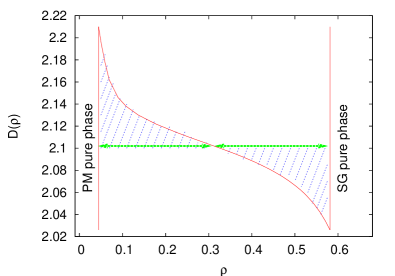
There are other two methods to determine a first order transition in
finite systems, based on the Maxwell construction. If we are in the
coexistence region the curve for the system of size will
display a sort of plateau around some : in a
very small interval of the density changes very rapidly. In
the case of a pure state, instead, the curve has a far
smoother behavior. In order to estimate the critical point we need to
extrapolate the behavior of for the pure phases inside the
region of coexistence. To this aim we perform two fits exclusively
based on the points outside the spinodal points: for
for the SG phase () and for the
PM phase ().
We will call
the inverse of the curves extrapolated from
the data points pertaining to the pure PM and SG phases,
respectively. The curve will denote the inverse of .
In this way we can make a
Maxwell-like construction in the , plane at a given
temperature and determine the value of as the one whose
corresponding value along the FS curve is equally
distant from both and ,
cf. Fig. 1:
| (23) |
IV.3 Maxwell “Equal area” estimate
Alternatively we can determine as the value at which, cf. Fig. 1
| (24) |
where and are arbitrary, provided that they pertain to the relative pure phases.
IV.4 Symmetric distribution estimate
Defining the skewness of the density probability distribution as
| (25) |
in Ref. [Katzgraber_skew, ] the critical point was estimated as the point at which the double peaked distribution is symmetric. Since the skewness of can be precisely computed this estimate does not suffer, e.g., of the arbitrariness of the choice of . In the thermodynamic limit, indeed, in the phase coexistence region both peaks of should be Dirac delta distributions and equal weight would be equivalent to a symmetric bimodal distribution. We will show the outcome of this analysis in our system for different cases and compare it with the previous ones.
V Exchange Monte Carlo algorithm in T and D
We have simulated our spin-1 model using the parallel tempering (PT) algorithm, replicating several copies of the system both at different temperatures and at different values of the external field . For the PT in temperature, the swap probability of two copies at temperature and is:
| (26) |
with ; whereas the swap probability in the chemical potential reads
| (27) |
We used the latter implementation in trying to identify the reentrance of the transition line in the plane. Since, however, the transition turns out to be first order in the whole region of inverse freezing, the PT algorithm must be handled with caution. Indeed, at the transition is discontinuous implying the vanishing of around the critical point for a given fix probe . In order to overcome this problem we have used a varying , smaller in the candidate coexistence region and larger and larger outside. An instance of this kind choice is represented in Fig. 2.
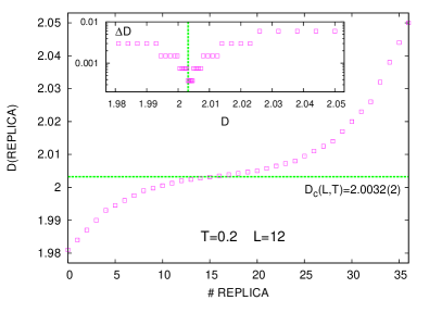
For very large sizes, though, this would require a too precise a-priori knowledge of the transition lines and the method could not be applied with a reasonable success. On the other hand, the FSS effects appear to be almost nonexistent at the first order phase transition, so that probes at larger sizes were actually not necessary. In Tabs. 1, 2 we report our simulation parameters for PT in temperature and in crystal field, respectively.
| 6 | 8 | 10 | 12 | 16 | 20 | 24 | ||
|---|---|---|---|---|---|---|---|---|
| 0.0 | ||||||||
| MCS | ||||||||
| 1.0 | ||||||||
| - | MCS | |||||||
| 1.75 | ||||||||
| - | MCS | |||||||
| 2.0 | ||||||||
| - | MCS |
| 6 | 8 | 10 | 12 | 15 | ||
|---|---|---|---|---|---|---|
| 0.2 | ||||||
| MCS | ||||||
| 0.3 | ||||||
| MCS | ||||||
| 0.4 | ||||||
| MCS | ||||||
| 0.5 | ||||||
| MCS |
Thermalization has been checked in three ways.
-
1.
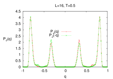
We have verified the symmetry with respect to zero of the site overlap distribution function for single random samples (cf, Fig. 3). In absence of an external magnetic field this must be symmetric for any choice of realization.
-
2.
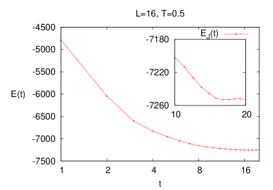
We have looked at the -log behavior of the energy and we have considered as thermalized those systems in which at least the last two points coincide within the error, cf. Fig. 3. This means that at least the last half of the data in MCS can be used for computing statistical ensemble averages.
-
3.
we have checked the lack of variation on logarithmic time-windows of all considered observables (e.g., and ) on at least two log points.
VI Numerical results.
VI.1 Second order phase transition and universality
In Fig. VI.1 we present the -behavior of for different values of and . In the first four cases the curves at different clearly cross, yielding evidence for a non zero . From a FSS we can, thus, extrapolate the critical temperature in the thermodynamic limit. The crossing points between curves are reported on column of Tab. 3. The FSS estimates are reported in columns and of Tab. 4, where couples are chosen both as (col. ) and as contiguous in the series (col. ). Analogous, though less precise estimates, can be obtained by studying the behavior of the Binder cumulant , cf. Eq. (17). Applying both the quotient and the conventional FSS methods we can, eventually, obtain two estimates for the critical exponents.
| * | * | |||||
| * | * | |||||
| * | * | |||||
| * | * | |||||
| * | * | |||||
Before applying these methods, though, we must check if we can exclude
cross-over effects as the chemical potential
is varied due to FS.
Since we are in presence of a tricritical point, signaled,
among others, by the weird behavior of at ,
cf. Fig. VI.1, we should control how it influences the
results as it is approached along the continuous transition line
increasing .
In the mean-field approximation, indeed, at the
tricritical point the coefficient of the fourth order term in the SG
free energy action goes to zero and the sixth order term becomes
relevant for the critical behavior, as shown in Ref.
[CLPRL02, ]. This is a typical behavior of Blume-Emery-Griffiths-Capel-like systems
Riedel72 ; ZZ that might hinder the determination of the critical
behavior in the neighborhood of the tricritical point for sizes that
are “not large enough”.
![[Uncaptioned image]](/html/1008.0024/assets/x5.png) Figure 4: Scaling functions vs. for different values
. For () evidence for a
continuous phase transition is found in the region of scale
invariance. At () no crossing is observed and,
at low , .
To estimate and control FS effects we use the scaling
methods introduced in Sec. III and compare different
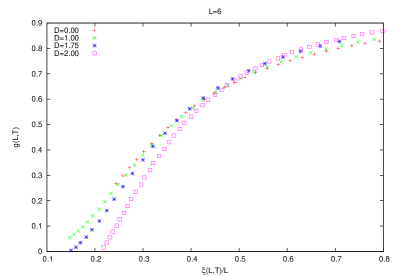
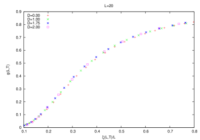
universal FSS functions. In Fig. 5 we plot the
Binder parameter vs. the rescaled correlation length at
all simulated values of the chemical potential both for a small
(, top) and a large (, bottom) system.
In the top plot one
can easily observe that as the tricritical value of is approached
() for the curves do not overlap with each
other signaling an apparent lack of universality. At large enough
sizes, instead, all curves are superimposed (bottom plot of
Fig. 5, ), demonstrating that universality
holds along the whole continuous transition line and that, because of
strong FS effects, a crossover occurs and the analysis limited to (or
including also) too small sizes can hinder the prediction of the
asymptotic behavior.
Figure 4: Scaling functions vs. for different values
. For () evidence for a
continuous phase transition is found in the region of scale
invariance. At () no crossing is observed and,
at low , .
To estimate and control FS effects we use the scaling
methods introduced in Sec. III and compare different
universal FSS functions. In Fig. 5 we plot the
Binder parameter vs. the rescaled correlation length at
all simulated values of the chemical potential both for a small
(, top) and a large (, bottom) system.
In the top plot one
can easily observe that as the tricritical value of is approached
() for the curves do not overlap with each
other signaling an apparent lack of universality. At large enough
sizes, instead, all curves are superimposed (bottom plot of
Fig. 5, ), demonstrating that universality
holds along the whole continuous transition line and that, because of
strong FS effects, a crossover occurs and the analysis limited to (or
including also) too small sizes can hinder the prediction of the
asymptotic behavior.
| * | * | |||||
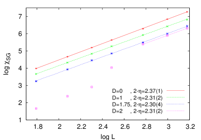
The same effect is clearly shown in Fig. 6 where the
size dependence of spin-glass susceptibility at criticality is shown.
As increases towards there appears to be a crossover
in the scaling moving from small to large sizes and induces wrong
asymptotic values of the critical indices.
We, thus, did not make use of the small values of for
, namely at and and at
, to interpolate the values of the critical exponents, as they
induce a wrong estimate as the limit is performed.
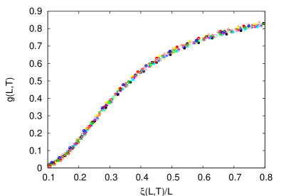
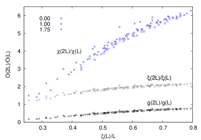
As a
test for the eye, in Fig. 7, we display
vs. for all and values employed for our FSS
analysis. Without the smallest sizes near the tricritical point,
universality appears quite tidy. In Fig. 8
we parametrically plot the universal FSS functions ,
and , cf. Sec. III, vs. ,
as well, for the same simulated systems.
The critical values of the temperature and the exponents and are shown in Tab. 4 both for the QM and the canonical FSS methods. Due to the FS cross-over no interpolation was possible with QM at . We, thus, provide only one estimate for the indeces.
| Model | ||
|---|---|---|
| SG 3D bd Jorg06 | 2.22(15) | -0.349(18) |
| SG 3D bd HPV08 | 2.53(8) | -0.384(9) |
| EA 3D BCPRB00 | 2.15(15) | -0.337(15) |
| EA 3D MPRPRB98 | 2.00(15) | -0.36(6) |
As one can see, comparing with estimates of critical exponents
summarized in Tab. 5, the system appears to be in the same
universality class of the Edwards-Anderson model (corresponding to the
limit of our model).BCPRB00 ; janus1 ; HTPV1 ; JK1
In Fig. VI.1 we also plot at
and for . In the first case we obtain a
, though no analysis of the critical exponents can be
performed because of FS effects. In the latter case no evidence is
found for a second order phase transition,
cf. Fig. VI.1. As is approached, moreover,
even appears to scale weaker than . We will see in the
following why this comes about.
VI.2 First order phase transition
Across a second order transition the system undergoes a transformation
from a PM pure phase to a SG pure phase. As far as the density
distribution is concerned, a pure phase corresponds to a
single-peaked distribution. As two peaks appear, the system exists
both in PM (low ) and SG (high ) coexisting phases and we
are in the neighborhood of a first order phase transition. In FS
systems the peaks are not delta-shaped but become sharper and sharper
as increases. At finite , thus, is a good order
parameter that drives the first order kind of transition: varying
, the system undergoes a transition with a discontinuous jump in
and the “thermodynamic” average values of
are obtained by looking at the peaks of its distribution.
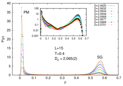
In Fig. 9 we show the behavior of the density
distribution through the first order transition at . The FS
first order transition points can be determined with the four methods
mentioned in Sec. IV, as we will show below. The spinodal
lines at given are estimated by looking at the values at which
a secondary peak arises.
Since the region of phase coexistence corresponds to an inverse freezing
transition, we performed PT
simulations at finite , changing .
Indeed, in our model, we will see that the first order transition line
displays a reentrance CLPRL05 ; LPM due to the existence of a
”fluid” (PM) phase with an entropy lower than the one of the glassy
phase.
For what concerns the estimate of the method of equal
weight introduced in Sec. IV, cf. Eq. (22) works
quite well for data collected at , because the two peaks
are very well separated as soon as they appear,
cf. Fig. 9, and the estimate is robust against
reasonable changes of (see inset of Fig. 9).
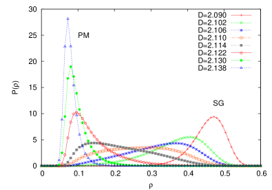
As increases towards the tricritical value, however, the PM and SG
values of the density approach each other. At ,
cf. Fig. 10, we thus have the problem that the
distributions of the densities of the two phases are overlapping also
for the largest simulated size. In that case, seen the arbitrariness
of choosing , we actually determine the transition point as
the value at which the peaks have the same height. This is a rough estimate
but yields no difference w.r.t., e.g., fitting the two peaks separately
and computing the areas under the interpolating curves. In
Tab. 6 we report for all simulated sizes and
temperatures the estimated values of the critical points obtained by
this method, together with the spinodal points.
These results can be cross-checked using the methods based on the Maxwell construction, cf. Sec. IV and Fig. 11. The pure phase behaviors are interpolated in the coexistence region by a polynomial fit on those points for which no double peak is present in the . At any given we look at the value such that (equal distance)
and at the value of at which the areas between and to the left and to the right of their crossing point are equal, i.e.,
| (28) |
is zero.
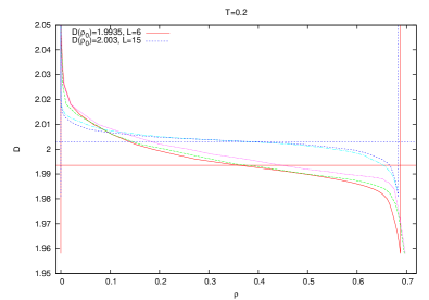
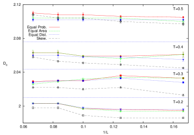
We, eventually, compute the skewness of double peaked as
changes, looking at the point for which .
Since the two peaks of at finite size appear to be of
different shape (SG broader, PM narrower),
cf. Figs. 9, 10, the point at which the
skewness is zero appears to be slightly different from the
values computed with the previous three methods. In
Fig. 12 we plot at different temperatures the FS values
of with the four methods. The equal weight methid and the
two Maxwell construction methods yield consistent results. For
the estimate of by the symmetric distribution
method displays a growing behavior in that does not allow for a
consistent , cf. Fig. 11 first and second
panel from top, whereas at lower temperature, where the interpolated
thermodynamic limit is stable the value is smaller than the other
estimates.
Summarizing, in Tab. 7 we report the estimates of the first order
critical point obtained by means of the four methods.
| T | ||||
|---|---|---|---|---|
| 0.2 | 2.0031(1) | 2.0033(2) | 2.0031(2) | 1.991(2) |
| 0.3 | 2.032(3) | 2.031(2) | 2.030(1) | 2.020(2) |
| 0.4 | 2.060(1) | 2.060(1) | 2.058(1) | x |
| 0.5 | 2.106(1) | 2.103(3) | 2.102(1) | x |
VI.3 Phase diagrams and inverse freezing
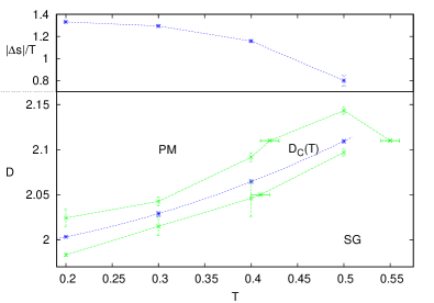
Phase diagrams are plotted in Fig. 13. In the plane we observe a pure SG phase at low and . Increasing the temperature the continuous transition to the pure PM phase is denoted by a full line connecting the five numerical estimates of obtained by simulations at and . We found no evidence for a continuous phase transition at . Beyond a tricritical point is placed. Beside changing to a first order transition, for lower also a reentrance in the line occurs. The warmest first order point for which we have an estimate is . In Fig. 14 a detail of the phase coexistence region is plotted (inside the grey-dotted lines). In the inset of Fig. 13 we plot the diagram. Below no pure phase exists with an average in between the dashed-grey curves.
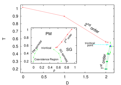
The inverse freezing takes place between a SG of high density to an almost empty PM
(e.g., at , in the coexistence region ,
and ). The few active
sites do not interact with each other but only with inactive neighbors
and this induces zero magnetization and overlap. The corresponding PM
phase at high has, instead, higher density (e.g.,
, )
and the paramagnetic behavior is brought about by the lack of both
magnetic order (zero magnetization) and blocked spin configurations
(zero overlap).
Using Eq. (21), from the
knowledge of and the numerical estimate of we
are able to evaluate the latent heat employed in the transition, that
we plot as a function of temperature in the top inset of
Fig. 14.
VII Nature of the SG phase.
The SG phase of the disordered BEG model, in mean-field regime, shows the same
features of the Sherrington-Kirkpatrick model:sk in order to
obtain a stable thermodynamics the Full RSB scheme is
needed.CLPRB04 ; CLPRL02 On the other hand, out of the limit of
validity of the mean-field regime, it is still unclear if the properties of SG
phase are in agreement with the RSB scenario.
The low phase is characterized by a pure spin-glass phase and
what this phase consists of in terms of statistical mechanic states is
the subject of the following analysis.
Three cases are contemplated in the
literature.
Droplet theory: it exists only one SG state (plus its symmetric
spin-reversed) and, therefore, the overlaps between states in
different replicas cannot fluctuate among different disordered samples
and the distributions are delta-shaped.droplet The four-spins
correlation function in position space
should tend to a plateau , for large enough , that
becomes longer as decreases towards .
Trivial-Non-Trivial (TNT) scenario: equilibrium states are many
and non-trivially organized (i.e., fluctuates from sample to
sample), but the excited states are droplet-like (i.e.,
the overlap, sensitive to interfaces, fluctuates less and less
as the size grows). This implies that is broad and
non-trivial, whereas is delta-shaped.tnt Since
excitations are trivial, the expected behavior of is the
same as for the droplet theory.
Replica Symmetry Breaking (RSB) theory: many states
characterize the SG phase, with space-filling excitations; both
distributions are, thus, broad, with a complex structure.
rsb ; MPV86 The correlation is expected to decay
continuously to zero (the minimum squared overlap for the present
system, in absence of an external magnetic field) at all
.Contucci07 ; Leuzzi08
First we will consider the overlap distribution functions,
cf. Eqs. (6)-(7), since, in the spin glass phase
(), the site and the link overlap distributions - and -
can be used as hallmarks to discriminate among different theories for
finite dimensional spin glasses. In the next section we will analyze
the four spin correlation functions.
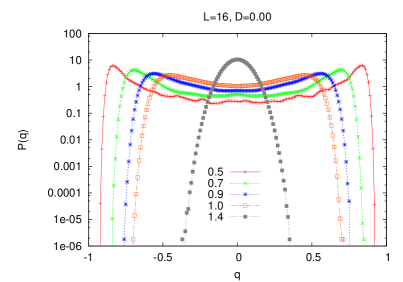
In order to see whether
is trivial or not we need to estimate if, for growing sizes its
support does shrink to a unique value, the Edwards-Anderson parameter
or it remains finite. In our case, in absence of an external magnetic
field, the support of a non-trivial should range from
to . In Fig. 15 we plot at
and size for all simulated temperatures: as decreases
moves from a Gaussian to a bimodal distribution. The
important issue is, then, whether the continuous part in between the
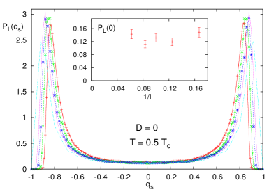
two peaks at low goes to zero or not as increases. In Fig. 16,
we plot at the lowest thermalized temperature for
and and, in the inset, we plot the values of
displaying no decreasing trend with increasing . The states, thus,
appear to be many and different among themselves, since they are found
with a finite probability within a non-zero continuous range of
overlap values, including .
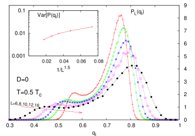
Also appears to develop a second peak at small as increases, and this signature becomes clearer and clearer at low temperature as increases, cf. Fig. 17. The analysis of FSS of the variance of might help to better evaluate the breadth of the distribution in the thermodynamic limit. Its behavior for various sizes is exemplified in the inset of Fig. 17 at the lowest we simulated for . The variance tends to a small finite value and we cannot make a definitive statement about tending towards a delta distribution, as conjectured by the TNT scenario. Moreover, the study of the variance does not yield any indication about the shape of the distribution. In particular, about the FSS behavior of the two peaks expected in RSB theory.
VII.1 Equivalence of site and link overlap distributions
We can, then, implement a more refined analysis of the pdf data and check whether and are actually equivalent and, thus, if the non-triviality of the former implies the non-triviality of the latter. This can be realized by recalling that in the SK model and by comparing to the distribution of an auxiliary variable
| (29) |
with a Gaussian random variable of variance and zero
mean, that mimics the presence of fluctuations due to the finite size
of the considered systems.
At a given point of the phase diagram and for a given
size , the parameters , and can be
obtained by minimizing the
Kullback-Leibler divergenceKL (KLD) between and :
| (30) |
We will refer to this one as the “left” KLD. The “right” KLD is the same formula exchanging and , where the symmetrized divergence (sKLD) between and is defined as: Leuzzi08
| (31) |
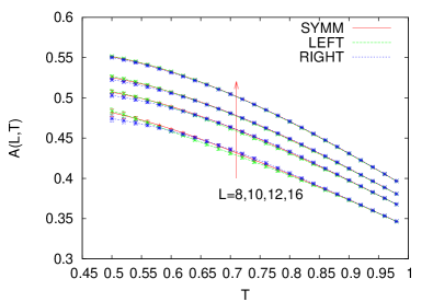
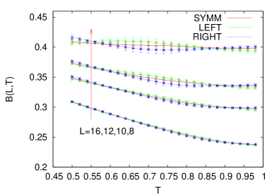
In Fig. 18 we plot, the finite size values of the parameters and . Besides the values of the parameters minimizing the symmetrized KLD, Eq. (31) we also plot the values of and minimizing the left and the right unsymmetrized KLD’s. We observe that, as increases the spread between different estimates tends to vanish. The infinite size limit of is always compatible with zero, signaling that FS effects actually tend to vanish as increases, though with large statistical errors at low temperature, implying that smaller sizes might hinder a correct FSS.
As instances we plot the matching of the two distributions and in Figs. 19 at and at size and .
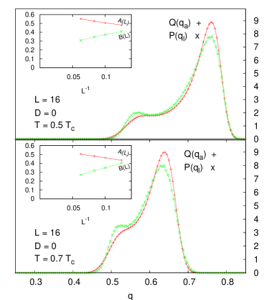
In the insets we plot the size behavior of and from the sKLD for the two specific cases. In the first case, performing a power-law FSS scaling to we obtain that interpolates a negative value! In the second case the limit yields a positive value. This observation is contrasting from the behavior, cf. bottom panel of Fig. 18, of growing with decreasing at all fixed sizes. Quite evidently, the low strong fluctuations strongly bias the interpolation at small . To show it in a clearer way, in Fig. 20 we plot the asymptotic values of both and for all simulated temperatures both from the sKLD and as the average of the extrapolation of the values minimizing the right and left unsymmetrized KLD’s. With the two estimates appear to be consistent at all temperature and reproduce the qualitative behavior detected in all finite cases, compare with Fig. 18. For , at low the two estimates are not consistent anymore. Moreover, decreases with below a certain , unlike its finite counterparts (at least as ), cf. Fig. 18.
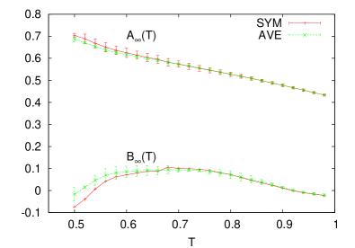
We face strong finite size effects and a crossover between small and large sizes is taking place. However, due to the fact that we cannot easily thermalize larger systems at low temperature, we cannot make any definite statement on the behavior of for very low . We simply do not have enough reliable points in at our disposal. The finite size behaviors, though, strongly suggest that and are, indeed, equivalent even below . In any case, the equivalence is proven for implying that not only the equilibrium states have a non-trivial distribution but also their excitations, yielding evidence in favor of the third scenario considered, the RSB theory, rigorously valid in mean-field systems.
VII.2 Position Space Four Spins Correlations
We now investigate the behavior of the four spins correlation
function, defined in Eq. (10), in position space. We
recall that the droplet and TNT theories predict that tends
to a plateau of height (cf. Sec. VII)
whereas RSB theory predicts for at a power-law decay
. We, thus, have to compare our data with the
prediction of one of these hypotheses.
Since we are dealing with small systems, we must first
consider possible FS effects. Indeed, because of the periodic
boundary conditions imposed on the simulated system, the correlation
function that we actually measure at a distance also contains the
contribution of correlations at distance , with
and the true (yet unknown) correlation function
is related to the measured one - - by
the relationship:
| (32) |
For large distances, when is smaller, these extra contribution
will strongly bias the estimate of the true behavior in
space. In particular, correlations at larger distances, of order ,
will experience relatively
stronger systematic errors than .
We will now present our results for the case . For
temperatures down to the critical region we simulated lattices with
sides of length up to . The largest thermalized size for
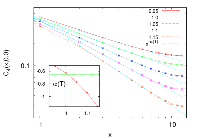
down to is, instead, . In Fig. 21 we
plot the behavior at in a log-log plot for the sizes
. One can observe that FS effects are limited to the
last point at . The rest of the curves completely superimpose.
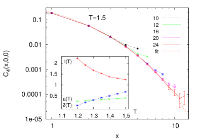
At high temperature, correlations are expected to decay exponentially at large enough distances. As temperature is lowered towards criticality the should become power-law eventually decaying as at . We, then, interpolate the four-spins correlation function along the -axis at criticality with the function:
| (33) |
and equivalently for and , due to the anisotropy of the system
in absence of an external field. This is a function containing a
crossover between a short distance power-law decay, , and
an exponential decay, with characteristic ’correlation’ length .
In Fig. 21 the function interpolating the
is plotted with ,
, with . As the
temperature decreases the correlation length increases until it
becomes too long to be observed in the analyzed systems. In the inset
of Fig. 21 we plot the behavior of ,
and until the fit becomes inconsistent .
In Fig. 22 we plot the curves at for sizes , as well as the interpolation of the
latter with (the correlation length is too long to
detect the exponential contribution in Eq. (33)). The
exponent equals the power at criticality
(at crystal field it was ,
cf. Tab. 3).
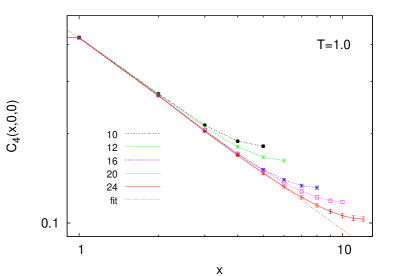
At the interpolated value of
for the curve is , for
and for . FS effects appear to be stronger now
w.r.t. Fig. 21 and evident also for (only points
for actually stay on the curve).
Approaching , as , cf. Fig. 23, it is
not possible to detect a crossover between power-law and exponential
decay and the simple power-law decay is tested. In the inset the power
behavior in is shown and compared with the power at criticality,
.
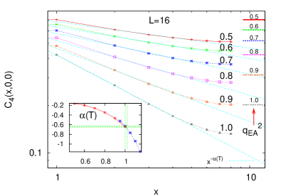
Decreasing further the temperature we show in Fig. 24 that the behavior is power-law until is reached. At that point the curves bend upwards as it did at criticality and even at high temperature, cf. Fig. 21. This bending is, however, an artifact due to the contributions induced by the periodic boundary conditions. In Fig. 24, on the right hand side, we show the values of at the same temperatures of the plotted . At all temperatures the soon decays below the corresponding value of . For the sizes simulated our data are, thus, not consistent with the observation of a plateau at as predicted by the droplet and TNT theories.
VIII Conclusions
In the present work we have performed Parallel Tempering Monte Carlo numerical simulations in the temperature/crystal field plane of the random 3D Blume-Capel model on a cubic lattice. This is a spin-1 spin glass, whose constituent features try to capture at least one supposed mechanism underlying inverse transitions: the raise of inactive components at low .
In particular, we have analyzed the second order phase transition
carrying out the computation of the critical temperatures and indeces
by means of parallel tempering simulations in temperature at different
values of the chemical potential . In this analysis we have
carefully checked FS effects, identified eventual crossovers from
small to large size scaling and neglected data for correspondingly too
small sizes. We verified that for different values of the system
is always in the same universality class (as far as a continuous
transition occurs) looking, e.g., at different universal scaling
functions of , such as the Binder parameter , or the
quotients of , and between systems at and .
The outcome is that at all the second order transition
belongs to the same universality class of the 3D Edwards-Anderson
model for spin-glasses.
We, then, estimated the position of a tricritical point, ,
, beyond which the transition is first order with jump in
density and in overlap parameters. This transition is first order in
the thermodynamic sense, i.e., latent heat is exchanged and, even
though the system is disordered, it is not related to the random
first order transition taking place in structural glasses.
LeuzziNieuw07 We employed and compared four different
methods to infer the critical line from FS data.
This observation confirms the claim
of Fernandez et al. Fernandez08 about the existence of
such transitions in quenched disordered short-range finite-dimensional
systems. In the present model the first order transition can be seen by
means of standard parallel tempering algorithm in the canonical ensemble,
simply tuning an external pressure-like parameter.
The first order transition line has the property of
displaying inverse freezing, as can be observed from the phase
diagram, cf. Figs. 13, 14: the low
temperature phase is paramagnetic and the system ’freezes’ into a
spin-glass phase as is increased. This is at difference with
the thermodynamic behavior of the original, ordered, BC model
(mean-field or finite dimensional). CapelPhys66 ; Saul74 In
presence of quenched disorder, a low temperature paramagnetic phase
exists that can acquire a very low density and this is the source of the
entropy decrease with respect to the high temperature paramagnetic
phase.
Both the inverse freezing transition and its first order nature
were not observed in the same model
on a hierarchical lattice. Ozcelik08
Eventually we present our analysis of the overlap distribution
functions and the four-spins correlation functions at criticality and
in the glassy phase, at for down to . From the
behavior of site overlap distribution at zero overlap, ,
and from the variance of the link-overlap distribution we
get evidence in favor of a complex organization of states in the SG
phase, displaying features typical of the Replica Symmetry Breaking
theory holding for mean-field systems (). We cross-checked
this observation comparing, with the Kullback-Leibler divergence, the
link-overlap distribution with the distribution of a function of the
squared site overlap, . We carefully analyzed the
finite size effects at low temperature finding that for small
size fluctuations strongly bias our estimates, yielding negative
coefficients of the term, decreasing with
temperature, unlike any finite size behavior. In order to have
a self-consistent estimate we would need to thermalize at systems of size sensitively larger than .
Looking at the position dependence of the four-spins correlation
functions we are able to detect, for , a crossover
between a short-distance power-law decay and a long-distance
exponential decay and we can identify a length-like parameter
playing the role of the correlation distance, growing as
decreases. As the critical temperature is approached and
becomes similar to the maximum feasible distance in the simulated
system (), can be interpolated with a simple
power-law. We checked that for sizes and the exponent
of at is equal to , where is the value
obtained from the analysis of the critical properties performed with
the quotient method. We also probed the power-law behavior for temperatures
down to at distances far away from border, where finite size correction
are too strong. Indeed, periodic boundary conditions systematically increase
correlations, above all where they are small (or vanishing), i.e., at large distance. We
compare the low temperature behavior with the prediction of TNT and
droplet theories that should tend to a plateau for large . Even though we are not able to reach
“large ”, we show that already at small
distance.
Acknowledgements.
We thank Nihat Berker, Helmut Katzgraber and Federico Ricci-Tersenghi for interesting discussions and exchanges.References
- (1) G. Tammann, “Kristallisieren und Schmelzen”, Metzger und Wittig, Leipzig (1903).
- (2) J. Wilks, D.S. Betts, An Introduction to Liquid Helium, Oxford University Press (USA, 1987).
- (3) S. Rastogi, G.W.H. Höhne and A. Keller, Macromolecules 32, 8897 (1999).
- (4) A.L. Greer, Nature 404, 134 (2000).
- (5) N.J.L. van Ruth and S. Rastogi, Macromolecules 37, 8191 (2004).
- (6) M. Plazanet et al. J. Chem. Phys. 121, 5031 (2004).
- (7) E. Tombari et al., J. Chem. Phys. 123, 051104 (2005).
- (8) M. Plazanet et al. J. Chem. Phys. 125, 154504 (2006).
- (9) M. Plazanet et al., Chem. Phys. 331, 35 (2006).
- (10) R. Angelini and G. Ruocco, Phil. Mag. 87, 553 (2007).
- (11) C. Ferrari et al., J. Chem. Phys. 126, 124506 (2007).
- (12) R. Angelini, G. Salvi and G. Ruocco, Phil. Mag. 88, 4109 (2008).
- (13) R. Angelini, G. Ruocco, S. De Panfilis, Phys. Rev. E 78, 020502 (2008).
- (14) M. Plazanet, M.R. Johnson and H.P. Trommsdorff, Phys. Rev. E 79, 053501 (2009).
- (15) R. Angelini, G. Ruocco and S. De Panfilis, Phys. Rev. E 79, 053502 (2009).
- (16) C. Chevillard and M.A.V. Axelos, Colloid. Polym. Sci. 275, 537 (1997).
- (17) M. Hirrien et al., Polymer 39, 6251 (1998).
- (18) A. Haque and E.R. Morris, Carb. Pol. 22, 161 (1993).
- (19) N. Avraham et al., Nature 411 451 (2001).
- (20) M. Greiner et al., Nature 415 39 (2002).
- (21) B. Donnio et al., Adv. Mater. 19, 3534 (2007).
- (22) B. Donnio et al., Soft Matter 6, 965 (2010).
- (23) E. Zaccarelli et al., Phys. Rev. E 63, 031501 (2002).
- (24) E. Zaccarelli et al. Phys. Rev. E 66, 04102 (2004).
- (25) P.E. Cladis, Phys. Rev. Lett. 35, 48 (1975);
- (26) P.E. Cladis, Phys. Rev. Lett. 39, 720 (1977);
- (27) H. Özbek et al., Ph. Trans. 75, 301 (2002);
- (28) O. Portmann, A. Vaterlaus, and D. Pescia, Nature 422, 701 (2003).
- (29) A. Srivastava, D. Sa and S. Singh, Eur. Phys. J. E 22, 111 (2007);
- (30) B. M. Jaffar Ali and A. Kumar, J. Chem. Phys. 107, 8020 (1997).
- (31) D. Bagchi, A.Kumar and R. Menon, J. Chem. Phys. 125, 034511 (2006).
- (32) H. Verbeek, G.J. Nieuwenhuys, H. Stocker, and J.A. Mydosh, Phys. Rev. Lett. 40, 586 (1978).
- (33) Y. Yeshurun, M.B. Salamon, K.V. Rao, and H.S. Chen, Phys. Rev. Lett. 45, 1366 (1980).
- (34) F.H. Stillinger, P.G. Debenedetti and T.M. Truskett, J. Phys. Chem. B 105, 11809 (2001).
- (35) F.H Stillinger and P.G. Debenedetti, Biophys. Chem. 105, 211 (2003).
- (36) M.R. Feeney., P.G. Debenedetti, and F.H. Stillinger, J. Chem. Phys. 119 4582 (2003).
- (37) N. Schupper and N.M. Shnerb, Phys. Rev. Lett. 93 (2004) 037202.
- (38) N. Schupper and N.M. Shnerb, Phys. Rev. E, 72: 046107, 2005.
- (39) S. Prestipino, Phys. Rev. E 75, 011107 (2007).
- (40) A. Crisanti and L. Leuzzi, Phys. Rev. Lett. 95, 08720170 (2005).
- (41) M. Sellitto, Phys. Rev. B 73 180202 (2006).
- (42) M. Sellitto and J. Kurchan, Phys. Rev. Lett. 95, 236001 (2005).
- (43) A. Allahverdyan and Petrosyan, Phys. Rev. Lett. 96, 065701 (2006).
- (44) H. W. Capel, Physica 32(1966) 966; M. Blume, Phys. Rev. 141 (1966) 517.
- (45) S. K. Ghatak, D. Sherrington, J. Phys. C: Solid State Phys. 10, 3149 (1977).
- (46) J. Dumas et al., Phys. Rev. B 20, 3913 (1979).
- (47) A. Crisanti and L. Leuzzi, Phys. Rev. Lett. 89 (2002) 237204.
- (48) A. Crisanti and L. Leuzzi, Phys. Rev. B 70 (2004) 014409.
- (49) L. Leuzzi, Phil. Mag. 87, 543-551 (2006).
- (50) M. Blume, V.J. Emery and R.B. Griffiths, Phys. Rev. A 4 (1971) 1071.
- (51) D.M. Saul, M. Wortis and D. Stauffer, Phys. Rev. B 9, 4964 (1974).
- (52) A. Nihat Berker and M. Wortis, Phys. Rev. B 14, 4946 (1976).
- (53) A. K. Jain and D. P. Landau, Phys. Rev. B 22, 445 (1980).
- (54) M. Hasenbusch, arXiv:1004.4983v1.
- (55) V.O. Özçelik and A. N. Berker, Phys. Rev. E 78, 031104 (2008).
- (56) L.A. Fernàndez et al., Phys. Rev. Lett. 100, 057201 (2008).
- (57) F.P. Toldin, A. Pelissetto and E. Vicari, J. Stat. Phys. 135, 1039 (2009).
- (58) M. Paoluzzi, L. Leuzzi and A. Crisanti, Phys. Rev. Lett. , (2010).
- (59) K. Hukushima and K. Nemoto, J. Phys. Soc. Jpn. 65, 1604 (1996).
- (60) E. Marinari, Adv. Computer Simul. 501, 50 (1998).
- (61) M. Mèzard, G. Parisi and M. A. Virasoro, Spin glass theory and beyond (Word Scientific, Singapore 1987)
- (62) S. Caracciolo et al., Nucl. Phys. B403, 475 (1993).
- (63) M. Palassini, S. Caracciolo, Phys. Rev. Lett. 82, 5128 (1999).
- (64) W. Kauzmann, Chem. Rev. 43, 219 (1948).
- (65) T.L. Hill, Thermodynamics of Small Systems, Dover (2002).
- (66) R.S. Andrist, H.G. Katzgraber, H. Bombin, M.A. Martin-Delgado, arXiv:1005.0777v1.
- (67) E.K. Riedel and F.J. Wegner, Phys. Rev. Lett. 29, 349 (1972).
- (68) J. Zinn-Justin, Quantum Field Theory and Critical Phenomena, Oxford University Press (Oxford, 1989).
- (69) T. Jörg, Phys. Rev. B 73, 224431 (2006).
- (70) M. Hasenbusch, A. Pelissetto, E. Vicari, J. Stat. Mech. L02001, (2008).
- (71) H. G. Ballesteros et al., Phys. Rev. B 62 (2000) 14237.
- (72) E. Marinari, G. Parisi and J. J. Ruiz-Lorenzo Phys. Rev. B 58 (1998) 14852.
- (73) F. Belletti et al., Phys. Rev. Lett. 101 157201 (2008).
- (74) M. Hasenbusch, F. P. Toldin, A. Pellissetto, and E. Vicari, Phys. Rev. B 76, 094402 (2007); ibid. 184202 (2007).
- (75) T. Jorg, H. G. Katzgraber, Phys. Rev. Lett. 101, 197205 (2008); Phys. Rev. B 77, 214426 (2008).
- (76) D. Sherrington, S. Kirkpatrick, Phys. Rev. Lett. 35, 1792 (1975).
- (77) D. S. Fisher, D.A. Huse, Phys. Rev. Lett. 56, 1601 (1986).
- (78) F. Krzakala, O.C. Martin, Phys. Rev. Lett. 85, 3013 (2000).
- (79) G. Parisi, Phys. Lett. A 73 203-205 (1979), J. Phys. A 13, L115 (1980), Phys. Rev. Lett. 50 1946-1948 (1983).
- (80) S. Kullback and R.A. Leibler, Ann. Math. Stat. 22, 79 (1951).
- (81) P. Contucci et al., Phys. Rev. Lett. 99, 057206 (2007).
- (82) L. Leuzzi, G. Parisi, F. Ricci-Tersenghi, J.J. Ruiz-Lorenzo, Phys. Rev. Lett. 101, 107203 (2008).
- (83) L. Leuzzi and T.M. Nieuwenhuizen, Thermodynamic of the glassy state, Taylor & Francis (2007).