Intrinsic selection biases of ground-based gravitational wave searches for high-mass BH-BH mergers

Abstract

The next generation of ground-based gravitational wave detectors may detect a few mergers of comparable-mass $M\simeq 100-1000M_{\odot}$ (“intermediate-mass”, or IMBH) spinning black holes. Black hole spin is known to have a significant impact on the orbit, merger signal, and post-merger ringdown of any binary with non-negligible spin. In particular, the detection volume for spinning binaries depends significantly on the component black hole spins. We provide a fit to the single-detector and isotropic-network detection volume versus (total) mass and arbitrary spin for equal-mass binaries. Our analysis assumes matched filtering to all significant available waveform power (up to $l=6$ available for fitting, but only $l\leq 4$ significant) estimated by an array of 64 numerical simulations with component spins as large as $S_{1,2}/M^{2}\leq 0.8$. We provide a spin-dependent estimate of our uncertainty, up to $S_{1,2}/M^{2}\leq 1$. For the initial (advanced) LIGO detector, our fits are reliable for $M\in[100,500]M_{\odot}$ ($M\in[100,1600]M_{\odot}$). In the online version of this article, we also provide fits assuming incomplete information, such as the neglect of higher-order harmonics. We briefly discuss how a strong selection bias towards aligned spins influences the interpretation of future gravitational wave detections of IMBH-IMBH mergers.

I Introduction

Ground-based gravitational wave detectors like LIGO and Virgo are presently taking data at and beyond design sensitivity Acernese et al. (2006); Abbott et al. (2003) (The LIGO Scientific Collaboration). Over the next several years as upgrades are performed, these detectors’ sensitivity will increase substantially Shoemaker and the LIGO Scientific Collaboration (2009). Advanced detectors are very likely to see many few-stellar-mass black hole binaries formed through isolated O’Shaughnessy et al. (2009); Belczynski et al. (2010) and dynamical O’Shaughnessy et al. (2007); Sadowski et al. (2008); Banerjee et al. (2010) processes. Additionally, advanced detectors could see the merger signature of two intermediate-mass black holes (each $M\in[100,10^{3}]$), binaries which might be formed in dense globular clusters Fregeau et al. (2006). Unless astrophysical processes strongly suppress black hole spin, that spin will have a substantial effect on all the components of the signal to which these ground-based detectors are sensitive: the late-time inspiral, merger signal, and (through the final BH spin) ringdown. Though analytic approximations exist to describe the early-time (inspiral) and late-time (ringdown) behavior of a spinning BH-BH binary, the merger signal must be obtained numerically, in principle for all possible mass ($m_{1},m_{2}$) and spin (${\mathbf{S}}_{1},{\mathbf{S}}_{2}$) combinations. Of the types of black holes likely to be detected in the near future, intermediate-mass black holes have masses and spins such that their entire (short) detectable waveform is dominated by the merger signal. As a result, very few candidate intermediate-mass merger waveforms are presently available, particularly for generic spins Lousto et al. (2010); Campanelli et al. (2009); Szilágyi et al. (2009); Campanelli et al. (2010). Conversely, the performance of real gravitational wave search pipelines is difficult to assess without extensive Monte Carlo simulations. All searches suffer from highly nongaussian noise and time-variable detector performance; matched filter searches adopt a range of approximate waveforms, coincidence, and nongaussian-noise rejection strategies. However, given the computational burden of each NR simulation and the limited selection currently available, extensive Monte Carlo studies are not presently practical. Nonetheless, all numerical simulations to date suggest that gravitational merger waveforms are surprisingly simple. For example, for aligned spin both the final spin Rezzolla (2009); Marronetti et al. (2008); Barausse and Rezzolla (2009); Kesden et al. (2010) and even merger waveforms Ajith et al. (2009); Reisswig et al. (2009a); Pan et al. (2010) have been accurately fit, for all possible component masses $(m_{1},m_{2})$ and spin magnitudes $|{\mathbf{S}}_{1}|,|{\mathbf{S}}_{2}|$ for moderate spin magnitude ($<0.9$) and mass ratio ($<1/10$), for the dominant mode of radiation.

Given the simplicity of numerical merger waveforms and the few available simulations, in this paper we outline a simple method to analytically estimate the performance of present and future gravitational wave searches, extrapolating from a small array of existing numerical simulations. Our method relies only on the raw numerical simulation output and detector response functions; we neither model the waveform itself nor limit to a few “dominant harmonics” associated with the early- or late-time binary orientation. In Sec. II we describe (i) how we estimate the detection volume of present and future gravitational wave searches for comparable mass binaries with known waveforms and (ii) how we extrapolate between them using fits. In Sec. III and Table 2 we describe the set of NR simulations used. In Sec. IV, we compare our results on aligned spin to previously published estimates. Additionally, we use our aligned spin results to emphasize how sensitive our predictions are to small systematic issues such as wave extraction radius and (to a lesser extent) numerical resolution. Then, in Sec. V we provide the coefficient functions needed for arbitrary spins with total and incomplete ($l_{max}=2,3,4,\ldots$) waveform catalogs, along with our best estimates for parameter-dependent uncertainty in the detection volume. Finally, in Sec. VI we discuss how much (or little) spin influences searches for high-mass IMBH-IMBH mergers.

II GW Searches for high-mass mergers: Selection biases

The sensitivity of a network of gravitational wave detectors to a single class of randomly oriented source is often characterized in three ways: (A) via the maximum amplitude an optimally oriented but otherwise identical binary produces; (B) using the angle-averaged signal power $\bar{\rho}_{*}$ incident on a single detector Flanagan and Hughes (1998) from sources at a fixed distance; (C) via the expected detection rate for that class of source O’Shaughnessy et al. (2009), adopting a distribution $p(\lambda)$ of sources described by parameters $\lambda$ ($=$ component masses $m_{1},m_{2}$; spins ${\mathbf{S}}_{1},{\mathbf{S}}_{2}$; emission direction ${\mathbf{\hat{n}}}$ in the frame of the binary; sky location and polarization angle $\hat{N},\psi$; and distance $r$). For example, for a single interferometer with Gaussian noise, the signal-to-noise ratio $\rho_{*}(\lambda)$ can be expressed as

$$h_{det}(t) = F_{+}(\hat{N},-\psi)h_{+}({\mathbf{\hat{n}}},t)+F_{\times}(\hat{N},-\psi)h_{\times}({\mathbf{\hat{n}}},t)$$

$$\left<a|b\right> \equiv 2\int_{-\infty}^{\infty}df\frac{\tilde{a}(f)^{*}\tilde{b}(f)}{S_{h}(f)}$$ (1)

$$\rho_{*}^{2} = \left<h_{det}|h_{det}\right>$$ (2)

where $F_{+,\times}$ are standard single-detector beampattern functions and where we use a subscript $*$ when referring to a single detector; compare to Appendix C. For the first method, a peak signal to noise $\rho_{*,max}$, is particularly useful for aligned or nonspinning binaries dominated by $l=|m|=2$ emission, where the relative change in $\rho$ versus $\hat{N},\psi,{\mathbf{\hat{n}}}$ is known analytically; see, e.g., Eq. (2) in O’Shaughnessy et al. (2009). In the second method, the source- and sky-location-averaged signal power incident on a single detector leads naturally to orientation-averaged power over a complex wave amplitude

$$\bar{\rho}_{*}^{2} = \left<\left<h_{det}|h_{det}\right>\right>_{\psi,\hat{n},\hat{N}}\equiv\int\frac{d\Omega_{N}d\Omega_{n}}{(4\pi)^{2}}\frac{d\psi}{\pi}\left<h_{det}|h_{det}\right>$$

$$= \int\frac{d\Omega_{n}}{4\pi}\int\frac{d\Omega_{N}d\psi}{4\pi^{2}}\left[F_{+}^{2}\left<h_{+}|h_{+}\right>+0+F_{\times}^{2}\left<h_{\times}|h_{\times}\right>\right]$$

$$= \frac{1}{5}\int\frac{d\Omega_{n}}{4\pi}[\left<h_{+}|h_{+}\right>+\left<h_{\times}|h_{\times}\right>]$$

$$= \frac{1}{5}\bar{\rho}^{2}$$ (4)

where $\bar{\rho}^{2}$ is a technically convenient lower-dimensional average with clear physical meaning – the average over all source orientations of the network signal-to-noise recovered by either (i) a pair of identical detectors, oriented at $45^{o}$ to each other and with the source directly overhead, or equivalently (ii) a network of detectors with equal sensitivity to both polarizations in all directions [cf. Appendix C]:

$$\bar{\rho}^{2} \equiv \int\frac{d\Omega_{n}}{4\pi}\left<h_{+}+ih_{\times}|h_{+}+ih_{\times}\right>_{\text{fixed }\hat{n}}\;,$$ (5)

Thus, the orientation-averaged power is technically convenient since, if the emitted waveform is expressed as an expansion of the asymptotic complex waveform $h_{+}+ih_{\times}$ or curvature scalar $\Psi_{4}$ into spin-weighted spheroidal harmonics

$$h_{+}+ih_{\times} = \sum_{lm}h_{lm}(t)\,{}_{-2}Y_{lm}\,,$$ (6)

then the angle-averaged signal power becomes a sum over inner products of the harmonic amplitude functions $h_{lm}$ or (with a different inner product) $\Psi_{4,lm}$ given by

$$\bar{\rho}^{2} = \sum_{lm}\frac{\left<h_{lm}|h_{lm}\right>}{4\pi}$$

$$= \sum_{lm}\frac{1}{2\pi r^{2}}\int_{0}^{\infty}\frac{df}{(2\pi f)^{4}S_{h}}\left[|\tilde{\Psi}_{4,lm}(f)|^{2}+|\tilde{\Psi}_{4,lm}(-f)|^{2}\right]$$

$$\equiv \sum_{lm}(\Psi_{4,lm}|\Psi_{4,lm})\,;$$ (8)

see, for example, Eqs. (7,8) in Reisswig et al. (2009a). For clarity we have described both methods (A) and (B) as a characteristic SNR $\rho$ for sources at a fixed distance, adopting a detection-strategy-neutral characterization. If one adopts a fiducial signal to noise ratio $\rho_{c}$, such as a cutoff for single-detector SNR, then these amplitudes convert to physical distances; for instance, (B) implies an angle-averaged reach $\bar{D}_{*}$ defined by the solution to $\bar{\rho}_{*}(\bar{\lambda},D)=\rho_{c}$, or equivalently by

$$\bar{\rho}_{*}(\bar{\lambda}) = \rho_{c}\frac{\bar{D}_{*}(\bar{\lambda})}{r}$$ (9)

where $\bar{\lambda}=(m_{1},m_{2},{\mathbf{S}}_{1},{\mathbf{S}}_{2}$ and suitable orbital phases) are the physical (“intrinsic”) parameters of the binary (i.e., all parameters except $\psi,N,n$ and distance).

Though well-defined, both methods only approximate the astrophysically-relevant sensitivity of gravitational wave detectors to spinning systems. For example, both the distribution and even optimal emission direction ($\psi,{\mathbf{\hat{n}}}$) depend strongly on the direction of the total angular momentum $J$ in band; and, therefore, on the masses and spins involved. While the peak amplitude could easily be tabulated and fit following the procedure described below, for astrophysical purposes (A) and (B) alone lose information about the beampattern shape function needed to construct (C), the astrophysically-relevant measure of sensitivity. To encapsulate all needed information about the beampattern shape, we introduce a beampattern function $w_{*}$ for the ratio of single-detector SNR $\rho$ to orientation-averaged single-detector SNR $\bar{\rho}_{*}$:

$$w_{*} \equiv \rho_{*}(\lambda)/\bar{\rho}_{*}(\bar{\lambda})$$ (10)

$$\rho_{*} = \frac{\rho_{c}\bar{D}_{*}(\bar{\lambda})w_{*}(\hat{N},{\mathbf{\hat{n}}},\psi|\bar{\lambda})}{r}\,.$$ (11)

By construction, the orientation average of $w^{2}_{*}$ is always exactly unity ($\left<w^{2}_{*}\right>=1$). In terms of this beampattern function and the previously defined angle-averaged range $\bar{D}$, the detection rate for sources in the nearby universe can be expressed as a sum over the rate per unit physical volume $dV=r^{2}drd\Omega_{N}$ and per volume in binary parameters $d\lambda=d\Omega_{source}d\bar{\lambda}$:

$$R_{D} = \int_{\rho>\rho_{c}}\frac{dN}{dtdVd\lambda}dVd\lambda$$

$$= \int\frac{dN}{dtdV}p(\bar{\lambda})d\bar{\lambda}\int\frac{d\Omega_{source}}{\Omega_{source}}\int_{\rho_{*}>\rho_{c}}dV\,.$$

The last factors represent the detection volume averaged over source orientations. In the nearby universe, this orientation-averaged detection volume can be evaluated, reducing the detection rate to

$$= \frac{dN}{dtdV}\int p(\lambda)d\lambda\;\frac{4\pi}{3}(\bar{D}_{*}\bar{w}_{*})^{3}\,,$$ (12)

which shows that the final detection rate can be explained as a product of: (i) total event rate per unit volume $\frac{dN}{dtdV}$; (ii) distribution of events in parameters; and a (iii) source-frame-averaged volume that characterizes the typical reach to sources with parameters $\lambda$, consisting of (iv) an orientation-averaged range $\bar{D}_{*}$, proportional to the band-limited SNR $\bar{\rho}_{*}$ for a source at a fixed distance, and (v) a beaming correction factor $\bar{w}_{*}$, that depends on how the binary’s polarized, beamed emission interacts with our network’s polarization-dependent beampattern. In other words, the angle-averaged reach $\bar{D}_{*}$ almost describes the astrophysically relevant reach, modulo a weak correction factor

$$\bar{w}_{*}(\bar{\lambda}) \equiv \frac{\int\frac{d\Omega_{n}d\Omega_{N}d\psi}{4\pi(4\pi)(\pi)}\left[w_{*}({\mathbf{\hat{n}}},\psi,\hat{N}|\bar{\lambda})^{3}\right]^{1/3}}{\left<w^{2}_{*}\right>^{2/3}}$$ (13)

which, like $\bar{\rho}$, can be tabulated and fit versus all intrinsic parameters $\bar{\lambda}$. As we will see below, the beampattern correction function average $\bar{w}_{*}$ is necessarily almost always unity, with $\bar{w}_{*}-1$ largest for aligned binaries and exactly zero for isotropic emission. In fact, given the uncertainties expected in our fit to $\bar{\rho}(\lambda)$, an excellent first approximation to $\bar{w}_{*}$ is unity.

Fit versus spin

Owing to the relative simplicity of numerical merger waveforms, scalar functionals of the waveforms like the final mass $M_{f}$ and spin $J_{f}^{2}$ can be fit across the entire space of intrinsic parameters $\bar{\lambda}$ Boyle and Kesden (2008). Fits for the remnant BH’s recoil kick and spin have been extensively explored in the literature Boyle and Kesden (2008); Boyle et al. (2007); Rezzolla et al. (2008a, b); Baker et al. (2008a); Rezzolla (2009); Barausse and Rezzolla (2009). Experience from fitting the final spins and signal-to-noise-ratio of aligned spinning binaries [Sec. IV] suggests an accurate fit to $\bar{\rho}({\mathbf{S}}_{1},{\mathbf{S}}_{2})$ requires at least cubic order in the components of $S_{1,2}$ along the early-time orbital angular momentum direction $\hat{L}$ (henceforth denoted ${\mathbf{\hat{z}}}$). Though a generic symmetry-preserving expansion contains many components (roughly $6^{3}/4$ in a cubic-order expansion of a six-dimensional space with two $Z_{2}$ symmetries, parity and black hole exchange), the physics of a precessing merging binary strongly suppresses most terms. A truly generic symmetry preserving expansion of a scalar function allows scalar functions of ${\mathbf{S}}_{1},{\mathbf{S}}_{2}$ to have a preferred spin direction perpendicular to the total angular momentum, along the axis connecting the two holes at our simulations’ starting time. Precession rapidly evolves in-plane spin components away from this preferred axis. We anticipate and test simulations confirm minimal dependence of the amplitude $\bar{\rho}$ on the relative orientation of spins to this preferred axis.

For this reason, rather than use all spin components, as in Boyle and Kesden (2008), we describe our expansion in terms of three quantities: the preferred out of plane direction ${\mathbf{\hat{z}}}\propto J$; the in-plane projection operator $P$ perpendicular to ${\mathbf{\hat{z}}}$; and a pair even- and odd- exchange-symmetric reduced spins:

$$\boldsymbol{\chi}_{\pm} = (m_{1}a_{1}\pm m_{2}a_{2})/M\qquad[\boldsymbol{\Sigma}\propto-{\boldsymbol{\chi}_{-}}]$$ (14)

where $a_{k}=S_{k}/m_{k}^{2}$. An exchange-symmetric expansion of equal-mass binaries must have even powers of ${\boldsymbol{\chi}_{-}}$. [For unequal masses, terms proportional to ${\boldsymbol{\chi}_{-}}$ are possible when prefixed by asymmetric mass terms. A generic expansion will introduce at linear spin order $(\delta m/M)({\boldsymbol{\chi}_{-}}\cdot{\mathbf{\hat{z}}})$, at quadratic spin order $(\delta m/M)P{\boldsymbol{\chi}_{-}}\cdot P{\boldsymbol{\chi}_{+}}$, et cetera. The exchange-symmetric coefficients provided below can depend on only even powers of $(\delta m/M)$.] Working to cubic order, we anticipate $\bar{\rho}$ has the form

$$\bar{\rho}(m_{1},m_{2},{\mathbf{S}}_{1},{\mathbf{S}}_{2}) = \bar{\rho}_{o}(m_{1},m_{2})[1$$

$$+ {\cal X}_{1}({\boldsymbol{\chi}_{+}}\cdot z)+{\cal X}_{2}({\boldsymbol{\chi}_{+}}\cdot{\mathbf{\hat{z}}})^{2}+{\cal X}_{3}({\boldsymbol{\chi}_{+}}\cdot{\mathbf{\hat{z}}})^{2}$$

$$+ {\cal X}_{02}(P{\boldsymbol{\chi}_{+}})^{2}+{\cal A}_{20}({\boldsymbol{\chi}_{-}}\cdot z)^{2}+{\cal A}_{02}(P{\boldsymbol{\chi}_{-}})^{2}$$

$$+ {\cal B}_{1200}({\boldsymbol{\chi}_{+}}\cdot z)(P{\boldsymbol{\chi}_{+}})^{2}$$

$$+ {\cal B}_{1020}({\boldsymbol{\chi}_{+}}\cdot z)({\boldsymbol{\chi}_{-}}\cdot z)^{2}$$

$$+ {\cal B}_{1002}({\boldsymbol{\chi}_{+}}\cdot z)(P{\boldsymbol{\chi}_{-}})^{2}+O(\chi^{4})\ldots]$$

$$\bar{w}_{*}(m_{1},m_{2},{\mathbf{S}}_{1},{\mathbf{S}}_{2}) = \bar{w}_{o,*}(m_{1},m_{2})[1$$

$$+ {\cal Z}_{1}{\boldsymbol{\chi}_{+}}\cdot{\mathbf{\hat{z}}}+{\cal Z}_{2}({\boldsymbol{\chi}_{+}}\cdot{\mathbf{\hat{z}}})^{2}\ldots$$

$$+ {\cal C}_{20}({\boldsymbol{\chi}_{-}}\cdot{\mathbf{\hat{z}}})^{2}+{\cal C}_{02}(P{\boldsymbol{\chi}_{-}})^{2}+\ldots$$

$$+ {\cal D}_{1200}({\boldsymbol{\chi}_{+}}\cdot z)(P{\boldsymbol{\chi}_{-}})^{2}+\ldots$$

$$= 1.095[1+{\cal Z}_{1}{\boldsymbol{\chi}_{+}}\cdot{\mathbf{\hat{z}}}+\ldots]$$

where $\bar{\rho}_{o}(m_{1},m_{2})$ is provided by a comparable calculation for nonspinning binaries and where the value for $\bar{w}_{o*}$ for ${\mathbf{S}}_{1}={\mathbf{S}}_{2}=0$ shown can be estimated using only the dominant $l=|m|=2$ aligned emission beampattern. In most of the text we will refer explicitly to the coefficient functions described above. However, when referring to this expansion in its entirety, we adopt the shorthand abstract notation $y_{\alpha}$ for its coefficient functions (of $M$) and $\psi_{\alpha}$ for basis functions (of $\chi_{\pm}$):

$$\bar{\rho}/\bar{\rho}_{o}=\sum_{\alpha}\psi_{\alpha}y_{\alpha}\,.$$ (17)

For equal-mass binaries $m_{1}=m_{2}=M/2$, we determine the coefficient functions ${\cal X}_{1,2,3}(M),\ldots$ suitable to a specific gravitational wave detector noise power spectrum $S_{h}$ as follows. We pick a total mass $M$. For all numerical simulation $k$ in Table 2, corresponding to spin combinations $S_{1,k},S_{2,k}$, we extract time domain spin-weighted harmonics of the Weyl scalar $\Psi_{4,lm,k}(t)$ for $l\lesssim 6$. We construct each $\bar{\rho}_{k}$ using Eq. (8). Likewise, we construct $\bar{w}$ by (i) reconstructing $\tilde{h}$ along a large number of randomly chosen orientations ($\hat{N},\psi,{\mathbf{\hat{n}}}$), using the multipole coefficients $\tilde{\Psi}_{4,lm}$; (ii) calculating $w_{*}^{3}$; then (iii) averaging over all the random samples. Finally, excepting only a few simulations chosen as blind tests of our fit [Sec. 8], we perform a simple least-squares fit for the coefficients $y_{\alpha}$ in Eq. (II), adopting uniform uncertainties in $\rho_{k}$ for all $k$. Since $\bar{w}$ varies little from unity and since our estimate is subject to significant Poisson sampling error, we retain only leading-order dependence with spin (${\cal Z}_{1}$).

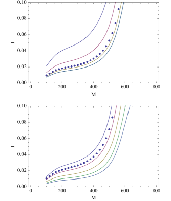
Fit errors: Numerical, systematic, and truncation errors limit our ability to determine these coefficients precisely. High-order or symmetry-suppressed coefficients like ${\cal X}_{3}$ and ${\cal A}_{20}$ are particularly sensitive to small numerical errors. Furthermore, the recovered coefficients $y_{\alpha}(M)$ have highly correlated uncertainties $\Sigma_{\alpha\beta}(M)$, where $\Sigma_{\alpha\beta}$ is the least-squares estimate of the parameter covariance matrix. Finally, phenomenologically speaking the interesting uncertainty is how much our fit $\hat{F}$ to our data, say for $\bar{\rho}$,

$$F_{k}=\bar{\rho}_{k}/\bar{\rho}_{o}\,,$$

differs from truth. Though highly dependent on the parameter distribution of simulations used in the fit, one simple estimate for overall error is the residual rms error between the data and our least-squares fit:

$$\delta F^{2}=\sum_{k}(\hat{F}(\lambda_{k})-F_{k})^{2}/N\,.$$

A far more stable and spin-magnitude-dependent representation of fit uncertainty is the expected $L^{2}$ error ${\cal F}(a)$ in the fit for spins with magnitude ${\mathbf{S}}_{1}/m_{1}^{2},{\mathbf{S}}_{2}/m_{2}^{2}\leq a$:

$${\cal F}^{2}(a) = \left<(\bar{\rho}-\left<\bar{\rho}\right>)^{2}\right>_{fit}/\bar{\rho}_{o}^{2}$$ (18)

$$\equiv \sum_{ab}\Sigma_{ab}\left<\psi_{a}\psi_{b}\right>_{spins}a^{s_{a}+s_{b}}$$

where we use integer exponents $s_{a}$ to describe the order of the basis functions ($\psi_{a}(x{\mathbf{S}}_{1},x{\mathbf{S}}_{2})=x^{s_{a}}\psi_{a}({\mathbf{S}}_{1},{\mathbf{S}}_{2})$); where $\Sigma_{\alpha,\beta}$ is the least-squares covariance matrix of fit parameters; and where the coefficients are easily-tabulated moments of the coefficient matrix over all spins, provided in Table 1:

$$\left<\psi_{a}\psi_{b}\right>_{all} = \int_{|a_{1,2}|<1}\frac{d^{3}a_{1}d^{3}a_{2}}{(4\pi/3)^{3}}\psi_{a}(a_{1},a_{2})\psi_{b}(a_{1},a_{2})\,.$$ (19)

Roughly speaking, ${\cal F}(a)$ estimates the relative error in $\bar{\rho}$ when applying our fit to a generic pair of spins with typical magnitude $a$.

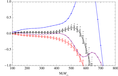
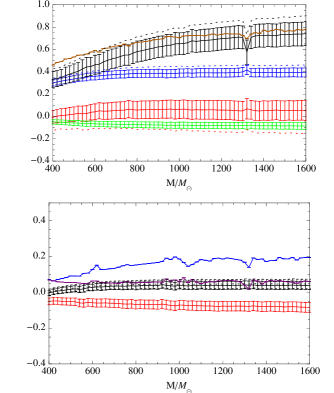
Astrophysical tolerance: Astrophysically speaking, the orientation-averaged range relates the number of sources observed (or their absence) to the implied source event rate (or upper bound). Even adopting the most optimistic assumptions, no more than $O(10)$ intermediate-mass mergers are expected to be seen by advanced ground-based detectors Fregeau et al. (2006), at best allowing the source event rate be determined to $O(30\%)$ at $1\sigma$ confidence. To achieve this level of accuracy, we require only $O(10\%)$ accuracy in $\bar{D}\bar{w}$. Even for maximally rotating black holes, our fits should be at least that accurate; see Fig 1.

	${\cal X}_{1}$	${\cal X}_{2}$	${\cal X}_{3}$	${\cal X}_{02}$	${\cal A}_{20}$	${\cal A}_{02}$	${\cal B}_{1200}$	${\cal B}_{1020}$	${\cal B}_{1002}$
	0.168	0.	0.065	0.	0.	0.	0.047	0.	0.047
${\cal X}_{1}$	0.	0.065	0.	0.047	0.	0.047	0.	0.	0.
${\cal X}_{2}$	0.065	0.	0.032	0.	0.	0.	0.015	0.	0.015
${\cal X}_{3}$	0.	0.047	0.	0.175	0.046	0.064	0.	0.	0.
${\cal X}_{02}$	0.	0.	0.	0.046	0.063	0.047	0.	0.	0.
${\cal A}_{20}$	0.	0.047	0.	0.064	0.047	0.176	0.	0.	0.
${\cal A}_{02}$	0.047	0.	0.015	0.	0.	0.	0.021	0.	0.
${\cal B}_{1200}$	0.	0.	0.	0.	0.	0.	0.	0.	0.
${\cal B}_{1020}$	0.047	0.	0.015	0.	0.	0.	0.	0.	0.021

Table 1: Coefficient matrix $\left<\psi_{a}\psi_{b}\right>$ described in Eqs. (18,19).

Figure 1: Top panel: Expected $1\sigma$ error ${\cal F}$ in an unconstrained fit to $F=\bar{\rho}/\bar{\rho}_{o}$, for spin magnitudes $|a_{1}|,|a_{2}|$ limited to below unity (blue; largest); below $0.8$ (red); and below $0.6,0.4$ and $0.2$ (similar curves near bottom). Also shown (points) are the least-squares errors $\delta F$ between our fit $\hat{F}$ and the simulated NR data. Bottom panel: As above, but using a model where only ${\cal X}_{1,2,3}$ and ${\cal X}_{02}$ are nonzero.

III NR simulations

Table 2 lists the waveforms used in the present work. These waveforms were produced with MayaKranc, which was used in previous binary black hole (BBH) studies Herrmann et al. (2007, 2007, 2007); Hinder et al. (2008a); Healy et al. (2009a); Hinder et al. (2008b); Healy et al. (2009b, 2010); Bode et al. (2010). The grid structure for each run consisted of 10 levels of refinement provided by CARPET Schnetter et al. (2004), a mesh refinement package for CACTUS cactus-web . Sixth-order spatial finite differencing was used with the BSSN equations implemented with Kranc Husa et al. (2006). The outer boundaries are located at 317M. Each simulation was performed with a resolution of $M/77$ on the finest refinement level, with each successive level’s resolution decreased by a factor of 2. All BBH simulations have two equal-mass black holes (BHs) with total mass $M=m_{1}+m_{2}=1.0$ initiated on the $x$-axis, with initial separation as in Table 2. Table 2 also lists the initial spin configuration and the length of the simulation and waveform.

Because we attempt to fit to small changes in the amplitude versus spins, we carefully estimate the effects of possible numerical artifacts, such as waveform extraction radius and simulation resolution. For example, in a few cases waveforms were generated at alternate resolutions; convergence consistent with our fourth order code is found.

Our best fit coefficient functions and their (fitting) uncertainties are provided in Figures 3 and 8. These fits reproduce data from our highest-resolution simulations, extrapolated to infinite radius.

$S_{1,x}/M^{2}$	$S_{1,y}/M^{2}$	$S_{1,z}/M^{2}$	$S_{2,x}/M^{2}$	$S_{2,y}/M^{2}$	$S_{2,z}/M^{2}$	$T/M$	$T_{wave}/M$	$r_{start}$	$M/h_{min}$
-0.0785	0.044	0.12	0.1	-0.11	-0.02	1297.2	872.3	10.	77
0.0381	-0.0565	0.1337	-0.112	-0.0258	-0.0964	1493.8	784.9	10.	77
0.	0.	0.05	0.	0.	-0.05	1398.9	742.6	10.	77
0.	0.	0.1	0.	0.	-0.1	1398.9	732.4	10.	77
0.	0.	0.15	0.	0.	-0.15	1398.9	720.9	10.	77
0.	0.	0.2	0.	0.	-0.2	1398.9	687.	10.	77
0.	0.	0.2	0.	0.	0.2	1499.	1389.5	10.	77
0.	0.	0.	0.	0.	0.2	1510.3	1201.7	10.	77
0.	0.	0.	0.	0.	0.	1099.	885.5	10.	77
0.	0.	0.05	0.	0.	0.05	1298.9	906.4	10.	77
0.	0.	0.05	0.0354	0.	0.0354	1298.9	849.	10.	77
0.	0.	0.05	0.0433	0.	0.025	1298.9	837.	10.	77
0.	0.	0.05	0.05	0.	0.	1298.9	838.2	10.	77
0.	0.	0.1	0.	0.	0.1	1398.9	997.5	10.	77
0.	0.	0.1	0.0707	0.	0.0707	1499.	986.6	10.	77
0.	0.	0.1	0.0866	0.	0.05	1499.	965.8	10.	77
0.	0.	0.1	0.1	0.	0.	1499.	908.3	10.	77
0.	0.	0.15	0.	0.	0.15	1499.	1086.	10.	77
0.	0.	0.15	0.1061	0.	0.1061	1499.	1052.1	10.	77
0.	0.	0.15	0.1299	0.	0.075	1499.	993.7	10.	77
0.	0.	0.15	0.15	0.	0.	1499.	915.7	10.	77
0.	0.	0.2	0.	0.	0.2	1699.	1217.7	10.	77
0.	0.	0.05	-0.05	0.	0.	392.7	250.5	6.2	77
0.0354	0.	0.0354	-0.05	0.	0.	380.7	246.6	6.2	77
0.05	0.	0.	-0.05	0.	0.	389.2	217.4	6.2	77
0.0354	0.	-0.0354	-0.05	0.	0.	394.9	206.9	6.2	77
0.	0.	-0.05	-0.05	0.	0.	394.9	210.8	6.2	77
-0.0354	0.	-0.0354	-0.05	0.	0.	389.2	207.9	6.2	77
-0.05	0.	0.	-0.05	0.	0.	383.2	221.8	6.2	77
-0.0354	0.	0.0354	-0.05	0.	0.	384.	247.6	6.2	77
0.	0.	0.1	-0.1	0.	0.	398.9	277.3	6.2	77
0.0707	0.	0.0707	-0.1	0.	0.	398.9	264.5	6.2	77
0.1	0.	0.	-0.1	0.	0.	398.9	227.1	6.2	77
0.0707	0.	-0.0707	-0.1	0.	0.	398.9	209.8	6.2	77
0.	0.	-0.1	-0.1	0.	0.	398.9	208.7	6.2	77
-0.0707	0.	-0.0707	-0.1	0.	0.	398.9	209.6	6.2	77
-0.1	0.	0.	-0.1	0.	0.	398.9	240.8	6.2	77
-0.0707	0.	0.0707	-0.1	0.	0.	398.9	274.2	6.2	77
0.	0.	0.15	-0.15	0.	0.	398.9	289.7	6.2	77
0.0388	0.	0.1449	-0.15	0.	0.	498.9	288.7	6.2	77
0.075	0.	0.1299	-0.15	0.	0.	498.9	276.7	6.2	77
0.1061	0.	0.1061	-0.15	0.	0.	498.9	270.5	6.2	77
0.1299	0.	0.075	-0.15	0.	0.	498.9	263.3	6.2	77
0.1449	0.	0.0388	-0.15	0.	0.	498.9	248.2	6.2	77
0.15	0.	0.	-0.15	0.	0.	398.9	229.8	6.2	77
0.1449	0.	-0.0388	-0.15	0.	0.	498.9	200.5	6.2	77
0.1299	0.	-0.075	-0.15	0.	0.	498.9	211.	6.2	77
0.1061	0.	-0.1061	-0.15	0.	0.	498.9	206.9	6.2	77
0.075	0.	-0.1299	-0.15	0.	0.	498.9	202.1	6.2	77
0.0388	0.	-0.1449	-0.15	0.	0.	498.9	198.6	6.2	77
0.	0.	-0.15	-0.15	0.	0.	498.9	198.4	6.2	77
-0.0388	0.	-0.1449	-0.15	0.	0.	498.9	199.8	6.2	77
-0.075	0.	-0.1299	-0.15	0.	0.	498.9	204.6	6.2	77
-0.1061	0.	-0.1061	-0.15	0.	0.	498.9	206.5	6.2	77
-0.1299	0.	-0.075	-0.15	0.	0.	498.9	204.	6.2	77
-0.1449	0.	-0.0388	-0.15	0.	0.	495.6	233.1	6.2	77
-0.15	0.	0.	-0.15	0.	0.	436.7	254.4	6.2	77
-0.1449	0.	0.0388	-0.15	0.	0.	488.4	274.2	6.2	77
-0.1299	0.	0.075	-0.15	0.	0.	498.9	279.2	6.2	77
-0.1061	0.	0.1061	-0.15	0.	0.	498.9	287.7	6.2	77
-0.075	0.	0.1299	-0.15	0.	0.	498.9	289.5	6.2	77
-0.0388	0.	0.1449	-0.15	0.	0.	498.9	290.2	6.2	77
-0.1477	0.	-0.026	-0.15	0.	0.	498.9	248.	6.2	77
-0.1494	0.	-0.0131	-0.15	0.	0.	498.9	251.3	6.2	77

Table 2: The set of equal-mass merger simulations used in this paper. As described in Section 8, the first 2 simulations have randomly chosen spin orientations; were not used in any fit; and provided a blind test of our fitting procedure. In this table, initial conditions are specified by the first six columns, which provide the component spins $S_{k}/M^{2}$ of each black hole, along with the initial separation $r_{start}$. Two columns ($T,T_{wave}$) provide the duration of the simulation in its entirety and of the resolved, converging portion of the $l=m=2$ waveform, respectively. Finally, $h_{min}$ shows the smallest resolution used in our analysis. All simulations have outer boundary at $r=317M$ and radial mesh refinement boundaries including $r=79,158.7$.

As seen in Table 2, we employ two choices for the initial separation: $r=10,6.2M$. The spins and orbit of binaries started at $r=10M$ precess, evolving into a slightly different configuration by $r=6.2M$. The spin and $\hat{L}$ configuration at early times is not identical to (but can be reconstructed from) our simulations’ starting point. Similar precession effects have been included in fits to merger recoil kicks, to correctly reconstruct the kick direction as a function of spins at very early times Barausse and Rezzolla (2009); Kesden et al. (2010). These 9 spin-misaligned systems are dominated by their aligned spins and thus precess only very slightly between $r=10,6.2$ (e.g., $\hat{z}\cdot\hat{L}>0.96$). However, to avoid systematic errors caused by different starting radii, for these simulations we extract the (coordinate) spins and $\hat{L}$ at $r=6.2$. In fact, our overall answer changes little, independent of whether $r=6.2$ or $r=10$ is used.

IV Comparison with previous results: Aligned spin

For equal-mass binaries with spins aligned with the orbital angular momentum ($P{\boldsymbol{\chi}_{+}}=P{\boldsymbol{\chi}_{-}}=0$), many previous studies have provided numerical waveforms Baker et al. (2007); Scheel et al. (2008); Baker et al. (2008b), detailed tabulations of the gravitational wave amplitude $\bar{\rho}$ available to different gravitational wave detectors Reisswig et al. (2009a), mismatch-based estimates of waveform complexity Vaishnav et al. (2007); Shoemaker et al. (2008), and even phenomenological fits to the waveforms themselves Ajith et al. (2007, 2008, 2009); Sturani et al. (2010). To adopt a fiducial reference which directly provides comparable information, we compare our fits to generic spins to the spin-aligned results provided by Reisswig et al. (2009a).

Figure 2: Angle averaged SNR $\bar{\rho}$ (note: not $\bar{\rho}_{*}=\bar{\rho}/\sqrt{5}$) expected for the present LIGO detectors, extracted from our numerical simulations (solid lines) and from our fits (dotted lines indicate our preferred estimate from an unconstrained fit to all simulations; shaded interval indicates our estimate of fitting error ${\cal F}(0.8)\bar{\rho}_{o}$ [Eq. 18]). The colored solid lines correspond to equal-mass binaries with $a_{1}=a_{2}=0.8$ (blue, red), placed at $r=100\,{\rm Mpc}$, based on matched filtering to a single-detector datastream containing only the harmonics (i) $l=2$ (blue, solid); (ii) $l\leq 4$ (blue, dotted). For comparison, the thin black (dotted) line indicates our estimate of $\bar{\rho}(M)$ using $l\leq 2$ ($l\leq 4$) for a binary of nonspinning black holes at the same distance. Compare with Fig. 6 of Reisswig et al. (2009a) and our Figure 4, noting (i) $\bar{\rho}=\bar{\rho}_{*}\sqrt{5}$ and $\bar{\rho}_{*}=\rho_{*max}/(5/2)$ for the $l=2$ subspace (blue) and (ii) for the $l=4$ contribution they show the peak magnitude $\rho_{*,max}$ (depending linearly on the amplitude due to the $l=4$ subspace) while we show the angle-averaged magnitude $\bar{\rho}$ (depending quadratically on this amplitude and therefore highly suppressed). Both papers adopt a comparable initial LIGO noise curve. At those $M$ with a large detection volume, the SNR including higher harmonics is nearly indistinguishable from the SNR from $l=2$ alone. Conversely, for sufficiently high masses (e.g., $M\gtrsim 600M_{\odot}$ for $a=0$), the $l=4$ mode dominates the angle-averaged power $\bar{\rho}$; see, for example, the two curves corresponding to $a=0$. However, though $l=4$ does dominate at the highest masses, systematic errors associated with extrapolating the extraction radius to infinity can lead to apparent contradictions. Here, for $a=0.8$ the extrapolated “total” SNR from all modes $l\leq 4$ is slightly less than the corresponding extrapolated $\rho(M)$ curve including only $l=2$.

Figure 3: Fit coefficient functions ${\cal X}_{1,2,3}$ (blue, red, black, respectively), ${\cal A}_{20}$ (green), and ${\cal B}_{1020}$ (orange), along with $1\sigma$ least-squares fitting uncertainties $\sqrt{\Sigma_{kk}}$ in each parameter. [Error bars are suppressed for the ill-constrained cubic-order term ${\cal B}_{1020}$ (orange). This cubic term’s errors large and strongly correlated with others; also, this term’s preferred fit evolves significantly with extraction radius, even though each slice is consistent with ${\cal B}_{1020}\approx 0$.] Solid lines show parameters of our general multiparameter fit to all available simulations; dotted lines correspond to fits to only aligned-spin data $S_{1,2}\propto{\mathbf{\hat{z}}}$ using a special restricted model only ${\cal X}_{1,3}$ are nonzero.

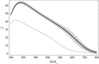
Equal-mass spin-aligned systems preserve a symmetry direction throughout their inspiral, insuring the $l=|m|=2$ modes dominate above higher (even) $l$ orders. Limiting attention to the $l=2$ subspace, the peak amplitude $\rho_{*,max}$ and source- and detector- orientation averaged amplitude $\bar{\rho}_{*}$ are related by

$$\rho_{*max}=\frac{5}{2}\bar{\rho}_{*}\qquad\text{l=2 only}$$ (20)

The $l>2$ modes in general and the $l=4$ modes in particular violate this relation: the signal power $\rho_{*,max}$ seen viewing along the symmetry axis increases linearly with $l>2$ amplitude; however, the orientation-averaged power $\bar{\rho}$ increases quadratically in the higher-harmonic amplitude (here, $l=4$). Keeping this distinction in mind, [Fig. 2] agree with Reisswig et al. (2009a) [their Fig. 6], who find that for lower-mass mergers $M\leq 500M_{\odot}$, $l=4$ modes are typically a $5-10\%$ correction in $\rho_{max}$ (depending on spin) to the individual signal-to-noise ratios $\rho_{max}$, but a much smaller correction to $\bar{\rho}$ and the ratio $\bar{\rho}/\bar{\rho}_{o}$. Moreover, as in all previous studies, aligned-spin waveforms appear to depend only extremely weakly if at all on the antisymmetric spin combination (${\boldsymbol{\chi}_{-}}$) Shoemaker et al. (2008), mostly through power-suppressed higher harmonics, suggesting ${\cal A}_{20}={\cal B}_{1020}\approx 0$. Additionally, as previous studies have shown, the orientation-averaged amplitude $\bar{\rho}$ increases monotonically with ${\boldsymbol{\chi}_{+}}\cdot z$. In terms of our expansion, its parameters must satisfy $\partial_{{{\boldsymbol{\chi}_{+}}\cdot{\mathbf{\hat{z}}}}}F>0$, or

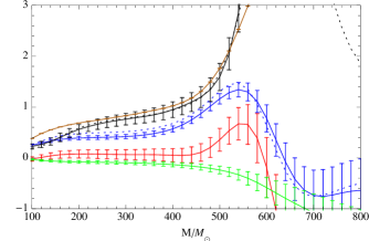
$${\cal X}_{1}+2{\cal X}_{2}({\boldsymbol{\chi}_{+}}\cdot{\mathbf{\hat{z}}})+3{\cal X}_{3}({\boldsymbol{\chi}_{+}}\cdot{\mathbf{\hat{z}}})^{2}>0\,.$$ (21)

Figure 3 provides our best estimates for the coefficient functions for $\bar{\rho}$ relevant to aligned spins, both employing all data (solid) and only $l=2$ aligned data (dashed); all satisfy this property. Though our general fit allows for small nonzero ${\cal A}_{20},{\cal B}_{1020},{\cal X}_{2}$, our equal-mass aligned spin data is well fit assuming these three parameters are exactly zero and the aligned-spin model consists of only ${\cal X}_{1,3}$ (dotted lines in Figure 3; for comparison, the fitting error $\delta F$ of this restricted model to aligned-only data is comparable to the fitting error shown in Figure 1 for a generic model to all data). Likewise, as our global fit error is often comparable to the change in $\bar{\rho}$ due to higher harmonics, particularly beyond $l=4$ for $M\leq 500M_{\odot}$, these harmonics can to a first approximation be neglected. Finally, for the mass range where $l=2$ emission dominates, the beampattern is extremely well approximated by the fiducial nonspinning values.

Figure 4: The relative significance of signal power due to different harmonics, shown for a nonspinning equal-mass binary seen by initial LIGO (top panel) and advanced LIGO (bottom panel), shown at an extraction radius $r=75$. The distances between the curves indicate $\bar{\rho}^{2}_{L}$, the signal power due to all $\rho$ harmonics. At each mass, $\bar{\rho}^{2}_{L}$ is normalized to the contribution from all $l\leq 4$ modes ($\bar{\rho}^{2}_{\leq 4}$) For advanced detectors, the quadrupole mode strongly dominates for most masses. Advanced detectors have much better low-frequency frequency sensitivity and particularly a much less steep low-frequency limit. On the contrary, low-mass detectors have a steep low-frequency boundary, strongly filtering out the $l=2$ mode once the final mass and spin lead to ringdown out of band.

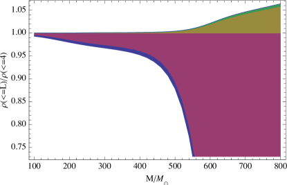
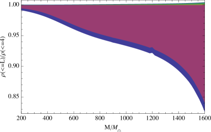
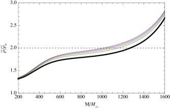
For a fixed bandpass detector, high mass favors higher harmonics, particularly when those harmonics are emitted from inspiral while the $l=2$ modes arise from the exponentially suppressed ringdown phase. For aligned binaries above $M\simeq 500M_{\odot}$, though the overall range drops, the $l=4$ harmonics provide an increasingly significant fraction of detectable power, even in the absence of spin; see Figure 4. As a result, based on the raw simulation data the beampattern correction for initial LIGO detectors evolves from $\bar{w}_{*}\approx 1.095$ at low mass (appropriate to $l=|m|=2$) down to a relatively isotropic $\bar{w}_{*}\approx 1.04$ at $M\simeq 600M_{\odot}$ during the transition between $l=2$ and $l=4$ beampatterns before eventually rising back at higher masses (i.e., approaching the value $1.085$ appropriate to $l=|m|=4$; see Table 3 and Appendix C). In principle, the process continues with higher harmonics; in practice, however, the detection volume is sufficiently small that their contribution to detection is negligible.

Though we estimate $\bar{\rho}$ as the nonspinning value $\bar{\rho}_{o}$ times a small “correction” $F$, at high mass and spin the raw numerical data requires extremely large $F$. Comparing Figure 2 with Figure 1, when the ratio of nonspinning to spinning $\bar{\rho}$ is large, our fit breaks down.

Convergence I: Extraction Radius

Our low-resolution large-radius grid zones do not retain enough information to permit adequately accurate waveform extraction for all harmonics. Therefore, unlike Reisswig et al. (2009a) who extract at $r=160M$ and particularly unlike extraction at ${\cal J}^{+}$ Reisswig et al. (2009b), we extract relatively close to the binary, at coordinate radii $r=40,50,60$ (and, when available, at $r=75$). As seen in Figure 5, finite extraction radius effects can compete with the small spin-dependent changes in $\bar{\rho}$.

For this reason, rather than adopt a single preferred extraction radius, we first extrapolate $\rho(M)$ to infinity, then fit to the extrapolated $\rho(M)$ data. Owing to instabilities in the extrapolation at high mass to $\bar{\rho}$ calculated using initial detector noise spectrum $S_{h}$, we do not trust our fit for extremely high masses $M\geq 500M_{\odot}$. On the contrary, for advanced detectors which lack such a steep low-frequency cutoff, our fitting procedure works well to proportionally higher masses; see Appendix A

Figure 5: For an equal-mass aligned-spin binary with $a_{1}=a_{2}=0.8$, estimates for $\bar{\rho}$ (top panel) and $\bar{\rho}/\bar{\rho}_{o}$ (bottom panel) seen by a single initial LIGO detector at $D=100\,{\rm Mpc}$ versus total binary mass $M$, based on waveforms extracted from our numerical merger simulations at coordinate extraction radii $r=40,50,60,75$ (blue, red, yellow, green), and (thick solid) linearly extrapolated in $1/r$ to $r\rightarrow\infty$. For high-mass mergers $M\geq 500M_{\odot}$, the aligned-spin range is much larger than the nonspinning range ($\bar{\rho}/\bar{\rho}_{o}>2$; compare to Figure 2). We anticipate both our extrapolation to large radius and our fit to perform poorly when the ratio $\bar{\rho}/\bar{\rho}_{o}$ is large.

Figure 6: For an equal-mass binary with $M=300M_{\odot}$ and generic spins, estimates for the fitting parameters ${\cal X}_{1,2,3}$ and ${\cal B}_{1020}$ to $\bar{\rho}/\bar{\rho}_{o}$, based on numerical waveforms extracted on spheres of radius $r=40,50,60$, shown versus $1/r$. Colors and symbols are associated as in Figure 3. This figure provides neither point error estimates nor extremely strong correlations between recovered parameters. Also shown at $1/r=0$ are the best-fit parameters to $\bar{\rho}/\bar{\rho}_{o}$ data that has been linearly extrapolated to $r\rightarrow\infty$ based on these radial slices as well as to the often-available $r=75$ slice. Finally, the light gray region indicates the range of extraction radii associated with our two lowest-resolution zones (i.e., between $r=80$ and $317$); to avoid introducing systematic error, we extrapolate over radii associated with a single grid zone.

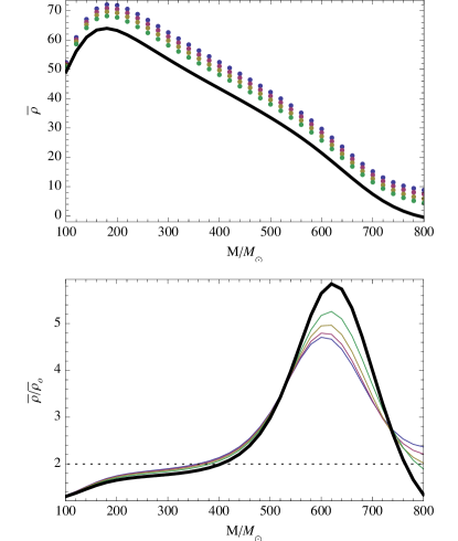
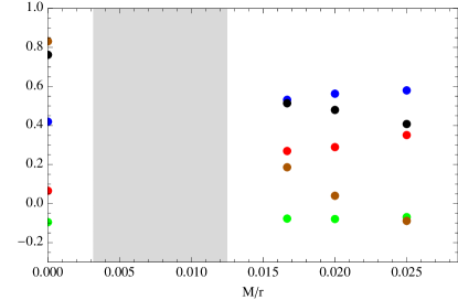
Figure 6 also demonstrates that specific coefficient values are sensitive to extrapolation, particularly the high-order (cubic) coefficients. This trend versus extraction radius demonstrates a key issue associated with any phenomenological fit: while we can present best-fit parameter estimates, these estimates are subject to strong correlations.

Despite uncertain and highly correlated fitting parameters, the best fit functions extracted from each extraction radius and from the radially extrapolated data are both extremely consistent with one another and with decreasing differences as $r$ increases. Specifically, performing Monte Carlo estimates of the $L^{2}$ difference between the finite-radius fits and the fit to extrapolated data, we find the set of $L^{2}$ functional differences $||F_{r}-F_{\infty}||$ (i) is consistent with being proportional to $1/r$ and (ii) at each radius is comparable to the semianalytic error estimate shown in Fig. 1.

V Selection biases for generic, comparable-mass mergers

Even well before the epochs considered here, binaries with generic spins precess, breaking symmetry and distributing power among other $l=2$ modes. The asymmetric merger process and ringdown favors exciting otherwise-suppressed higher harmonics (e.g., $l=3$), as well as the $l=4$ modes present even without spin. If the merger is in band, corresponding to masses $M\in[50,500]M_{\odot}$, higher harmonics contribute an increasing proportion of overall SNR, particularly at high spin; see, e.g., Fig. 2 in Shoemaker et al. (2008). As in the nonspinning case, if late stages of merger are detected, corresponding to masses $M\gtrsim 500M_{\odot}$ for initial and $M\gtrsim 1000M_{\odot}$ for advanced detectors, the beampattern can be significantly asymmetric. Unfortunately, though substantial beampattern asymmetries begin to occur at high mass and spin ($\bar{w}_{*}(M)$ varying), our fit to the angle-averaged power ($\bar{\rho}/\bar{\rho}_{o}$) is not accurate enough at these high masses to justify a detailed analysis. At lower mass, spin precession only weakly anisotropizes the beam. Comparing to our symmetry expansion [Eq. (II)], any (linear) leading-order spin-dependent corrections depend on only aligned spin components; the linear term is without loss of generality determined by simulations of aligned merging binaries. As the beampatterns from aligned merging binaries are dominated by $l=|m|=2$ emission, the beampattern correction factor for generic misaligned binaries $\bar{w}_{*}$ changes little from its nonspinning value. Though the beampattern changes shape substantially due to precession, its effective volume is nearly unchanged.

On the other hand, the average amplitude $\bar{\rho}$ varies substantially with spin magnitude and orientation. Well-known results for aligned spins illustrate the relative impact that spin orientations can produce. As a function of spin orientations relative to $\hat{L}$, the largest $\bar{\rho}$ occur with spins that are aligned with the orbit (${\boldsymbol{\chi}_{-}}=0;{\mathbf{S}}_{1,2}\propto{\mathbf{\hat{z}}}$); the smallest $\bar{\rho}$ occurs with spins that are antialigned with the orbit (${\boldsymbol{\chi}_{-}}=0;S_{1,2}\propto-{\mathbf{\hat{z}}}$); and $\bar{\rho}$ is essentially unchanged if the spins are mutually antialigned (${\boldsymbol{\chi}_{+}}=0$, both for $S_{1,2}\propto{\mathbf{\hat{z}}}$ and generally for all spin orientations ${\boldsymbol{\chi}_{-}}$). In fact, for these these intuitively obvious conditions to hold, the expansion parameters in Eq. (II) must satisfy the following conditions:

$${\cal A}_{20}\approx{\cal A}_{02} \approx 0$$

$${\cal X}_{1}\pm|{\boldsymbol{\chi}_{+}}|{\cal X}_{2}+\frac{3}{4}|{\boldsymbol{\chi}_{+}}|^{2}{\cal X}_{3} > \frac{{\cal B}_{1200}|{\boldsymbol{\chi}_{+}}|^{2}}{2}\pm|{\boldsymbol{\chi}_{+}}|{\cal X}_{02}$$

all of which our best-fit coefficients satisfy. As noted previously, because we included cubic-order terms, our fit for $\bar{\rho}$ is also consistent with $\bar{\rho}$ being a positive and monotonically increasing function of equal, aligned spins; see Eq. (21). More generally, for arbitrary spin orientations our fit is positive-definite for at least $M<500M_{\odot}$ and $|a_{1,2}|<0.8$, as well as for selected spin configurations at higher mass. As in the nonspinning case, however, our fit breaks down for binaries with large aligned spins and high mass, as in these regions the correction factor $F=\bar{\rho}/\bar{\rho}_{o}$ must be nearly $0$ (for spins mostly antialigned with the orbit) or much larger than unity (for component spins mostly aligned with the orbit).

Figures 3 and 8 provide our best-fit coefficients to the expansion of Eq. (II). These preferred values reproduce our best simulation resolutions, extrapolated to $r\rightarrow\infty$, including all available harmonics. Though the symmetry expansion of Eq. (II) permits more generic behavior with spin, our numerical results are well-fit with a far more restrictive form where only ${\cal X}_{1,2,3}$ and ${\cal X}_{02}$ are nonzero. As shown by the bottom panel in Figure 1, this fit performs well averaged over all simulations because our simulations mostly have $|a_{1,2}|\leq 0.6$ [Table 2], where cubic order corrections are still small. At the same time, the fit has more than enough parameters to explain the predominantly linear- and quadratic-order variation in $\bar{\rho}$ versus generic spin orientations; see for example Figure 7.

Figure 7: For a $M=200M_{\odot}$ binary, angle-averaged SNR ratio $F=\bar{\rho}/\bar{\rho}_{o}$ (points); our generic, unconstrained cubic-order fit $\hat{F}$ to all simulations (solid line); and a fit where only ${\cal X}_{1,2,3}$ and ${\cal X}_{02}$ can be nonzero (dashed lines). The data and fits are shown for spin magnitudes $a=0.4,0.6,0.8$ (green, blue, red, respectively) and spins ${\mathbf{S}}_{1}$ in the orbital plane (along the separation vector) and ${\mathbf{S}}_{2}$ tilted by angle $\theta$ away from ${\mathbf{\hat{z}}}$.

Figure 8: Fit coefficient functions ${\cal X}_{02},{\cal A}_{02},{\cal B}_{1200,1002}$ (black, red, blue,purple) and estimated least-squares fitting uncertainties $\Sigma_{kk}$ for the coefficients relevant to misaligned spin; compare with Figure 3. As in that figure, the large fitting errors ($\gtrsim 0.25$) on cubic-order terms (${\cal B}_{1200},{\cal B}_{1002}$) are not shown. Solid lines show a general fit including all harmonics and spins. The dotted black line corresponds to the value of ${\cal X}_{02}$ assuming a model where only it and ${\cal X}_{1,2,3}$ are nonzero.

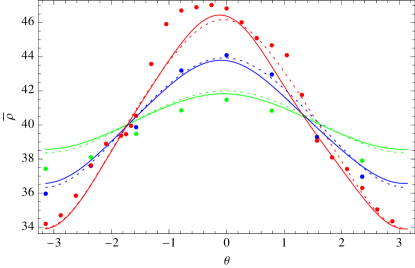
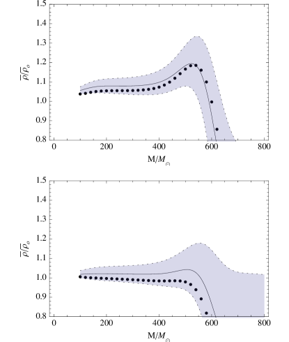
Blind test The first two simulations in Table 2, with random spins with $|a_{1}|=|a_{2}|=0.6$, were reserved as a blind test. As illustrated by Figure 9, for low masses $M\leq 500M_{\odot}$ our fit correctly recovers $\bar{\rho}/\bar{\rho}_{o}$ to within roughly the $1\sigma$ relative error ${\cal F}$, shown as the shaded region on this plot.

Figure 9: A plot of $F=\bar{\rho}/\bar{\rho}_{o}$ for the “blind test” spin configurations. Dots show the raw results from our numerical simulation; the curves and shaded region indicate results from our preferred fit.

VI Astrophysics

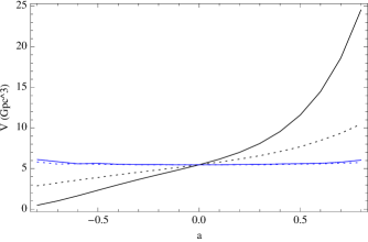
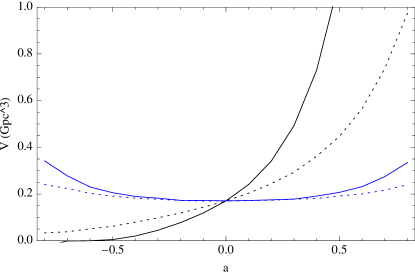
Using the fits provided in this paper, we can use Eq. (12) to determine the relative likelihood of observing different spin magnitudes and alignments, given a progenitor parameter distribution $p(\bar{\lambda})$. As expected from studies of aligned spins, ground-based gravitational wave detectors will be biased towards the detection of aligned and (to a lesser extent) large spins. For example, as seen in Figure 11 in the special case $M=200M_{\odot}$, populations of randomly oriented spins with identical magnitude $|a_{1}|=|a_{2}|=a$ are much less likely to be seen than a comparable population of spin-orbit aligned spins, and conversely for spin-orbit antialigned spins $a_{1}=a_{2}=-a{\mathbf{\hat{z}}}$. However, populations of binaries with random spins (dotted line in Figure 11) have comparable average detection volumes as nonspinning binaries, with detection volume increasing only $O(50\%)$ if spin magnitudes as large as $0.8$ are allowed, only marginally larger than fitting error in the detection volume. In other words, in a population of random spins, any pair of spin magnitudes are roughly likely to be observed, with only a slight bias towards larger spin magnitudes. Despite the much larger detection volume for aligned spins, a priori perfectly aligned and large spins should be rare, suppressing the bias towards high spin magnitude. For similar reasons, in any population of random spin orientations, large aligned spins occur rarely enough and the bias towards large spin is small enough (typically less than a factor 5) that the associated detected population will not be overabundant in tightly aligned spins unless the progenitor population is. For the purposes of illustration, suppose we assume any spin pair with both spins $S_{1,2}$ within $\pi/4$ of alignment with ${\mathbf{\hat{z}}}$ (i.e., $\hat{S}_{1,2}\cdot{\mathbf{\hat{z}}}>1/\sqrt{2}$) will be significantly amplified, independent of spin magnitude. Even in this unrealistically optimistic case, only $[(1-\cos\pi/4)/2]^{2}\simeq 2\%$ of all random progenitor spin orientations could be amplified.

All the properties described above and exhibited in Figure 11 can be understood analytically. For simplicity, let us adopt a fit with only ${\cal X}_{1,2,3}$ and ${\cal X}_{02}$ nonzero (dotted lines in Figures 3,8). The detection volume can be approximated to quadratic order as

$$V({\mathbf{S}}_{1},{\mathbf{S}}_{2}) \propto \bar{\rho}_{0}^{3}[1+3{\cal X}_{1}({\boldsymbol{\chi}_{+}}\cdot{\mathbf{\hat{z}}})+3({\cal X}_{1}^{2}+{\cal X}_{2})({\boldsymbol{\chi}_{+}}\cdot{\mathbf{\hat{z}}})^{2}$$ (22)

$$+ 3{\cal X}_{02}(P{\boldsymbol{\chi}_{+}})^{2}\,.+O(\chi^{3})]$$

Averaging the detection volume over all spin orientations (or any symmetric volumes in ${\mathbf{S}}_{1},{\mathbf{S}}_{2}$) eliminates terms of odd order, leaving only quadratic-order dependence on spin:

$$\left<V({\mathbf{S}}_{1},{\mathbf{S}}_{2})\right>_{\Omega} \propto \bar{\rho}_{0}^{3}[1+3({\cal X}_{1}^{2}+{\cal X}_{2})\left<({\boldsymbol{\chi}_{+}}\cdot{\mathbf{\hat{z}}})^{2}\right>_{\Omega}$$ (23)

$$+ 3{\cal X}_{02}\left<(P{\boldsymbol{\chi}_{+}})^{2}\right>_{\Omega}+O(\chi)^{4}]\,.$$

This expression reproduces the corresponding (blue dotted) curves in Fig. 11. Strictly speaking, our simulations and fit apply only to equal mass ratio. However, given symmetry considerations, the leading-order spin- and $\delta m/M$-dependent corrections to the detection volume must be quadratic in the asymmetric mass ratio times a quadratic function of spins. Our estimate therefore applies to many comparable-mass IMBH-IMBH mergers as well.

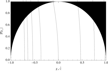
Some BH-BH binary populations have an intrinsic bias towards aligned spin, such as the products of binary evolution of extremely low-metallicity binary black holes. In these cases, spin-orbit misalignment encodes otherwise inaccessible information about the strength of supernova kicks on those very massive black holes. For an intrinsically aligned population, gravitational wave detectors are far more likely to observe large, tightly aligned spins. Figure 10 illustrates this effect using contours of the detection volume versus ${\boldsymbol{\chi}_{+}}\cdot{\mathbf{\hat{z}}}=(S_{1,z}+S_{2,z})/2$ (the aligned component of spin) and $(P{\boldsymbol{\chi}_{+}})^{2}$ (the perpendicular part of the symmetrized spin), adopting a fit with only ${\cal X}_{1,2,3}$ and ${\cal X}_{20}$ nonzero.

Figure 10: Contours of single-detector initial LIGO detection volume to an equal-mass $m_{1}=m_{2}=200M_{\odot}$ binary versus the symmetric spin ${\boldsymbol{\chi}_{+}}$, adopting a simple fit with only ${\cal X}_{1,2,3}$ and ${\cal X}_{02}$ nonzero. Contours are shown for $V=2^{n}V_{o}$ for $n=-4,-3\ldots 3$, increasing from left to right on the graph, where $V_{o}$ is the detection volume for zero spin. The shaded regions indicate physically unattainable ${\boldsymbol{\chi}_{+}}$ values (i.e., which must violate $|a_{1,2}|\leq 1$).

Below roughly $40\,{\rm Hz}$, the initial LIGO detector’s design sensitivity to merger waves ($O(f^{-7/3}/S_{h})$) decreases rapidly. Some mergers yield a final-state black hole whose ringdown frequency is comparable to this frequency. As a result, small changes in mass or spin lead to large changes in the volume to which these black holes can be seen. In particular, for black holes of fixed mass, this low-frequency cutoff produces a noticable bias towards large, aligned spins. Unfortunately, our fits to $\bar{\rho}$ degrade precisely where this selection bias becomes important. However, as seen in the bottom panel of Figure 11, the bias towards large spins is already apparent at $M=500M_{\odot}$. For example, at $a=0.8$, the blue solid line (randomly oriented spins) is twice as large as the nonspinning value, in contrast to only tens of percent higher at lower mass. At this and higher masses, the distance to which a nonspinning binary is visible can be substantially greater, up to a factor of $6$ or more near $M=600M_{\odot}$; see Fig. 5. This substantial increase in detection volume $\propto(\bar{\rho}/\bar{\rho}_{o})^{3}\simeq O(10-100)$ can partially compensate for the rarity with which random spin directions find themselves aligned. However, as this unusual selection bias for high spin operates only in a narrow mass and spin range and only for the initial detectors, we do not estimate this bias to an astrophysically relevant level of accuracy.

Figure 11: Detection volume for initial LIGO for BH-BH binary populations with $m_{1}=m_{2}=M/2=100M_{\odot}$ and different spin orientation and magnitude distributions: aligned, identical spins (black, solid); aligned spins independently distributed uniformly between $[0,a]$ or $[-|a|,0]$, if $a<0$ (black,dotted); randomly aligned spins with identical magnitude (blue, solid); and component spins independently drawn from a sphere of radius $a$ (blue, dashed). This figure provides only the single-detector beaming-uncorrected detection volume $V\equiv 4\pi(\bar{D})^{3}/3$ assuming a single-detector SNR threshold $\rho_{c}=8$; beaming increases the detection volume by roughly $(1.095)^{3}$. At low masses, far from the sharp initial LIGO low-frequency cutoff, all equal-mass binaries have a comparable detection volume. Bottom panel: as top panel, but now $m_{1}=m_{2}=250M_{\odot}$.

VII Conclusions

We have provided simple phenomenological fits to the average detection volume within which a merging equal-mass BH-BH binary with $M\in[100,500]M_{\odot}$ and arbitrary spins would produce a signal-to-noise ratio $\rho$ greater than a fixed detection threshold, for a single initial LIGO interferometer operating at design sensitivity. Comparable results for advanced LIGO are described in the Appendix. Though we describe fits for a single detector, our method also applies to arbitrary networks of identical detectors, adopting the universal angle-averaged power $\bar{\rho}$ combined with a suitably-modified (and network-topology-dependent) beaming correction factor $\bar{w}$. Our generic expression for the range is both surprisingly simple and accurate, involving at most 10 (=9+1) functions to reproduce the response to generic spin magnitudes and orientations to cubic order in the component spins. Moreover, we find an even simpler expression involving only four mass-dependent terms (${\cal X}_{1,2,3}$ and ${\cal X}_{02}$) also fits all our results. Though derived for equal mass ratio, symmetry considerations suggest unequal mass ratio corrections enter weakly, at higher order (in $\propto\delta m\,{\boldsymbol{\chi}_{-}}$). Our spin-dependent expressions for $\bar{\rho}/\bar{\rho}_{o}$ should therefore correctly estimate that ratio for all comparable-mass binaries. Finally, our method is easily extended to unequal mass: a three-parameter symmetry-constrained expansion of $\bar{\rho}/\bar{\rho}_{o}$ (in $\chi_{\pm}$ and $\delta m/M$) still has comparatively few parameters.

The dynamical processes that most likely produce merging BH-BH binaries at these masses likely guarantee random spin orientation Fregeau et al. (2006). Though gravitational wave detectors are far more sensitive to BH-BH binaries with aligned spins, we conclude that BH-BH populations with random spin orientations will rarely provide detections from tightly aligned, high-mass BH-BH binaries, under the assumption of optimal signal processing. Lacking the waveforms needed to perform optimal signal processing in the high-mass region, however, present-day all-sky gravitational wave searches conduct searches using approximate or hierarchical methods. Further study is needed to assess how strongly the search methodologies themselves introduce bias towards aligned spin.

Our fit suggests a surprising and astrophysically convenient conclusion: for $M\in[100,500]M_{\odot}$ for initial LIGO and over $M\in[200,1600]M_{\odot}$ for advanced LIGO, the population-averaged detection volume for binaries with random spin directions and an arbitrary spin magnitude distribution and $a_{1,2}<0.8$ is nearly identical (within tens of percent, comparable to the Poisson error in 10 detections) to the detection volume for nonspinning binaries of comparable mass. On the contrary, detectors like initial LIGO which have both a shallow optimally sensitive region combined with a very steep low frequency cutoffs will be noticably more likely to recover large aligned spins from a random spin population, albeit only for the very highest masses and spins to which the detector is sensitive ($M>500M_{\odot}$ for initial LIGO).

Conversely, our analysis implies that the detected population of high-mass binaries with a given (optimally filtered) SNR $\rho$ will be distributed uniformly over spin orientations, to the extent that their formation processes produce them. Our study therefore reaffirms the urgent need for models for the merger waveforms from generic spinning merging binaries.

At present, our fit breaks down at very high mass, empirically when $(\bar{\rho}/\bar{\rho}_{o}-1)$ is of order unity. Several avenues of improvement could make the fit more stable: fitting to a logarithm $\ln\bar{\rho}/\bar{\rho}_{o}$, or even using similarity transformations to rescale $\bar{\rho}(M)$ to different spin geometries (e.g., changing the mass and amplitude scale using the ringdown frequency of the post-merger BH). We have also not compared our fitting parameters with comparable coefficients for better-understood low-mass binaries (e.g., those undergoing simple precession), which can be estimated analytically and numerically. We will address these refinements in a future paper.

For simplicity, our analysis is expressed in terms of matched filtering and a fixed SNR detection threshold. Whether due to incomplete signal models, inefficiencies in template placement, or the lack of a signal model altogether, realistic searches cannot identify all available signal power. Additionally, whether from higher mass or antialigned spin, waveforms of short duration are more easily confused with nongaussian detector noise and require a significantly higher detection threshold. Though a significant technical challenge, the search- and detector-dependent effective detection threshold versus binary parameters $\rho_{c}(\lambda)$ that incorporates both mismatch and noise effects can also be tabulated. For example, for low mass binaries the mismatch between nonspinning search templates and precessing, spinning waveforms has been tabulated; see Brown et al. (in preparation). Combined with our fit to the intrinsic available detection volume, a “detector sensitivity” fit could efficiently communicate an adequately-accurate representation of the parameter-dependent detection volume of real high-mass searches.

To summarize, we have provided the first phenomenological fit to the spin-dependent detection horizon for generic spin magnitudes, spin orientations, and (equal) component masses $M\in[100,800M_{\odot}]$. We have shown that to leading order spin effects average out of the detection volume. For example, the rate at which IMBH-IMBH mergers will be detected is directly proportional to this volume. All previous estimates for the IMBH-IMBH detection rate estimated this volume assuming minimal or occasionally aligned component spins Gair et al. (2009); Amaro-Seoane and Santamaria (2009); Mandel et al. (2009) and therefore should be nearly unchanged even with spin included.

Appendix A Selection biases of individual advanced detectors

For pedagogical reasons, in the text we described our procedure estimating selection biases versus spin in the context of a single detector design (initial LIGO). In this appendix we provide a similar discussion for advanced and third-generation detectors, specifically the benchmark advanced LIGO Harry and the LIGO Scientific Collaboration (2010) and Einstein Telescope Sathyaprakash and et. al (2009) designs. These instruments’ sensitivity is great enough that, even without detections, their upper limits rule out otherwise astrophysically plausible progenitor models. We particularly emphasize how these detectors superior low-frequency sensitivity leads to much more accurate fits, over a broader range of masses.

For simplicity, despite both detectors’ cosmologically significant range, we perform all calculations in terms of the luminosity distance and redshifted mass – effectively as if in a flat universe. Though our fits reproduce $\bar{\rho}/\bar{\rho}_{o}$ to several percent, and though the reader can invert any particular line of sight to that accuracy, we have not included all information needed to completely reconstruct the selection bias versus mass and spin. At these distances, the detection volume is no longer proportional to a simple cubic moment of the beampattern function; see for example the appendix of O’Shaughnessy et al. (2009) for a comparable calculation at low mass. Though we anticipate the comoving volume swept out by the past detection light cone will not depend sensitively on the details of its truncation at large redshift, we have not thoroughly explored the errors our neglect of these effects introduces.

By adopting luminosity distance and redshifted mass as parameters, each result in this section is directly comparable to a corresponding prediction for initial detectors. However, because advanced detectors have peak sensitivity at roughly $2\times$ lower frequency, the response of initial detectors of mass $M$ contains comparable waveform content as and is best compared to the response of advanced detectors of mass $2M$. For example, the low-mass limit for initial LIGO is roughly $100M_{\odot}$ for initial and $200M_{\odot}$ for advanced detectors.

A.1 Average signal power versus binary spins

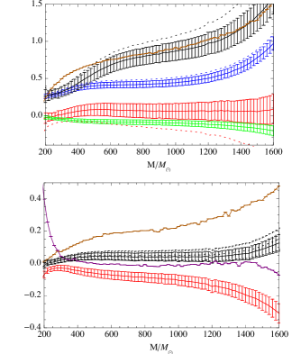
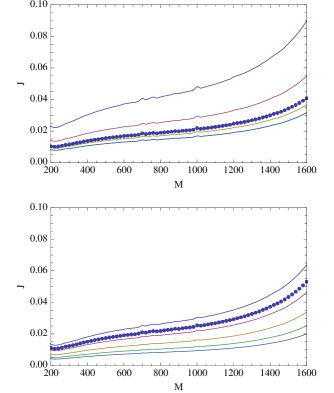
Unlike the results from initial detectors, the data for $\bar{\rho}/\bar{\rho}_{o}$ exhibits relatively weak dependence on spin for all masses. As a result, a fit to the numerical data performs well, both reproducing the data (Fig. 13) and producing well-determined fitting coefficients (Fig. 12) over the entire range of plausible masses $M\in[200,1600]M_{\odot}$. Aside from a difference in scale, however, the fit exhibits properties comparable to the low-mass fit ($M<500M_{\odot}$) to initial LIGO $\bar{\rho}$. Notably, (i) the fit is dominated by aligned spin coefficients, with few resolved corrections involving perpendicular spins; (ii) it depends only weakly on antisymmetric spin ${\boldsymbol{\chi}_{-}}$; (iii) it satisfies all sanity conditions, such as increasing monotonically with aligned spin and attaining a local extrema versus orientation when equal-magnitude spins aligned and antialigned; and finally (iv) higher harmonics $l>3$ only weakly change the best-fit coefficient functions $y_{\alpha}$, mostly at the highest masses. Also as in the low-mass fit, the fitting coefficients are strongly correlated. Ill-constrained high-order coefficients like ${\cal B}_{1020}$ are sensitive to numerical issues, such as extrapolation to large radius. Most differences between the performance of initial and advanced detectors is directly attributable to their low-frequency response: advanced detectors generally lack an abrupt transition from peak to low-frequency sensitivity. Without a strong preferred frequency these detectors must have at best a weak bias towards recovering the largest and most tightly aligned spins; compare Section IV. Furthermore, as discussed by example in the Appendix B, because of the nearly power-law low-frequency response of the detector noise power spectrum, the fitting coefficients are nearly constant, independent of mass.

Figure 12: Coefficients of fit to the ratio $\bar{\rho}/\bar{\rho}_{o}$ for single design-sensitivity advanced LIGO detector; compare the top panel to Figures 8 and 8. The advanced LIGO detector design will be sensitive to lower characteristic frequencies [$O(40\,{\rm Hz})$ vs $O(100\,{\rm Hz})$ for the initial detector]. For this reason, we provide fits over a more limited mass range: only above $200M_{\odot}$ will our short waveforms start their inspiral well before they enter band.

Figure 13: Expected $1\sigma$ error ${\cal F}$ in an unconstrained fit to $F=\bar{\rho}/\bar{\rho}_{o}$ for advanced LIGO detectors, for spin magnitudes $|a_{1}|,|a_{2}|$ limited to below unity (blue; largest); below $0.8$ (red); and below $0.6,0.4$ and $0.2$ (similar curves near bottom). Also shown (points) are the least-squares errors $\delta F$ between our fit $\hat{F}$ and the simulated NR data. Top panel shows standard; bottom panel shows error of restricted model. Because of its broader bandpass, the advanced detector range is more accurately modeled by our expansion; compare Fig. 1.

Figure 14: For an equal-mass aligned spin binary with $a_{1}=a_{2}=0.8$, estimates for $\bar{\rho}/\bar{\rho}_{o}$ seen by a single advanced LIGO detector at $D=100\,{\rm Mpc}$ versus total binary mass $M$, based on waveforms extracted from our numerical merger simulations at coordinate extraction radii $r=40,50,60,75$ (blue, red, yellow, green) and (thick solid) linearly extrapolated in $1/r$ to $r\rightarrow\infty$.

Figure 15: Coefficients of fit to the ratio $\bar{\rho}/\bar{\rho}_{o}$ for single design-sensitivity Einstein Telescope; compare the top panel to Figures 8 and 8.

Appendix B Analytic estimates for expansion coefficients

As seen in the text, the relative detection volume for different spinning binaries is largely determined by the angle-averaged SNR $\bar{\rho}$. At both very low and very high mass, the leading-order dependence of the angle-averaged SNR on spin orientation can be calculated, particularly by adopting high-symmetry configurations such as spin-aligned binaries to better isolate relevant terms. For example, at very low mass the aligned spin coefficients such as ${\cal X}_{1,2,3}$ follow from the well-known stationary-phase Fourier transform of the 2.5-PN-accurate inspiral waveform for spinning, aligned binaries. Adopting the restricted Newtonian amplitude at all frequencies and expanding $\sqrt{d\omega/dt}$ in the denominator of the stationary-phase Fourier transform, the leading order change in SNR with spin follows approximately from

$${\cal X}_{1} \approx \frac{47}{24}M\pi\frac{J(4/3)}{J(7/3)}$$ (24)

$${}J(q) = \int_{0}^{\infty}\frac{f^{-q}}{S_{h}}$$ (25)

On the other extreme, only the late-stage ringdown of very high-mass spinning binaries will fall into our detectors’ sensitive band. Qualitatively, ringdown emission produces an SNR limited by the detector frequency and total amount of emitted power. Progenitor black hole spins will change the total amount of emitted energy and, critically, the final hole ringdown frequency. Assuming ringdown waves are nearly monochromatic and contain a proportion of the total emitted energy, the high-mass SNR can be roughly estimated by the nonspinning amplitude at that mass times an ad-hoc ringdown correction factor:

$$\bar{\rho} = \bar{\rho}_{o}\frac{\sqrt{(M_{f}-M)/(M_{f,o}-M)}}{\sqrt{S_{h}(f_{rd})/S_{h}(f_{rd,o})}}$$ (26)

where $f_{rd}(M_{f},a_{f})\approx[1-0.63(1-a_{f})^{3/10}]/2\pi M_{f}$ is the ringdown frequency of the final hole of mass $M_{f}$ and spin $a_{f}$ and where $M_{f},a_{f}$ are known expressions of the progenitor masses and spins. If for simplicity we further retain only $\chi_{+,z}$ spin dependence, then we find an expression for ${\cal X}_{1}$ in terms of the detector’s noise power spectrum $S_{h}$:

$$\bar{\rho}/\bar{\rho}_{o} = 1+\chi_{+,z}\left[0.0888-0.0706\frac{d\ln S_{h}}{Mdf}_{f_{rd}}\right]+\ldots$$ (27)

$$= 1+\chi_{+,z}\left[0.0888+0.0706\frac{p\pi(M_{f}/M)}{(f_{rd,0}M_{f})}\right]$$

where in the last term we assume the detector’s low frequency noise is a pure power law ($S_{h}(f)\propto f^{-p}$). The second term is a positive-definite constant, independent of mass and depending predominantly on the physics of BH mergers; the detector influences this estimate for $\bar{\rho}$ only through the low-frequency noise exponent $p$. Though not a quantitatively precise model for $\bar{\rho}$ – the fits described in the paper are required to estimate the detection volume to astrophysically-relevant accuracy – this simple ringdown-dominated signal model illustrates why ${\cal X}_{1}$ must vary relatively little between detector designs. Our estimate also identifies changes in $d\ln S_{h}/d\ln f(f=f_{rd}(M))$ as key points where ${\cal X}_{1}(M)$ should change significantly.

Appendix C Detection volume for networks

In the text, we estimated the detection volume to which a single perpendicular-arm interferometer with a fixed detection threshold could recover a source of unknown sky location. We expressed this simple measure of sensitivity in terms of two factors ($\bar{\rho}_{*},w_{*}$) . Real searches employ multiple detectors, providing sensitivity to both polarizations nearly everywhere on the sky. Their relative orientations determine a sky position- and polarization- dependent sensitivity. Unfortunately, real searches also have detectors with different (and time-dependent) noise power; a network whose nodes are not always active; and of course beampatterns that are highly nonuniform. A completely realistic treatment of multidetector search sensitivity adopting realistic search strategies and thresholds is beyond the scope of this paper.

Though necessarily incomplete, the analytic estimates of idealized detector performance nonetheless allow us to quickly understand the dominant qualitative effects spin might have on the detection volume, such as Fig. 11. Similar analytic estimates for idealized networks can be constructed, albeit depending on network topology. For coherent multidetector searches with identical detectors, their sensitivity along any direction is described in general by a 2x2 Hermetian matrix for each sky position Cutler and Flanagan (1994); for brevity, we will limit attention to this case henceforth. This orientation- and polarization-dependent sensitivity implies the true beampattern function $w$ of both source- and sky position- orientations becomes very complex in general, particularly when multiple harmonics with different shapes contribute to the overall response. Nonetheless, there are three physically interesting approximations where the average amplitude and beampattern are tractable:

• Single detector (used in text): Sensitivity is characterized by an angle-averaged SNR $\bar{\rho}_{*}$ [Eq. (II)]; a beampattern function $w_{*}=\rho/\bar{\rho}_{*}$ of sky position and source orientation; and a beampattern effective radius $\bar{w}_{*}=\left<w_{*}^{3}\right>^{1/3}$ [Eq. (13)], averaged over all orientations.

  To provide a concrete example, consider the case of a binary dominated by $l=|m|=2$ emission, viewed by a single interferometer. Since the beampattern $w$ versus all angles is known analytically [e.g., Eq. (2) in O’Shaughnessy et al. (2009)], the amplitude $\rho$ versus orientation is completely determined by the optimally-oriented amplitude $\rho_{\rm*,max}$, or equivalently by the “horizon distance” $D_{\rm h}$ at which $\rho_{max}=\rho_{c}$.

  $$\bar{\rho}_{*} = \rho_{*,max}\frac{2}{5}=\rho_{c}\frac{2}{5}\frac{D_{h}}{D}$$ (28)

  $$\bar{D}_{*} = D_{h}2/5$$ (29)

  $$\bar{w}_{*} = 1.095$$ (30)

  Alternatively, the sensitivity of the interferometer can be characterized by source-orientation-averaged effective detection volume, or, to use similar units, the volume-averaged distance $D_{\rm v}$. The above expressions allow us to express familiar relationship between $D_{\rm v}$ and $D_{\rm h}$ O’Shaughnessy et al. (2009) in terms of the single-detector beampattern correction factor $\bar{w}_{*}$:

  $$D_{v} = D_{h}2\bar{w}_{*}/5\approx D_{h}/(2.26)$$ (31)

• Isotropic network, equal polarization sensitivity : At the other extreme from a single-detector network is the ideal case: a network with equal sensitivity to both polarizations in all directions. Assuming searches for this ideal network are carried out by matched filtering, its network sensitivity is characterized by an angle-averaged two-polarization network SNR $\bar{\rho}=\bar{\rho}_{*}\sqrt{5}$ [Eq. (5); see Cutler and Flanagan (1994)]; a beampattern function $w=\rho/\bar{\rho}$; and a source-orientation-averaged moment

  $$\bar{w}= = \frac{[\int\frac{d\Omega_{n}}{4\pi}w({\mathbf{\hat{n}}})^{3}]^{1/3}}{\left<w^{2}\right>^{2/3}}\;.$$ (32)

  where, because the detector has equal sensitivity to both polarizations, the orientation average needs to be conducted only over all emission directions ${\mathbf{\hat{n}}}$.

• Isotropic network, single polarization sensitivity: In between these two extremes is an isotropic network with sensitivity to only one polarization at each sky position. For example, the three-site LIGO-Virgo network is primarily sensitive to one polarization for each sky position. Using a subscript $0$ to denote this class of detector, the the beampattern function can be similarly defined as a suitable average over emission direction ${\mathbf{\hat{n}}}$ and polarization angle $\psi$:

  $$\bar{w}_{0} = \left<w_{0}^{3}\right>^{1/3}/\left<w_{0}^{2}\right>$$ (33)

  By symmetry, the orientation-averaged signal power must be precisely half that of a network sensitive to two polarizations, so $\bar{\rho}_{0}=\bar{\rho}/\sqrt{2}$.

To illustrate the beaming-induced differences in detection volume between these different network topologies, in Table 3 we tabulate the beaming correction factors when a particular multipolar mode dominates emission ($l=|m|$). All are nearly unity; all depend weakly on $l$, for a given detector topology. Additionally, the beaming correction factors have a universal hierarchy: $\bar{w}_{o}>\bar{w}_{*}>\bar{w}$. Obviously the idealized two-polarization-sensitive isotropic network has the most symmetric beampattern, least sensitive to host orientation and polarization content. Conversely, an isotropic network sensitive to one polarization is usually the most sensitive to unfortunately oriented (polarized) sources.

l	$\bar{w}_{o}$	$\bar{w}_{*}$	$\bar{w}$
2	1.11661	1.09664	1.05065
4	1.10614	1.08541	1.0408
6	1.15301	1.12961	1.08489

Table 3: Beaming correction factors when a single $l=|m|$ mode dominates emission. In this table, $\bar{w}_{*}$ times $1/\sqrt{5}$ characterizes the radius of the detection volume associated with an all-sky search for a single source by a single interferometer; $\bar{w}$ (without additional factors) refers to a comparable search by a network with isotropic sensitivity to both polarizations; and $\bar{w}_{o}$ refers to a network with isotropic sensitivity to a single polarization.

References

- Acernese et al. (2006) F. Acernese, P. Amico, M. Alshourbagy, F. Antonucci, S. Aoudia, S. Avino, D. Babusci, G. Ballardin, F. Barone, L. Barsotti, et al., Classical and Quantum Gravity 23, 635 (2006).
- Abbott et al. (2003) (The LIGO Scientific Collaboration) Abbott et al. (The LIGO Scientific Collaboration), (gr-qc/0308043) (2003), URL http://xxx.lanl.gov/abs/gr-qc/0308043.
- Shoemaker and the LIGO Scientific Collaboration (2009) D. Shoemaker and the LIGO Scientific Collaboration (2009), URL https://dcc.ligo.org/cgi-bin/DocDB/ShowDocument?docid=2974.
- O’Shaughnessy et al. (2009) R. O’Shaughnessy, V. Kalogera, and K. Belcynski, (arXiv:0908.3635) Submitted to ApJ (2009), eprint 0908.3635.
- Belczynski et al. (2010) K. Belczynski, M. Dominik, T. Bulik, R. O’Shaughnessy, C. L. Fryer, and D. E. Holz, (arXiv:1004.0386) (2010), eprint 1004.0386.
- O’Shaughnessy et al. (2007) R. O’Shaughnessy, R. O’Leary, and F. A. Rasio, Phys. Rev. D 76, 061504 (2007), eprint 0701887.
- Sadowski et al. (2008) A. Sadowski, K. Belczynski, T. Bulik, N. Ivanova, F. A. Rasio, and R. O’Shaughnessy, Astrophys. J. 676, 1162 (2008).
- Banerjee et al. (2010) S. Banerjee, H. Baumgardt, and P. Kroupa, MNRAS 402, 371 (2010), eprint 0910.3954.
- Fregeau et al. (2006) J. M. Fregeau, S. L. Larson, M. C. Miller, R. O’Shaughnessy, and F. A. Rasio, Astrophys. J. 646, L135 (2006), URL http://xxx.lanl.gov/abs/astro-ph/0605732.
- Lousto et al. (2010) C. O. Lousto, H. Nakano, Y. Zlochower, and M. Campanelli, Phys. Rev. D 81, 084023 (2010), eprint 0910.3197.
- Campanelli et al. (2009) M. Campanelli, C. O. Lousto, H. Nakano, and Y. Zlochower, Phys. Rev. D 79, 084010 (2009), eprint 0808.0713.
- Szilágyi et al. (2009) B. Szilágyi, L. Lindblom, and M. A. Scheel, Phys. Rev. D 80, 124010 (2009), eprint 0909.3557.
- Campanelli et al. (2010) M. Campanelli, C. O. Lousto, B. C. Mundim, H. Nakano, Y. Zlochower, and H. Bischof, Classical and Quantum Gravity 27, 084034 (2010), eprint 1001.3834.
- Rezzolla (2009) L. Rezzolla, Classical and Quantum Gravity 26, 094023 (2009), eprint 0812.2325.
- Barausse and Rezzolla (2009) E. Barausse and L. Rezzolla, ApJL 704, L40 (2009), eprint 0904.2577.
- Marronetti et al. (2008) P. Marronetti, W. Tichy, B. Brügmann, J. González, and U. Sperhake, Phys. Rev. D 77, 064010 (2008), eprint 0709.2160.
- Kesden et al. (2010) M. Kesden, U. Sperhake, and E. Berti, Phys. Rev. D 81, 084054 (2010), eprint 1002.2643.
- Ajith et al. (2009) P. Ajith, M. Hannam, S. Husa, Y. Chen, B. Bruegmann, N. Dorband, D. Mueller, F. Ohme, D. Pollney, C. Reisswig, et al., (arXiv:0909.2867) (2009), eprint 0909.2867.
- Reisswig et al. (2009a) C. Reisswig, S. Husa, L. Rezzolla, E. N. Dorband, D. Pollney, and J. Seiler, Phys. Rev. D 80, 124026 (2009a), eprint 0907.0462.
- Pan et al. (2010) Y. Pan, A. Buonanno, L. T. Buchman, T. Chu, L. E. Kidder, H. P. Pfeiffer, and M. A. Scheel, Phys. Rev. D 81, 084041 (2010), eprint 0912.3466.
- Flanagan and Hughes (1998) É. É. Flanagan and S. A. Hughes, Phys. Rev. D 57, 4535 (1998).
- Boyle and Kesden (2008) L. Boyle and M. Kesden, Phys. Rev. D 78, 024017 (2008).
- Boyle et al. (2007) L. Boyle, M. Kesden, and S. Nissanke, (arXiv:0709.0299) (2007), eprint 0709.0299.
- Rezzolla et al. (2008a) L. Rezzolla, E. Barausse, E. N. Dorband, D. Pollney, C. Reisswig, J. Seiler, and S. Husa, Phys. Rev. D 78, 044002 (2008a).
- Rezzolla et al. (2008b) L. Rezzolla, P. Diener, E. N. Dorband, D. Pollney, C. Reisswig, E. Schnetter, and J. Seiler, ApJL 674, L29 (2008b).
- Baker et al. (2008a) J. G. Baker, W. D. Boggs, J. Centrella, B. J. Kelly, S. T. McWilliams, M. C. Miller, and J. R. van Meter, ArXiv e-prints 802 (2008a).
- Abadie et al. (2010) (The LIGO Scientific Collaboration) B. Abadie et al. (The LIGO Scientific Collaboration), (arXiv:1003.2481) (2010), eprint 1003.2481.
- Herrmann et al. (2007) F. Herrmann, I. Hinder, D. M. Shoemaker, P. Laguna, and R. A. Matzner, Phys. Rev. D76, 084032 (2007), eprint 0706.2541.
- Herrmann et al. (2007) F. Herrmann, I. Hinder, D. Shoemaker, and P. Laguna, Classical and Quantum Gravity 24, S33 (2007), eprint arXiv:gr-qc/0601026.
- Herrmann et al. (2007) F. Herrmann, I. Hinder, D. Shoemaker, P. Laguna, and R. A. Matzner, Astrophys. J. 661, 430 (2007), eprint gr-qc/0701143.
- Hinder et al. (2008a) I. Hinder, B. Vaishnav, F. Herrmann, D. Shoemaker, and P. Laguna, Phys. Rev. D77, 081502 (2008a), eprint 0710.5167.
- Healy et al. (2009a) J. Healy et al., Phys. Rev. Lett. 102, 041101 (2009a), eprint 0807.3292.
- Hinder et al. (2008b) I. Hinder, F. Herrmann, P. Laguna, and D. Shoemaker, arxiv:0806.1037 (2008b), eprint 0806.1037.
- Healy et al. (2009b) J. Healy, J. Levin, and D. Shoemaker, Phys. Rev. Lett. 103, 131101 (2009b), eprint 0907.0671.
- Healy et al. (2010) J. Healy, P. Laguna, R. A. Matzner, and D. M. Shoemaker, Phys. Rev. D81, 081501 (2010), eprint 0905.3914.
- Bode et al. (2010) T. Bode, R. Haas, T. Bogdanovic, P. Laguna, and D. Shoemaker, Astrophys. J. 715, 1117 (2010), eprint 0912.0087.
- Schnetter et al. (2004) E. Schnetter, S. H. Hawley, and I. Hawke, Class. Quant. Grav. 21, 1465 (2004).
-
(38)
cactus-web, cactus Computational Toolkit home page:
http://www.cactuscode.org. - Husa et al. (2006) S. Husa, I. Hinder, and C. Lechner, Computer Physics Communications 174, 983 (2006).
- Baker et al. (2007) J. G. Baker, S. T. McWilliams, J. R. v. Meter, J. Centrella, D. Choi, B. J. Kelly, and M. Koppitz, Phys. Rev. D 75, 124024 (2007), URL http://xxx.lanl.gov/abs/gr-qc/0612117.
- Scheel et al. (2008) M. A. Scheel, M. Boyle, T. Chu, L. E. Kidder, K. D. Matthews, and H. P. Pfeiffer, ArXiv e-prints (2008).
- Baker et al. (2008b) J. G. Baker, W. D. Boggs, J. Centrella, B. J. Kelly, S. T. McWilliams, and J. R. van Meter, Phys. Rev. D 78, 044046 (2008b).
- Vaishnav et al. (2007) B. Vaishnav, I. Hinder, F. Herrmann, and D. Shoemaker, Phys. Rev. D 76, 084020 (2007).
- Shoemaker et al. (2008) D. Shoemaker, B. Vaishnav, I. Hinder, and F. Herrmann, Classical and Quantum Gravity 25, 114047 (2008).
- Ajith et al. (2007) P. Ajith, S. Babak, Y. Chen, M. Hewitson, B. Krishnan, J. T. Whelan, B. Brügmann, P. Diener, J. Gonzalez, M. Hannam, et al., Classical and Quantum Gravity 24, 689 (2007), eprint 0704.3764.
- Ajith et al. (2008) P. Ajith, S. Babak, Y. Chen, M. Hewitson, B. Krishnan, A. M. Sintes, J. T. Whelan, B. Brügmann, P. Diener, N. Dorband, et al., Phys. Rev. D 77, 104017 (2008).
- Sturani et al. (2010) R. Sturani, S. Fischetti, L. Cadonati, G. M. Guidi, J. Healy, D. Shoemaker, and A. Viceré, ArXiv e-prints (2010), eprint 1005.0551.
- Reisswig et al. (2009b) C. Reisswig, N. T. Bishop, D. Pollney, and B. Szilagyi, (arXiv:0912.1285) (2009b), URL http://xxx.lanl.gov/abs/arXiv:0912.1285.
- Amaro-Seoane and Santamaria (2009) P. Amaro-Seoane and L. Santamaria, ArXiv e-prints (2009).
- Mandel et al. (2009) I. Mandel, J. R. Gair, and M. C. Miller, ArXiv e-prints (2009).
- Gair et al. (2009) J. R. Gair, I. Mandel, M. C. Miller, and M. Volonteri, (arXiv:0907.5450) (2009), URL http://xxx.lanl.gov/abs/arXiv:0907.5450.
- Harry and the LIGO Scientific Collaboration (2010) G. M. Harry and the LIGO Scientific Collaboration, Classical and Quantum Gravity 27, 084006 (2010).
- Sathyaprakash and et. al (2009) B. Sathyaprakash and et. al (2009), URL https://workarea.et-gw.eu/et/WG4-Astrophysics/visdoc/.
- Cutler and Flanagan (1994) C. Cutler and E. Flanagan, Phys. Rev. D 49, 2658 (1994), eprint gr-qc/9402014.