The Tully-Fisher relations of early-type spiral and S0 galaxies

Abstract

We demonstrate that the comparison of Tully-Fisher relations (TFRs) derived from global H i line widths to TFRs derived from the circular velocity profiles of dynamical models (or stellar kinematic observations corrected for asymmetric drift) is vulnerable to systematic and uncertain biases introduced by the different measures of rotation used. We therefore argue that to constrain the relative locations of the TFRs of spiral and S0 galaxies, the same tracer and measure must be used for both samples. Using detailed near-infrared imaging and the circular velocities of axisymmetric Jeans models of 14 nearby edge-on Sa–Sb spirals and 14 nearby edge-on S0s drawn from a range of environments, we find that S0s lie on a TFR with the same slope as the spirals, but are on average $0.53\pm 0.15$ mag fainter at $K_{S}$-band at a given rotational velocity. This is a significantly smaller offset than that measured in earlier studies of the S0 TFR, which we attribute to our elimination of the bias associated with using different rotation measures and our use of earlier type spirals as a reference. Since our measurement of the offset avoids systematic biases, it should be preferred to previous estimates. A spiral stellar population in which star formation is truncated would take $\approx 1$ Gyr to fade by 0.53 mag at $K_{S}$-band. If S0s are the products of a simple truncation of star formation in spirals, then this finding is difficult to reconcile with the observed evolution of the spiral/S0 fraction with redshift. Recent star formation could explain the observed lack of fading in S0s, but the offset of the S0 TFR persists as a function of both stellar and dynamical mass. We show that the offset of the S0 TFR could therefore be explained by a systematic difference between the total mass distributions of S0s and spirals, in the sense that S0s need to be smaller or more concentrated than spirals.

1 Introduction

Both early- and late-type galaxies follow scaling relations. In the case of elliptical galaxies, the radii, velocity dispersions and luminosities lie on a Fundamental Plane (Djorgovski & Davis, 1987; Dressler et al., 1987). The luminosities of disc galaxies scale with their sizes (Freeman, 1970), rotation speeds (Tully & Fisher, 1977) and colours (Tully et al., 1982). The existence, scatter and evolution of these scaling relations provides powerful constraints for models of galaxy formation and evolution.

In this work we concentrate on the Tully-Fisher relation (TFR), first discovered by Tully & Fisher (1977). In its original form, the TFR relates the global H i line widths of disc galaxies to their total luminosities. The line width of a rotationally-supported galaxy is a measure of the difference between the maximum rotation velocities of the approaching and receding sides. A galaxy’s luminosity is related to the mass of its luminous component (and the evolutionary state of the stellar populations). The observed correlation between global line widths and luminosities is therefore a manifestation of a more general connection between galaxy masses and rotational velocities. A correlation is of course expected for gravitationally bound systems in which the mass distribution is dominated by luminous matter.

Empirically, the correlation is tight enough to allow the TFR to be inverted and used to determine distances (e.g. Sakai et al., 2000; Tully & Pierce, 2000, hereafter TP00), but systematic variations of the residuals can arguably be used to infer the properties of dark haloes (Courteau & Rix, 1999). Efforts to simultaneously reproduce the zero-point of the TFR and the galaxy luminosity function with semi-analytical models of galaxy formation may reveal further information on the role of the halo, the importance of feedback and the evolution of the stellar populations (e.g. Baugh, 2006; Dutton et al., 2007). It is therefore clear that investigating variations of the local TFR with galaxy luminosity, size, type and other parameters should provide valuable insight into the growth of luminous structures in the Universe.

There are systematic variations in the slope, intercept and scatter of the TFR as a function of galaxy type. Roberts (1978) and Rubin et al. (1985) found that Sa spirals are fainter than Scs for a given rotational velocity at optical wavelengths. At least some of this difference has been attributed to variation in the shape of rotation curves related to the bulge-to-disc ratio (Verheijen, 2001; Noordermeer & Verheijen, 2007). The difference is much smaller in the near-infrared (Aaronson & Mould, 1983; Peletier & Willner, 1993). This has been taken as evidence that the discrepancy at optical wavelengths is at least partially due to the effects of recent star formation on the luminosity, which is reduced in the near-infrared. This effect has been measured for a large, bias-corrected sample by Masters et al. (2008). They find no evidence of any difference between the zero points of the Sb and Sc TFRs and a small effect for Sa galaxies, which they find have a variable offset compared to Sb – Sc spirals: $\approx 0.2$ mag brighter at $v\approx 150$ km s^-1, no difference at $v\approx 180$ km s^-1 and $\approx 0.4$ mag fainter at $v\approx 250$ km s^-1.

Particular attention has been paid to S0 galaxies, which are the earliest galaxies with rotationally-supported stellar discs. The fact that they are more common in the centres of clusters, rarer on the outskirts, and rarest of all in the field, the opposite of the trend observed for spirals, suggests that environmental processes transform spirals into S0s (Spitzer & Baade, 1951; Dressler, 1980; Dressler et al., 1997). Processes such as ram-pressure stripping (Gunn & Gott, 1972), strangulation (Larson et al., 1980) and harassment (Moore et al., 1996) may have removed the gas from the disks of spiral galaxies and left them unable to form stars. S0s do however exist in the field, where such processes should be insignificant. Passive evolution or the effects of active galactic nuclei in spirals have been suggested as possible formation mechanisms outside dense environments (van den Bergh, 2009). Problems remain with the disk fading picture, however: the bar fractions of spirals and S0s are discrepant (Aguerri et al., 2009; Laurikainen et al., 2009), in a given environment S0s are at least as bright as spirals (Burstein et al., 2005), and the bulge-to-disc ratios of S0s are difficult to reconcile with those of their presumed progenitors (Christlein & Zabludoff, 2004). See Blanton & Moustakas (2009) for a modern review of this issue.

Unless they are violent, these processes should make only a slight change to the kinematics and dynamical masses of S0s, but a significant change to their luminosities. Assuming they do not have systematically different dark matter fractions, this change in stellar population should cause S0s to have fainter luminosities for a given rotational velocity and lie offset from the TFR of spirals. The size of any offset and the difference between the scatters of the S0 and spiral TFRs can therefore be used to constrain models of S0 formation and evolution (Bedregal et al., 2006, hereafter BAM06). A well-constrained S0 TFR also raises the possibility of extending the Tully-Fisher distance determination technique to earlier galaxy types, and of probing variations of mass-to-light ratio with redshift.

Measuring the TFR of S0s is difficult because they do not usually have extended gaseous discs. Instead of using a gaseous emission line width as a measure of maximum rotation, several groups have used resolved rotation curves derived from stellar absorption lines. These raw observations must then be corrected for asymmetric drift (i.e. pressure support) before they can be presumed to trace the circular velocity (and therefore the potential of the galaxy). A number of groups have done just this and found that S0s are indeed fainter than spirals for a given rotational velocity. Neistein et al. (1999) found that S0s lie on a TFR offset by 0.5 mag at $I$-band from the spiral TFR (with 0.7 mag intrinsic scatter). Hinz et al. (2001) and Hinz et al. (2003) found an offset of 0.2 mag at $I$ and $H$-band (with 0.5–1.0 mag intrinsic scatter). BAM06 combined these data with new observations of galaxies in the Fornax cluster and found that the combined sample of 60 S0s lies around 1.5 mag below the spiral TFR at $B$-band (0.9 mag scatter) and 1.2 mag below the spiral TFR at $K_{S}$-band (1.0 mag scatter). A promising alternative to stellar absorption line kinematics is sparse kinematic data from the emission lines of planetary nebulae. A pilot study of the nearby S0 galaxy NGC 1023 with the Planetary Nebula Spectrograph found that this particular S0 lies around 0.6 mag below a spiral TFR at $K_{S}$-band (Noordermeer et al., 2008).

An alternative approach to measuring and correcting the rotational velocities of the earliest type galaxies is to construct dynamical models that, in principle, directly probe the circular velocity of a system. At the expense of model-dependent assumptions, this approach removes the uncertainties associated with the asymmetric drift correction, which may be both significant and systematic. Mathieu et al. (2002) did this for a sample of six edge-on S0s and found that they lie 1.8 mag below an $I$-band spiral TFR (with 0.3 mag intrinsic scatter). Modelling also allows the TFR to be extended to elliptical galaxies with little or no rotational support. As with S0s, previous dynamical modelling studies of ellipticals have found that they are fainter than spirals for a given rotational velocity: Franx (1993), 0.7 mag at $R$-band; Magorrian & Ballantyne (2001), 0.8 mag at $I$-band; Gerhard et al. (2001), 0.6 mag at $R$- and 1.0 mag at $B$-band; De Rijcke et al. (2007), 1.5 mag at $B$-, 1.2 mag at $K_{S}$-band.

However, all previous studies comparing the TFRs of S0s and ellipticals to those of spirals have used independently determined reference TFRs for spiral galaxies (taken from, e.g., Sakai et al. 2000; TP00). These reference TFRs are derived in the traditional way, using global line widths from H i observations. In Section 2 we discuss the technical and observational issues involved in characterizing the enclosed mass of a disc galaxy in an unbiased way. We argue that comparisons between TFRs derived from different measures of rotation are not a priori justified and are likely to introduce artificial and uncertain offsets in practice.

The main astrophysical goal of the present work is thus to compare the TFRs of spiral and S0 galaxies in a way that is not vulnerable to these uncertain systematics, by using measures of luminosities and rotational velocities determined identically for both S0s and spirals. Readers who are more interested in the results of this comparison and its implication for the evolution of S0s, may wish to skip ahead to Section 3, where we present our sample. In Section 4 we describe the numerical method used to simultaneously determine the TFRs of spirals and S0s. We then present TFRs for the two samples in terms of near-infrared and optical luminosities, stellar mass and dynamical mass. In Section 5 we discuss our results in the context of models of S0 formation and evolution and previous analyses of S0 TFRs. We conclude briefly in Section 6.

2 Measures of rotation

2.1 The problem

To construct a Tully-Fisher relation one needs a measure of rotation. This can be derived from, for example, the global H i line width, spatially-resolved H i, H$\alpha$ or stellar rotation curves or velocity fields, sparse tracers (e.g. globular clusters and planetary nebulae), or the circular velocity of dynamical models at some fiducial location. In principle, all these measures are related to the rotation of the galaxy, but the relationship of these single numbers to the enclosed mass is complicated by the fact that observed rotation curves (and indeed modelled circular velocity curves) do not always flatten. Moreover, it not obvious that these observational measures directly and accurately comparable to each other. Both the nature of the observations and the corrections applied for different techniques could conceivably introduce systematics that vary with galaxy properties such as type, mass or size.

For example, the transformation of a global H i line width to a measure of rotation involves corrections for instrumental broadening and turbulent motion (e.g. Tully & Fouqué, 1985; Verheijen, 2001). The extent to which these corrections are able to recover the intrinsic motion of the tracer or the true circular velocity of the galaxy potential has recently been questioned (Singhal, 2008). Meanwhile, stellar kinematics must be corrected for asymmetric drift, which typically involves making approximations which are difficult to justify prima facie (see Section 2.2). Finally, the construction of dynamical models often involves simplified modelling of the full distribution function (e.g. Mathieu et al., 2002) or assumptions about intrinsic morphology, anisotropy and the role of dark matter (e.g. Williams et al., 2009, hereafter WBC09).

These considerations place the direct comparisons of TFRs derived using different measures of rotation on shaky ground. Offsets which are ascribed to fading or brightening could in fact be due to systematic biases that differ between the measures of rotation used. For typical slopes of the TFR, a relatively small systematic difference in velocity of $\sim 0.1$ dex introduces an offset in the TFR that is indistinguishable from a $\sim 1$ mag difference in luminosity. This is of the order of the typical zero-point offsets claimed for S0 TFRs (Neistein et al., 1999; Hinz et al., 2001, 2003; Mathieu et al., 2002; Bedregal et al., 2006), so it is crucial that we eliminate (or at least quantify) the systematics introduced by such comparisons. In the remainder of this section, we examine the differences between the results of three different measures of rotation when applied to the same 28 early-type disc galaxies, and discuss the implications for comparisons of the zero-point of the TFR.

2.2 Four possible measures of rotation defined

We aim to compare measures of rotation derived from global H i line widths (which we denote $v_{\mathrm{H\,\textsc{i}}}$), resolved gas rotation curves ($v_{\mathrm{gas}}$), stellar kinematics ($v_{\mathrm{drift}}$) and dynamical models ($v_{\mathrm{model}}$) for the 28 galaxies in the present work. This sample, which consists of 14 spirals and 14 S0s, is described in Section 3.

For $v_{\mathrm{H\,\textsc{i}}}$, the rotational velocity derived from global H i line widths, we adopt the quantity vrot from HYPERLEDA (Paturel et al., 2003). This is the inclination-corrected maximum gas rotation velocity, based on an average of independent H i line width determinations taken from the literature. Strictly speaking, HYPERLEDA also uses spatially-resolved H$\alpha$ rotation curves to calculate vrot, but these observations were only present in HYPERLEDA for four of the galaxies in our sample, and there was no evidence that they systematically disagreed with the H i line width values at any more than the 0.01 dex level.

For $v_{\mathrm{gas}}$, we fit Gaussians to the position-velocity diagrams (PVDs) presented in Bureau & Freeman (1999). These are derived from [N ii] emission lines. We only use the region of the PVD where the rotation curve is flat. This restriction means that it is not possible to measure $v_{\mathrm{gas}}$ for many of the galaxies in our sample, either because emission was not detected, or because it was not sufficiently extended.

Figure 1: Observed, corrected and modelled kinematic data for all sample galaxies. The black points are the observed mean line-of-sight stellar velocities $v_{\mathrm{LOS}}$ and the grey points the line-of-sight velocity dispersions $\sigma_{\mathrm{LOS}}$, both from Chung & Bureau (2004). The open red squares are estimates of the circular velocity derived by correcting the observations for line-of-sight and asymmetric drift effects ($v_{\mathrm{c,drift}}$). There are missing points at small radii because the correction is unreliable where the local dispersion is large compared to the line-of-sight velocity. The solid blue line is the circular velocity of the galaxy dynamical model from WBC09 ($v_{\mathrm{c,model}}$). These models consist of contributions from a stellar component (dashed blue line) and a dark halo (dotted blue line). The vertical line is the radii beyond which the observed rotation curve is flat, which is important for our calculation of $v_{\mathrm{drift}}$ and $v_{\mathrm{model}}$, the single values used to characterize rotation. These are determined as described in the text. Their values for each galaxy are shown as filled red and blue squares respectively, at arbitrary large radii.

.

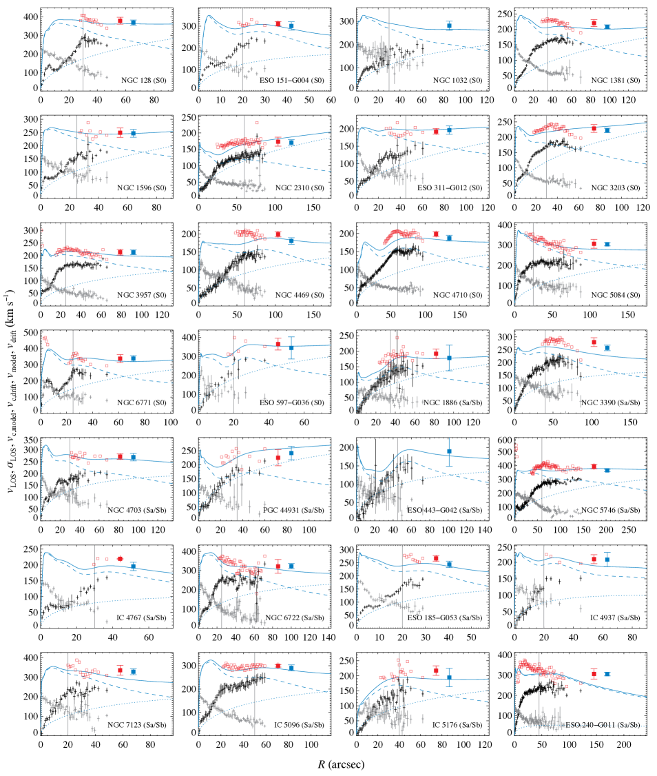
We calculate the asymmetric drift-corrected stellar velocity, $v_{\mathrm{drift}}$, using the observed stellar kinematics presented in Chung & Bureau (2004). In order to more accurately measure the local circular velocity we attempt to correct these observations for the effects of line-of-sight integration and asymmetric drift using the same recipe as used in BAM06, which we describe briefly below. We make no attempt to improve this recipe, since one of our goals is to assess the biases in previous determinations of the TFR based on stellar kinematics. The raw observations and their corrected values are shown in Fig. 1.

The line-of-sight correction for an edge-on disc assumes that the local azimuthal velocity $v_{\phi}(R)$ at a galactocentric distance $R$ (in the galaxy’s cylindrical coordinate system $(R,\phi,z)$) is related to $v_{\mathrm{LOS}}(x^{\prime})$, the luminosity-weighted mean line-of-sight velocity at a projected distance from the galaxy centre $x^{\prime}$, by the equation

$$v_{\mathrm{LOS}}(x^{\prime})=\frac{\int_{0}^{\infty}v_{\phi}(R)\rho(R)\cos\phi\,\mathrm{d}z^{\prime}}{\int_{0}^{\infty}\rho(R)\,\mathrm{d}z^{\prime}}.$$ (1)

Following the notation of, e.g., Binney & Tremaine (2008), $(x^{\prime},y^{\prime},z^{\prime})$ is the observer’s coordinate system on the sky, in which the $x^{\prime}$ axis is aligned with the projected major axis of the galaxy and the $z^{\prime}$ axis is along the line of sight. $\rho(R)$ is the luminosity density. The integral is evaluated along that line-of-sight $z^{\prime}$. By assuming that the local streaming velocity $v_{\phi}$ is independent of $R$, one can use the above relationship to infer it. This assumption is valid only if $R$ is at least the radius at which the intrinsic circular velocity curve flattens. To evaluate these integrals we assume $\rho(R)$ is an exponential disc of scale length $R_{\mathrm{d}}$, which we measure from the major-axis surface brightness profiles of our $K_{S}$-band images at radii outside the bulge (Bureau et al., 2006).

We then apply a correction for asymmetric drift to $v_{\phi}(R)$ to derive $v_{\mathrm{c,drift}}(R)$, an estimate of the true local circular velocity:

$$v_{\mathrm{c,drift}}^{2}(R)=v_{\phi}^{2}(R)+\sigma_{\phi}^{2}(R)\left(2\frac{R}{R_{\mathrm{d}}}-1\right),$$ (2)

where $\sigma_{\phi}(R)$ is the azimuthal stellar velocity dispersion. This equation is derived from the Jeans equations (Jeans 1922; Binney & Tremaine 2008) by assuming a thin disc in a steady state and the epicyclic approximation ($\sigma_{\phi}^{2}/\sigma_{R}^{2}=0.5$ for constant $v_{\phi}$). To estimate $\sigma_{\phi}(R)$, we assume that it is equal to an exponential fit to the observed stellar line-of-sight velocity dispersion $\sigma_{\mathrm{LOS}}(x^{\prime})$. This assumption is of course flawed, since the observed dispersion includes a contribution from the changing component of the azimuthal velocity along the line-of-sight. This effect will bias the asymmetric drift correction to be too high. However, the error is small in practice, and, crucially for the present work, it is not a strong function of galaxy type in the range S0–Sb. Under the assumptions described above, for disks with typical levels of pressure support ($v_{\phi}/\sigma_{\phi}\sim 5$ at the relevant radii $\approx 2$ – $4\,R_{\mathrm{d}}$), numerical integration shows that the error introduced by wrongly assuming $\sigma_{\phi}(R)=\sigma_{\mathrm{LOS}}(x^{\prime})$ causes $v_{\mathrm{c,drift}}$ to overestimate the true circular velocity by $\approx 0.04\pm 0.01$ dex. This error is almost independent of $v_{\phi}/\sigma_{\phi}$ in the range $2\leq v_{\phi}/\sigma_{\phi}\leq 20$, a quantity which is in any case independent of morphological type for our sample.

Finally, the local circular velocity of the mass model, $v_{\mathrm{c,model}}$, is derived from the dynamical models presented in WBC09. In that work, we modelled the mass distribution of each galaxy by assuming it is composed of an axisymmetric stellar component with a constant mass-to-light ratio and a spherical NFW dark halo (Navarro et al., 1997). The axisymmetric stellar component is based on an analytic fit to the observed near-infrared photometry of the composite bulge and disk. The absence of a triaxial bar component in our models does not significantly affect either the global properties of the models or the local kinematics at the large radii relevant to the TFR (see section 5.5.3 of WBC09 for a more extensive discussion of this issue). We assumed a particular relationship between halo mass and concentration (Macciò et al., 2008). We determined the three parameters of the models (the stellar mass-to-light ratio, virial halo mass and orbital anisotropy) by comparing the observed stellar second velocity moment $v_{\mathrm{rms}}(x^{\prime})=[v_{\mathrm{LOS}}^{2}(x^{\prime})+\sigma_{\mathrm{LOS}}^{2}(x^{\prime})]^{1/2}$ along the major axis to that predicted by solving the Jeans equations assuming a constant anisotropy (parametrized as $\beta_{z}=1-\sigma_{z}^{2}/\sigma_{R}^{2}$). The solution of the Jeans equations under these assumptions is described in Cappellari (2008). Note that while $v_{\mathrm{c,drift}}$ described above is weakly affected by our assumptions that $\sigma_{\phi}^{2}/\sigma_{R}^{2}=0.5$ and $\sigma_{\phi}(R)=\sigma_{\mathrm{LOS}}(x^{\prime})$, $v_{\mathrm{c,model}}$ suffers from no such biases. Our solutions of the Jeans equation are constrained by a fit to the observed second velocity moment along the line-of-sight. The second moment is strictly independent of $\sigma_{\phi}^{2}/\sigma_{R}^{2}$ so no assumption for this ratio is required, and the implementation rigorously accounts for line-of-sight integration.

To construct a TFR, the radial profiles of the asymmetric-drift corrected stellar kinematics, $v_{\mathrm{c,drift}}$ and of the model circular velocity, $v_{\mathrm{c,model}}$ must be characterized by a single number, $v_{\mathrm{drift}}$ and $v_{\mathrm{model}}$ respectively. We do this by determining the flat region of the observed rotation curve by eye. We then take $v_{\mathrm{drift}}$ to be the mean of the values of $v_{\mathrm{c,drift}}$ beyond this point. The continuous Jeans modelled circular velocity curve is evaluated at the same radii as the observed stellar kinematics. Its mean in the flat region of the observed rotation curve gives $v_{\mathrm{model}}$Ȯf course, it is possible to evaluate the circular velocity of the models at arbitrary radii, but by restricting ourselves to those radii for which we have stellar kinematic observations, we avoid using the mass models in regions where they are not constrained by the data. Fig. 1 shows these calculations for all sample galaxies.

2.3 Comparison

Figure 2: Comparisons of the circular velocities of the mass models ($v_{\mathrm{model}}$), observed stellar kinematics corrected for asymmetric drift ($v_{\mathrm{drift}}$) and rotational velocities derived from global H i line widths ($v_{\mathrm{H\,\textsc{i}}}$) and ionized gas position-velocity diagrams ($v_{\mathrm{gas}}$). The solid blue triangles are the Sa–Sb galaxies from our sample and the solid red circles the S0s. The open red circles are the S0s presented in BAM06. They do not estimate $v_{\mathrm{model}}$ so, in order to place these galaxies on the plot, we assume $v_{\mathrm{drift}}\approx v_{\mathrm{model}}$ for them.

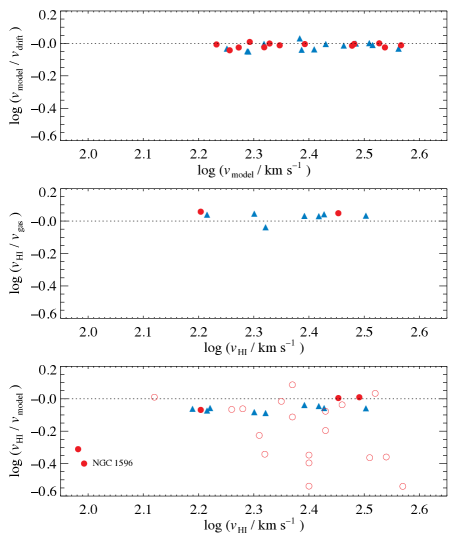
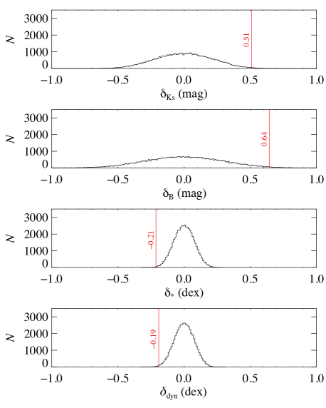
A comparison of the four measures of rotation is shown in Fig. 2. The upper panel demonstrates that $\left<\log(v_{\mathrm{model}}/v_{\mathrm{drift}})\right>$ $=-0.015\pm 0.003$ dex with an rms scatter of 0.019 dex for both spirals and S0s. This small difference, which is on average less than 4 per cent, is probably due to the additional approximations and assumptions introduced in the asymmetric drift correction compared to the Jeans models. We note in particular that it is consistent with the error due to assuming $\sigma_{\phi}(x^{\prime})=\sigma_{\mathrm{LOS}}(x^{\prime})$, as discussed in Section 2.2. The absolute offset between these measures is not significant in the context of the TFR and, crucially, there is no evidence of any systematic difference between S0s and spirals. The scatter is also extremely small. Since both $v_{\mathrm{drift}}$ and $v_{\mathrm{model}}$ are derived from the observed stellar kinematics, their close agreement is not of itself independent proof of the accuracy with which they trace the true circular velocity. The agreement of $v_{\mathrm{drift}}$ with the results of detailed and robust Jeans modelling does suggest, however, that the approximations inherent in eqns. (1–2) yield an approximately valid solution of the Jeans equations.

The middle panel demonstrates fairly good agreement between the two measures based on gas, $v_{\mathrm{H\,\textsc{i}}}$ and $v_{\mathrm{gas}}$. $\left<\log(v_{\mathrm{H\,\textsc{i}}}/v_{\mathrm{gas}})\right>=0.032\pm 0.009$ dex with a rms scatter of 0.029 dex. There is some evidence that $v_{\mathrm{H\,\textsc{i}}}$ systematically exceeds $v_{\mathrm{gas}}$ by 5 – 10 per cent. Statistics are poorer because gas is rare in S0s by definition, but there is no evidence of any systematic difference between $v_{\mathrm{H\,\textsc{i}}}/v_{\mathrm{gas}}$ in S0s and spirals.

However, the bottom panel of Fig. 2 shows that $v_{\mathrm{model}}$ (and therefore $v_{\mathrm{drift}}$) does not in general agree $v_{\mathrm{H\,\textsc{i}}}$ (and thus $v_{\mathrm{gas}}$): $\left<\log(v_{\mathrm{H\,\textsc{i}}}/v_{\mathrm{model}})\right>=-0.094\pm 0.031$ dex with a rms scatter of 0.115 dex (or $-0.18\pm 0.043$ dex with a rms scatter of 0.243 dex if the BAM06 galaxies are included). Some of this difference and scatter is caused by pathological cases of $v_{\mathrm{H\,\textsc{i}}}$ derived from single dish measurements, i.e. spatially unresolved measurements of 21 cm signal from galaxies with a warped gas disc, polar rings or gas-rich nearby companions that fall within the telescope beam (e.g. this is almost certainly the case for the S0 galaxy NGC 1596, see Chung et al. 2006).

But even when possible pathological cases are avoided, for example by ignoring S0 galaxies, which are more likely to be problematic, there remains a clear systematic offset: $\left<\log(v_{\mathrm{H\,\textsc{i}}}/v_{\mathrm{model}})\right>=-0.063\pm 0.005$ dex (15 per cent) with 0.02 dex rms scatter for the spirals in our sample. For these galaxies, the rotational velocity derived from the global H i line width is significantly and systematically smaller than that derived from stellar kinematics or dynamical modelling. Because $v_{\mathrm{H\,\textsc{i}}}$ is derived from spatially unresolved data, this could be explained by the global H i line width probing the local gas velocity out to different radii than our typical stellar kinematic data (Noordermeer et al., 2007).

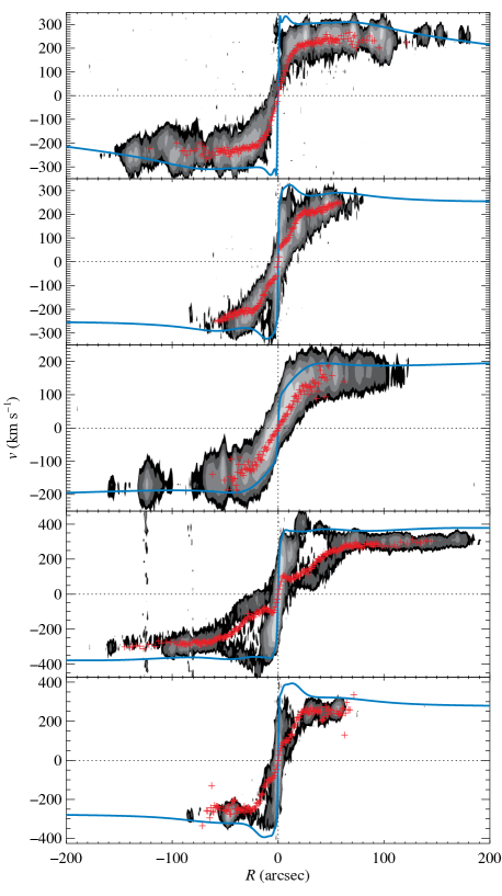
We find a similar systematic difference between $v_{\mathrm{model}}$ (or $v_{\mathrm{drift}}$) and $v_{\mathrm{gas}}$: $\left<\log(v_{\mathrm{gas}}/v_{\mathrm{model}})\right>=-0.086\pm 0.008$. $v_{\mathrm{gas}}$ is derived from a spatially resolved PVD taken from the same long-slit optical spectrum with which we derive the stellar kinematics. We can therefore verify directly that it does not suffer from either pathological problems related to gas-rich companions, warps or polar rings, or doubt about the radii probed compared to our stellar kinematics. We show this in Fig. 3 for the five sample galaxies with optical emission that extends to the disk. It is clear that the stars and gas are associated with the same galaxy and are observed at similar radii. Therefore, unless light-emitting gas is absent from the tangent point along the line-of-sight in these edge-on galaxies (a possibility we cannot rule out), the emission line gas kinematics and absorption line stellar kinematics should imply the same local circular velocity and the same single characteristic measure of rotation, ($v_{\mathrm{gas}}$, $v_{\mathrm{drift}}$ or $v_{\mathrm{model}}$).

But in these five galaxies galaxies, the stars and gas rotate with essentially the same velocity as a function of position in the outer, flat parts of the observed rotation curve. The stars have non-negligible dispersion so we know they do not trace the local circular velocity by an amount that can be calculated using the Jeans equations. Given this observation, it is not surprising that $v_{\mathrm{gas}}$ is significantly less than $v_{\mathrm{model}}$.

In summary, while agreement between $v_{\mathrm{gas}}$ and $v_{\mathrm{H\,\textsc{i}}}$ is fairly good, and from this we conclude that $v_{\mathrm{model}}$ and $v_{\mathrm{drift}}$ (based on stars seen in absorption) do not imply the same circular velocity as $v_{\mathrm{H\,\textsc{i}}}$ and $v_{\mathrm{gas}}$ (based on gas seen in emission). This is not a new result. In early-type disc galaxies, the observed stellar kinematics and the well-understood Jeans equations often imply a local circular velocity greater than the observed rotational velocity of gas (e.g. Kent, 1988; Kormendy & Westpfahl, 1989; Bertola et al., 1995; Cinzano et al., 1999; Corsini et al., 1999; Cretton et al., 2000; Vega Beltrán et al., 2001; Pizzella et al., 2004; Krajnović et al., 2005; Weijmans et al., 2008; Young et al., 2008). This puzzle is made more acute by the small velocity dispersions observed in the emission line PVDs. We will return to the gas dispersion in a future work.

Figure 3: Comparisons of [N ii] $\lambda 6584$ position–velocity diagrams, stellar kinematics, and the circular velocity implied by Jeans modelling for the five galaxies in the sample with optical emission that extends to the disc. From top to bottom: ESO 240-G11, IC 5096, IC 5176, NGC 5746 and NGC 6722. The filled contours are the continuum-subtracted optical spectra originally presented in Bureau & Freeman (1999). The observed mean stellar velocities (Chung & Bureau, 2004) and the circular velocity profiles inferred from detailed Jeans modelling of the light distribution and stellar kinematics (WBC09) are overplotted as red crosses and blue lines respectively.

A definitive resolution of this issue is outside the scope of the present work and, fortunately, it is unnecessary for our goals. For the purposes of comparing TFRs (or for determining relative distances; see e.g. Courtois et al. 2009), it does not matter which measure is ‘right’, as long as we use the same measure for the two samples and the measure chosen does not introduce a systematic bias between samples. We see no evidence of this in our data, for any of the four measures explored.

Our conclusions in this section have three consequences for previous works that measure the TFR of S0 galaxies using stellar kinematics corrected for asymmetric drift (e.g. Neistein et al., 1999; Hinz et al., 2001, 2003, BAM06): (i) the asymmetric drift correction they use yields similar results to detailed Jeans modelling; (ii) the drift correction does not seem to introduce a systematic bias between spirals and S0s and, if applied to samples of both spirals and S0s, can indeed be used to compare the TFRs of the two classes; (iii) however, a TFR derived from asymmetric drift-corrected stellar kinematics cannot be directly compared to TFRs derived from global H i line widths or resolved emission line PVDs, as these previous authors did. As we argue above, such comparisons are not a priori justified and, in the case of both our sample and the larger sample of BAM06, they appear to introduce systematic errors that, on a Tully-Fisher plot, are of the same order (and in the same direction) as the TFR offsets that are usually interpreted as luminosity evolution. The conclusions of previous works regarding the offset of the S0 TFR should therefore be treated with caution. In addition, given the large scatter we observe in $\log(v_{\mathrm{H\,\textsc{i}}}/v_{\mathrm{model}})$ and $\log(v_{\mathrm{H\,\textsc{i}}}/v_{\mathrm{drift}})$, it is far from clear that any simple additive or multiplicative correction could eliminate the bias.

For our sample, we are able to side-step this issue completely by using a single measure of rotation for both spirals and S0s. In this way we compare the TFRs of S0, Sa and Sb galaxies in a manner which is not subject to the possible systematics discussed above. We adopt $v_{\mathrm{model}}$ as our fiducial measure of rotation for both spirals and S0s. The figures and discussion that follow use only this measure.

3 Sample and data

Table 1: Sample.

Galaxy	$M_{K_{S}}$	$M_{B}$	$\log(M_{\star}/M_{\odot})$	$\log(M_{\mathrm{dyn}}/M_{\odot})$	$R_{\mathrm{d}}$	$v_{\mathrm{model}}$	$v_{\mathrm{drift}}$	$v_{\mathrm{H\,\textsc{i}}}$	$v_{\mathrm{gas}}$	2MRS LDC	Cluster
	(mag)	(mag)			(arcsec)	(km s-1)	(km s-1)	(km s-1)	(km s-1)	group size
(1)	(2)	(3)	(4)	(5)	(6)	(7)	(8)	(9)	(10)	(11)	(12)
S0
NGC 128	$-25.35$	$-21.40$	11.47	11.56	16.7	369	379	…	…	…
ESO 151-G004	$-24.85$	$-20.41$	11.40	11.46	8.2	301	311	…	…	a
NGC 1032	$-24.47$	$-20.71$	11.13	11.22	33.0	281	…	284	254	…
NGC 1381	$-22.76$	$-18.77$	10.49	10.59	12.3	208	220	…	…	43	Fornax
NGC 1596	$-22.86$	$-18.98$	10.56	10.66	20.5	247	249	98	…	30
NGC 2310	$-22.48$	$-19.43$	10.25	10.48	25.2	171	173	…	…	…
ESO 311-G012	$-23.06$	$-19.92$	10.45	10.53	28.3	196	192	96	…	…
NGC 3203	$-23.89$	$-19.99$	10.76	10.94	16.3	222	228	…	…	210	Hydra
NGC 3957	$-23.29$	$-19.20$	10.76	10.85	19.1	213	213	…	178	13
NGC 4469	$-23.01$	$-19.02$	10.56	10.68	16.5	180	199	…	…	300	Virgo
NGC 4710	$-23.47$	$-19.40$	10.56	10.68	23.6	187	199	160	140	300	Virgo
NGC 5084	$-24.73$	$-21.85$	11.16	11.22	34.7	303	306	310	…	15
NGC 6771	$-25.08$	$-20.81$	11.40	11.46	16.2	337	337	…	284	97
ESO 597-G036	$-25.36$	$-20.70$	11.58	11.73	14.4	345	365	…	…	3
Sa–Sb
NGC 1886	$-22.90$	$-19.73$	10.47	10.63	14.5	178	192	155	…	…
NGC 3390	$-24.90$	$-21.49$	11.19	11.27	20.4	257	279	210	229	210	Hydra
NGC 4703	$-25.43$	$-20.92$	11.38	11.49	29.2	269	272	246	229	80
PGC 44931	$-24.46$	$-21.33$	11.07	11.27	21.1	242	225	200	180	80
ESO 443-G042	$-23.49$	$-20.21$	10.76	10.90	11.4	190	…	166	…	38
NGC 5746	$-25.64$	$-22.30$	11.63	11.75	69.1	365	393	319	295	45
IC 4767	$-23.69$	$-19.72$	10.93	10.97	8.2	195	219	…	…	97
NGC 6722	$-25.38$	$-21.97$	11.49	11.60	12.5	323	322	…	263	97
ESO 185-G053	$-24.22$	$-20.09$	11.01	11.06	5.0	244	267	…	…	42
IC 4937	$-24.67$	$-20.46$	11.18	11.24	18.7	208	210	…	…	3
NGC 7123	$-25.29$	$-20.81$	11.35	11.40	19.2	327	335	…	…	…
IC 5096	$-24.93$	$-21.21$	11.27	11.36	14.5	290	300	262	244	5
IC 5176	$-23.31$	$-19.95$	10.60	10.72	20.9	194	217	164	150	…
ESO 240-G011	$-24.79$	$-21.56$	11.56	11.57	35.7	305	306	268	243	3

Notes. Sample divided into S0s and spirals based on classifications of Jarvis (1986), de Souza & Dos Anjos (1987), Shaw (1987) and Karachentsev et al. (1993). (1) Galaxy name. (2)–(3) Total $K_{S}$-band and $B$-band absolute magnitude. (4)–(5) Total stellar and dynamical mass. (6) Disk scale length measured using $K_{S}$-band images presented in Bureau et al. (2006). (7) Circular velocity derived from the best-fit mass model presented in WBC09. (8) Rotational velocity derived from the observed stellar kinematics presented in Chung & Bureau (2004), corrected for line-of-sight effects and asymmetric drift. Missing values are cases where the drift correction was too large to be considered reliable. (9) Rotational velocity derived from the global H i line width, i.e. the quantity vrot from HYPERLEDA where available. (10) Ionized gas rotational velocity measured by a Gaussian fit to [N ii] position-velocity diagrams presented in Bureau & Freeman (1999). (11) Number of companion group members in the Low Density Contrast 2MRS Group Catalog (Crook et al., 2007). Ellipses indicate that a galaxy was not found in the catalog, implying that it had 2 or fewer nearby companions. (^a) ESO 151-G004 is not present in the 2MASS Extended Source Catalog (Jarrett et al., 2000) and so is not included in the 2MRS database. (12) Cluster membership. For full details of how the quantities in Columns (2)–(10) were determined, see Section 2.2 and Section 3.

To make the reliable comparison we described in the previous section, we use the sample of 14 early-type spirals (Sa and Sb) and 14 S0s presented in Table 1. Dynamical models of these galaxies were constructed in WBC09. All of the galaxies are oriented close to edge-on (within $\approx 5^{\circ}$). Many of the galaxies have boxy bulges, which are believed to be bars viewed side-on (e.g. Kuijken & Merrifield, 1995; Merrifield & Kuijken, 1999; Bureau & Freeman, 1999; Chung & Bureau, 2004), and it was to probe these bulges that the sample was constructed and observed. The bars should not, however, affect the results we present here because we use measures of rotational velocity well outside the boxy bulge region. The fraction of galaxies with boxy bulges in the sample ($\approx 75$ per cent) is not in any case significantly different to the fraction of barred galaxies in the local universe ($\approx$ 65 per cent; see, e.g. Eskridge et al., 2000; Whyte et al., 2002; Marinova & Jogee, 2007).

The sample was selected without regard for environment, and so includes galaxies in a wide range of environments. Two S0s are members of the Virgo cluster, an S0 and a spiral are members of the Hydra cluster, and an S0 is a member of the Fornax cluster. Cross-referencing our sample with the 2MASS Redshift Survey (2MRS) Group Catalog (Crook et al., 2007) demonstrates that the remainder of the sample is made up of members of intermediate-size groups and relatively isolated galaxies.

All the galaxies are relatively bright and fast-rotating, and the spirals and S0s cover the same range of luminosities. This means that we are not vulnerable to variation in the slope of the TFR at the low or high mass end, as has been observed (e.g. Peletier & Willner, 1993; Noordermeer & Verheijen, 2007). We further note that the sample contains some very bright S0s, such as ESO 151-G004 and NGC 6771, that have large boxy bulges. If these bulges are in fact bars, and therefore the products of secular evolution, then these particular bright S0s are unlikely to be the elliptical-like products of major mergers, as has previously been suggested (Poggianti et al., 2001; Mehlert et al., 2003; Bedregal et al., 2008; Barway et al., 2009).

Figure 4: Tully-Fisher relations for our samples of S0 and spiral galaxies. From top to bottom, as a function of $v_{\mathrm{model}}$: total absolute $K_{S}$-band luminosity, total absolute $B$-band luminosity, total stellar mass and total dynamical mass. Spiral galaxies are shown as blue triangles and S0 galaxies as red circles. A median error bar is shown in the top left corner of each plot. The best fit relations found by inverse regression are shown as solid lines (blue for spirals, red for S0s). Their parameters are given in Table 2. The dashed, dotted and dot-dashed lines are a selection of TFRs found by previous authors for different morphological types. See text for a full discussion of these relations.

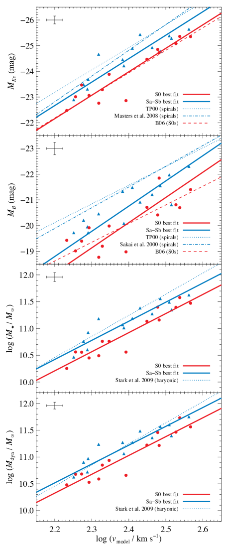
In Fig. 4 we present the spiral and S0 TFRs as functions of $K_{S}$-band luminosity, $B$-band luminosity, stellar mass and dynamical mass, all discussed below. Throughout this work we assume an absolute solar magnitude $M_{Ks,\odot}=3.29$ mag (Blanton & Roweis, 2007).

Firstly, all the vertical axes in Fig. 4 require a distance estimate for each galaxy. As described in WBC09, we use surface brightness fluctuation (SBF) estimates where available (NGC 1381 from Jensen et al. 2003 and NGC 1596 from Tonry et al. 2001) and the Virgo cluster distance where appropriate (NGC 4469 and NGC 4710, Mei et al. 2007). For all other galaxies we adopt the redshift distance presented in the NASA/IPAC Extragalactic Database, corrected for a Virgocentric flow model (Mould et al., 2000). We assume a Wilkinson Microwave Anisotropy Probe five-year (WMAP5) cosmology ($H_{0}=70$ km s^-1 Mpc^-1, Komatsu et al. 2009). Of course, we avoid distance estimates derived from TFRs.

The total apparent magnitude at $K_{S}$-band is measured using the analytically derived total light in the multi-Gaussian expansions (Emsellem et al., 1994; Cappellari, 2002) of our near-infrared images, as described and tabulated in WBC09. The total apparent magnitude at $B$-band is taken from HYPERLEDA (Paturel et al., 2003). We apply corrections for Galactic ($A_{\mathrm{G}}$) and internal ($A_{\mathrm{i}}$) extinction in both bands using the Galactic dust maps of Schlegel et al. (1998) and the internal extinction correction presented in Bottinelli et al. (1995), as tabulated in HYPERLEDA (Paturel et al., 2003), both of which we transform to the appropriate bands using the extinction law of Cardelli et al. (1989), implying that $A_{\mathrm{G}}(K_{S})/A_{G}(B)=A_{\mathrm{i}}(K_{S})/A_{\mathrm{i}}(B)=0.084$. The internal extinction correction is a function of both bulge-to-disc ratio and morphological type. This correction is $\lesssim 0.1$ mag at $K_{S}$-band for our spirals and smaller still for the S0s.

With the exception of the Virgo galaxies and the two galaxies with SBF distances, we adopt characteristic distance errors corresponding to a 200 km s^-1 uncertainty in the flow model (e.g. Tonry et al., 2000), and 0.05 mag uncertainties in the apparent magnitudes. These uncertainties completely overwhelm any error in the Galactic or internal extinction at $K_{S}$-band. At $B$-band, we adopt uncertainties of 0.16 mag in Galactic extinction (Schlegel et al., 1998) and 0.1 mag in the internal extinction. We emphasize, however, that internal extinction corrections in edge-on spiral galaxies are both large and uncertain. The $B$-band TFR is problematic with even favourably inclined spirals, but with our edge-on sample the internal extinction correction and its uncertainties may introduce significant systematic errors. The $B$-band data are therefore included in this work merely to aid comparison with previous work, and we do not make use of these results in our interpretation.

The stellar mass, $M_{\star}$, is derived from the total absolute $K_{S}$-band luminosity and the constant stellar mass-to-light ratio, $(M/L)_{K_{S}}$, of each galaxy determined in WBC09. As described in Section 2.2, this uses dynamical methods that make assumptions about the dark halo and stellar dynamics, but are not vulnerable to zero-point or colour-dependent uncertainties due to the initial mass function or stellar evolution.

The dynamical mass, $M_{\mathrm{dyn}}$, is estimated using the total absolute $K_{S}$-band luminosity and the dynamical mass-to-light ratio at $K_{S}$-band for each galaxy, also determined in WBC09 in which it is referred to as $(M/L)_{K_{S},\mathrm{nohalo}}$. Unless there is no dark matter (or its distribution closely follows that of the luminous matter), the dynamical $(M/L)$ ratio is likely to be a quantity that varies significantly within a galaxy, increasing toward the edge of the optical disc where dark matter normally begins to dominate. The value we use is, however, effectively an average for each galaxy within the radii constrained by the stellar kinematic data, typically 2-3 $R_{\mathrm{e}}$(where $R_{\mathrm{e}}$is the projected $K_{S}$-band half-light radius), but dominated by the central regions. Because of this, $M_{\mathrm{dyn}}$ is a somewhat ill-defined quantity.

An alternative approach would be to adopt the mass within the three-dimensional half-light volume, $M_{1/2}$. We show how this can be evaluated from observations or models of the circular velocity in disc galaxies in Appendix A. We also show there that, in practice, $2M_{1/2}=M_{\mathrm{dyn}}$ to within 13 per cent. Neither choice is optimal but in the context of the present work, we can think of no reason why one choice or the other would introduce systematic biases that vary between spirals and S0s. The choice is therefore somewhat arbitrary and has no affect on the discussion of the relationship between spirals and S0s that follows where we use $M_{\mathrm{dyn}}$. This follows precedent (it is the definition used by, e.g., Magorrian et al. 1998, Häring & Rix 2004 and Cappellari et al. 2006) and avoids the possible concern that the argument we present in Section 5.2 is circular, but we emphasize that $M_{1/2}$ gives the same results and is a better defined quantity.

For reference, we show in Fig. 4 the spiral TFRs determined using global H i line widths at $K$-band by TP00, at $K_{S}$-band by Masters et al. (2008) and at $B$-band by TP00 and Sakai et al. (2000). We do this assuming that the global H i line width, once corrected for inclination, broadening and turbulent motion, is exactly twice the rotational velocity. The zero points of the TP00 and Sakai et al. (2000) TFRs were determined using known Cepheid distances to 4 galaxies in the case of TP00 at $K$-band (1 Sab, 2 Sb and 1 Sc; see the companion paper by Rothberg et al. 2000), 24 galaxies for TP00 at $B$-band (3 Sab, 14 Sb – Sc and 7 Scd – Sd) and 21 galaxies for Sakai et al. (2000) (3 Sa – Sab, 16 Sb – Sc and 2 Scd). We position the Masters et al. (2008) $K_{S}$-band TFR on our plots using our adopted value of $H_{0}$. The difference between the two $K$-band and two $B$-band relations gives an idea of the uncertainty in the absolute location of the late-type spiral TFR (the difference between the $K$-band filter used by TP00 and the 2MASS $K_{S}$-band filter is not significant in this context). These comparison spiral TFRs are unconstrained by observations above $\log(v/\mathrm{km\ s^{-1}})\approx 2.45$, while a third of our sample is above this value.

Unlike BAM06, we do not shift the zero-points of the TP00 TFRs by $-0.207$ mag. BAM06 did this to make the value of $H_{0}$ implied by TP00’s data ($77\pm 8$ km s^-1 Mpc^-1) consistent with their adopted value ($70$ km s^-1 Mpc^-1). However, we believe that this correction was in error, since the absolute locations of the TP00 TFRs were set by independent Cepheid distances, which imply rather than assume a particular value of $H_{0}$.

We also show an extrapolation to high mass systems of the baryonic TFR presented in Stark et al. (2009), which was calibrated using gas-dominated dwarf galaxies (hence minimizing uncertainties associated with the stellar mass-to-light ratio). Neither of our mass estimates $M_{\star}$ or $M_{\mathrm{dyn}}$ are designed to reproduce the baryonic mass $M_{\mathrm{bar}}$ used by Stark et al. (2009). In practice, however, one expects $M_{\star}\approx M_{\mathrm{bar}}$ to within a few per cent for gas-poor S0s and to within perhaps ten per cent for giant Sa–Sb spirals, while $M_{\mathrm{dyn}}\approx M_{\mathrm{bar}}$ to within a factor of 2 for both S0s and spirals (dark matter is no more than 50 per cent of the mass within the optical radius of disk galaxies, e.g. van Albada & Sancisi 1986; Persic et al. 1996; Palunas & Williams 2000; Cappellari et al. 2006; Kassin et al. 2006, WBC09). The comparison of our stellar and dynamical mass TFRs to the baryonic TFR is therefore meaningful, and we note that the Stark et al. (2009) TFR is broadly consistent with our spirals. The good agreement gives us confidence in our mass models.

It is crucial to emphasize that at no point in our analysis do we do anything that might systematically affect the S0s in the sample differently to the spirals. One slight but unavoidable observational bias may be introduced by the presence of dust along the major axes. If the slit is placed exactly on the major axis, then absorption by dust may make it impossible to recover the full line-of-sight velocity distributions (LOSVDs). Depending on the optical thickness, this may truncate the low velocity wing or, in very dusty discs, the high velocity peak of the LOSVDs. When Gaussians are fitted to these distribution (Chung & Bureau, 2004), this could therefore increase or, perhaps more likely, decrease the derived line-of-sight velocities. This effect would propagate into the rotation curves from which $v_{\mathrm{model}}$ and $v_{\mathrm{drift}}$ are derived, and also into the mass-to-light ratios inferred in WBC09, from which $M_{\star}$ and $M_{\mathrm{dyn}}$ are derived. However, in cases where the dust absorption was strong, the slit was simply shifted from the major axis by $\approx 2$ arcsec to ensure the full LOSVD was sampled, and the objects with strong dust lanes were selected to be very slightly away from perfectly edge-on (Bureau & Freeman, 1999).

If the rotational velocity is a strong function of $z$, the height above the equatorial plane in the cylindrical coordinate system of the galaxy $(R,\phi,z)$, this intentional shift could itself bias the velocities and inferred masses in dustier galaxies (i.e. spirals). In a future work (Williams et al., in preparation), we will present pseudo-integral-field data (i.e. a sparse velocity fields constructed from multiple long-slit positions) for six of the galaxies in the present sample. In these data we see no evidence that $\mathrm{d}\,v/\mathrm{d}\,|z|\neq 0$ in the disks of five of the galaxies. At most, there is a gradient of $-30$ km s^-1 kpc^-1 in the disk of NGC 7123. This is broadly consistent with observations of planetary nebulae in the edge-on spiral NGC 891 (Merrifield et al., 2010) and of extraplanar gas (e.g. NGC 891, Heald et al. 2007, Oosterloo et al. 2007; NGC 4302 and NGC 5775, Heald et al. 2007; the Milky Way, Levine et al. 2008), which find a typical falloff in rotation $\mathrm{d}v/\mathrm{d}|z|\approx-20$ km s^-1 kpc^-1 In the worst case scenario, in which all our spirals (and none of the S0s) suffered from absorption strong enough to require shifting the slit, the spiral velocities would typically be biased by $\lesssim-0.02$ dex. We estimate that the overall effect on our sample of spirals, most of which did not require this slit shift, may be to bias their velocities by up to $\approx-0.01$ dex. In practice, the slit was 1.8 arcsec wide and rather difficult to align precisely for both spirals and S0s. This imprecision, which introduces velocity scatter in both samples, likely overwhelms any systematic velocity falloff in the spirals due to intentionally shifting the slit.

4 Fitting procedure

For each measure of luminosity or mass as a function of $x=\log(v_{\mathrm{model}}/\mathrm{km\ s^{-1}})$, we simultaneously fit a straight line of the form $y=a(x-2.4)+b$ to the spiral galaxies and $y=a(x-2.4)+b+\delta$ to the S0s. The two straight lines are therefore constrained to have the same slope, $a$, but they have zero-points which differ by $\delta$. In separate fits to the two samples, we find that their slopes are consistent within the uncertainties. Constraining them to be equal therefore significantly simplifies the interpretation of our results in terms of zero-point evolution. The $x=2.4$ reference value is defined to minimize the covariance between errors in $a$ and $b$ (e.g. Tremaine et al., 2002). Its choice does not affect the results of this work, in which were are mainly interested in the zero point offset $\delta$.

To find the optimal combination of $a$, $b$ and $\delta$ for a given scatter, we define and minimize the figure of merit

$$\begin{split}\chi^{2}&\equiv\sum^{N_{\mathrm{Sa\,Sb}}}_{i=0}\frac{1}{\sigma_{i}^{2}}\{y_{i}-[a(x_{i}-2.4)+b]\}^{2}\\ &\quad+\sum^{N_{\mathrm{S0}}}_{i=0}\frac{1}{\sigma_{i}^{2}}\{y_{i}-[a(x_{i}-2.4)+b+\delta]\}^{2},\end{split}$$ (3)

where $N_{\mathrm{Sa\,Sb}}$ is the number of spirals, $N_{\mathrm{S0}}$ the number of S0s and

$$\sigma_{i}^{2}\equiv\sigma_{y,i}^{2}+a^{2}\sigma_{x,i}^{2}+\sigma_{\mathrm{int}}^{2}.$$ (4)

The extra scatter $\sigma_{\mathrm{int}}$ is iteratively adjusted to ensure that

$$\chi_{\mathrm{red}}^{2}\equiv\frac{\chi^{2}}{(N_{\rm Sa,Sb}+N_{\rm S0}-3)}\approx 1.$$ (5)

If the observational errors for each galaxy $\sigma_{x,i}$ and $\sigma_{y,i}$ are well-estimated then $\sigma_{\mathrm{int}}$ is the intrinsic, astrophysical scatter in the TFR.

We also define a total rms scatter $\sigma_{\mathrm{tot}}$, essentially a weighted mean of the scatter of the data about the fits (and therefore in the same units as the $y$-axis):

$$\begin{split}\sigma_{\rm tot}^{2}&\equiv\Bigg{(}\sum^{N_{\mathrm{Sa\,Sb}}}_{i=0}\frac{1}{\sigma_{i}^{2}}\{y_{i}-[a(x_{i}-2.4)+b]\}^{2}\\ &\quad+\sum^{N_{\mathrm{S0}}}_{i=0}\frac{1}{\sigma_{i}^{2}}\{y_{i}-[a(x_{i}-2.4)+b+\delta]\}^{2}\Bigg{)}\Bigg{/}\sum^{N_{\mathrm{gal}}}_{i=0}\frac{1}{\sigma_{i}^{2}}\end{split}$$ (6)

$$=\frac{\chi^{2}}{\sum_{i=0}^{N_{\mathrm{gal}}}1/\sigma_{i}^{2}},$$ (7)

where $N_{\mathrm{gal}}$ is the total number of both spiral and S0 galaxies. Comparing $\sigma_{\mathrm{tot}}$ with $\sigma_{\rm int}$ gives an idea of what fraction of the scatter is intrinsic and what fraction is due to measurement errors. We minimize equation (3) using the mpfit package (Markwardt, 2008).

Following previous analyses of the Tully-Fisher relation, we also fit the ‘inverse’ relation, i.e. we regress the observed rotational velocities rather than the luminosities or masses onto the model (see, e.g., TP00, Verheijen 2001, Pizagno et al. 2007 and references therein). We rewrite the spiral and S0 straight lines as $x=Ay+B+2.4$ and $x=Ay+B+2.4+\Delta$ and minimize

$$\begin{split}\chi^{2}_{\mathrm{inv}}&\equiv\sum^{N_{\mathrm{Sa\,Sb}}}_{i=0}\frac{1}{\varsigma_{i}^{2}}[x_{i}-(Ay_{i}+B+2.4)]^{2}\\ &\quad+\sum^{N_{\mathrm{S0}}}_{i=0}\frac{1}{\varsigma_{i}^{2}}[x_{i}-(Ay_{i}+B+\Delta+2.4)]^{2},\end{split}$$ (8)

where

$$\varsigma_{i}^{2}=\sigma_{x,i}^{2}+A^{2}\sigma_{y,i}^{2}+\varsigma_{\mathrm{int}}^{2}$$ (9)

and

$$\varsigma^{2}_{\mathrm{tot}}=\frac{\chi_{\mathrm{inv}}^{2}}{\sum_{i=0}^{N_{\mathrm{gal}}}1/\varsigma_{i}^{2}}.$$ (10)

To compare these values to those determined using the forward relation, we use the fact that a best-fitting inverse relation has an equivalent forward slope $1/A$, zero-point $-B/A$, offset $-\Delta/A$ and $y$-axis intrinsic and total scatters $A\varsigma_{\mathrm{int}}$ and $A\varsigma_{\mathrm{tot}}$. Our implementation of the fitting procedure described above is publicly available.

Forward and inverse fitting is only symmetric if there is no intrinsic scatter ($\sigma_{\mathrm{int}}=\varsigma_{\mathrm{int}}=0)$ (Tremaine et al., 2002). This is not generally the case and the slopes can be very different. In analyses of the TFR with observed data, it has been shown that there is a significant bias in the slope of the forward line of best fit (Willick, 1994), which is why the inverse relationship is usually preferred. The figures in this paper use this inverse fitting approach, but to aid comparison with future work, we present both forward and inverse fits in Table 2. The slopes of the forward and inverse fits to our data are indeed discrepant, often to the extent that they do not lie within each other’s error bars (especially at $B$-band). We are fortunate, however, that the choice of whether to use the forward or inverse relationship does not affect our conclusions, which depend entirely on the zero-point offset of the S0 TFR and the total scatter.

5 Discussion

5.1 The TFR zero-point offset at $K_{S}$-band and $B$-band

Table 2: Parameters of the best fitting TFRs, where $x=\log(v_{\mathrm{model}}/\mathrm{km\,s}^{-1})$, $y=a(x-2.4)+b$ for spirals and $y=a(x-2.4)+b+\delta$ for S0s.

$y$	$a$		$b$		$\delta$		$\sigma_{\rm int}$	$\sigma_{\rm tot}$
Forward regression
$M_{K_{S}}$	$-8.15$$\pm$	$0.76$	$-24.53$$\pm$	$0.11$	$0.55$$\pm$	$0.15$	0.27	0.37
$M_{B}$	$-7.67$$\pm$	$1.02$	$-20.82$$\pm$	$0.14$	$0.73$$\pm$	$0.20$	0.39	0.50
$\log(M_{\star}/M_{\odot})$	$3.45$$\pm$	$0.26$	$11.14$$\pm$	$0.04$	$-0.22$$\pm$	$0.05$	0.06	0.13
$\log(M_{\mathrm{dyn}}/M_{\odot})$	$3.34$$\pm$	$0.27$	$11.23$$\pm$	$0.04$	$-0.20$$\pm$	$0.05$	0.07	0.13
Inverse regression
$M_{K_{S}}$	$-9.13$$\pm$	$0.87$	$-24.49$$\pm$	$0.12$	$0.51$$\pm$	$0.16$	0.28	0.39
$M_{B}$	$-9.81$$\pm$	$1.26$	$-20.76$$\pm$	$0.16$	$0.64$$\pm$	$0.23$	0.44	0.56
$\log(M_{\star}/M_{\odot})$	$3.57$$\pm$	$0.27$	$11.13$$\pm$	$0.04$	$-0.21$$\pm$	$0.05$	0.06	0.13
$\log(M_{\mathrm{dyn}}/M_{\odot})$	$3.52$$\pm$	$0.28$	$11.22$$\pm$	$0.04$	$-0.19$$\pm$	$0.05$	0.08	0.13

Notes. $\sigma_{\mathrm{int}}$ is the intrinsic scatter required to yield $\chi_{\mathrm{red}}=1.00\pm 0.01$ and $\sigma_{\mathrm{tot}}$ is the total scatter (see equation 6). $a$ is in units of $y/x$, all other quantities are in units of $y$, i.e. magnitudes or dex of solar masses.

While the TFR zero point and offset are formally sensitive to the choice between forward or inverse regression, in practice they are almost unchanged by this choice. In the discussion that follows, we adopt the means of the forward and inverse values and their errors.

We detect a statistically significant difference between the zero-points of the TFRs of spiral and S0 galaxies (see Table 2). At a given $v_{\mathrm{model}}$, local S0s are $0.53\pm 0.15$ mag fainter at $K_{S}$-band and $0.68\pm 0.22$ mag fainter at $B$-band than local spirals. The systematic uncertainty is due to the slit positioning issue described at the end of Section 3. We emphasize again that the $B$-band offset we measure is dubious because of the very uncertain (and very large) internal extinction corrections at optical wavelengths in edge-on spirals. The $K_{S}$-band value is, however, robust.

We estimate that the intentional misalignment of the slit in the dustiest galaxies may introduce a bias of up to $\approx-0.01$ dex in the observed velocities of spirals (see the end of Section 3). In principle, this may bias our measurement of the $K_{S}$-band offset to be too large by $\approx 0.07$ mag. This is less than uncertainty in the intercept of the spiral TFR ($\pm 0.10$ mag) or the offset of S0 TFR ($\pm 0.15$ mag), so we do not discuss it further.

We restate that our fiducial TFRs use $v_{\mathrm{model}}$ as the measure of rotation. We emphasize, however, that the offsets we measure between the spiral and S0 TFRs are completely insensitive to this choice. Using $v_{\mathrm{drift}}$, there is an offset at $K_{S}$-band of $0.45\pm 0.18$ mag. Using $v_{\mathrm{gas}}$, there is an offset of $0.48\pm 0.24$ mag. Unless all three of these measures of rotation are flawed then our principal result, the measurement of the offset of the S0 TFR, is reliable. (We neglect $v_{\mathrm{H\,\textsc{i}}}$ because it is based on spatially unresolved data and sometimes unphysically discrepant from the other measures of rotation. See Section 2.3.)

Since high redshift spirals are thought to be the progenitors of local S0s, we would really like to compare our local S0 TFR to the high redshift spiral TFR. As we emphasize in Section 2, however, the comparison of TFRs derived using different measures of rotation is uncertain at best, so the zero-points of high-redshift TFRs cannot be compared to our local results in a meaningful way. In addition to the uncertainties in comparing the velocities of different tracers in the local universe, the move to high-$z$ raises the possibility that the intrinsic shapes of rotation curves have changed, which we cannot rule out. Provided, however, that these differences have been correctly accounted for by other authors, the relative shifts between the local and high-$z$ TFRs should be fairly insensitive to the measure of rotation used. We therefore make that unavoidable assumption in order to proceed.

Conselice et al. (2005), Flores et al. (2006) and Kassin et al. (2007) find no evidence for evolution in either the slope or zero-point of the $K$-band spiral TFR from the local universe to $z\approx 1$. However, Puech et al. (2008) detect a dimming of 0.66 mag at $K_{S}$-band from $z=0$ to $z\approx 0.6$. We first discuss the possibility that the spiral TFR has not evolved with redshift. If this is correct, our results imply that local S0s are $0.53\pm 0.15$ mag fainter at $K_{S}$-band for a given rotational velocity than their presumed spiral progenitors.

To get a feeling for how long such a fading would take, we follow BAM06 by using the Bruzual & Charlot (2003) stellar population synthesis code to assign an approximate timescale to such a fading under various star formation scenarios. We assume solar metallicity and a Chabrier initial mass function (Chabrier, 2003) and use an updated prescription for the thermally-pulsing asymptotic giant branch (Marigo & Girardi 2007; Charlot 2009, private communication). Following a constant star formation episode lasting 5 Gyr, the synthetic stellar population takes $0.9^{+0.4}_{-0.5}$ Gyr to fade by $0.53\pm 0.15$ mag at $K_{S}$-band and $0.2^{+0.2}_{-0.1}$ Gyr to fade by $0.67\pm 0.21$ mag at $B$-band. If we add an instantaneous ‘last gasp’ burst of star formation comprising 10% of the mass of the galaxy at the end of the 5 Gyr episode (Bedregal et al., 2008), the timescales increase to $1.4^{+0.4}_{-0.2}$ Gyr at $K_{S}$-band and $0.5^{+0.2}_{-0.1}$ Gyr at $B$-band.

For plausible star formation histories, the timescales implied by the offsets at the two wavelengths are inconsistent. This is perhaps not surprising given the uncertainty in the dust corrections at $B$-band. However, the $K_{S}$-band offset is far less susceptible to this possible systematic error, and this measurement implies an uncomfortably short timescale since the truncation of star formation of $\lesssim 1.4$ Gyr, corresponding to a redshift $z\approx 0.1$. As noted by BAM06, it would be a surprising coincidence if we were living in an era so soon after the S0s in our sample transformed from spirals. Observationally, this possibility appears to be ruled out by high-redshift observations: while Dressler et al. (1997) show that the S0 fraction has risen at the expense of spirals since $z\approx 0.5$ (5 Gyr ago), Fasano et al. (2000) find that the present relative fraction of S0s and spirals was largely already in place in clusters at $z\approx 0.2$ (2.5 Gyr ago) and there was no shortage of S0s in groups at $z\approx 0.4$ (4 Gyr ago, Wilman et al. 2009). In the absence of strong environmental processes, we naively expect the transformation of field spirals to S0s to be gradual, and therefore that present day field S0s would need to have begun their transformation even earlier. We therefore conclude that a simple scenario of passive fading of spirals into S0s is inconsistent with the TFRs of our sample and the evolution of the S0/spiral fraction with redshift. This interpretation of the offset of the S0 TFR is consistent with that of Neistein et al. (1999). With limited data they measured a very similar S0 TFR offset to us, but with much larger uncertainties, and with respect to a line width-based TFR (a comparison we argue is flawed in Section 2).

We now discuss the possibility that the zero-point of the TFR was fainter at earlier times. If the $K$-band spiral TFR has evolved with redshift and was, for example, 0.66 mag fainter at $z\approx 0.6$ than the local relation (as found by Puech et al. 2008), then present-day S0s are approximately as luminous at a given rotational velocity as spirals were 6 Gyr ago, i.e. there is no evidence for any evolution in the velocity–luminosity plane between local S0s and their presumed high redshift progenitors. A simple star formation truncation scenario is then even harder to reconcile with our results.

The above analysis is based on the assumption that an S0 of a given rotational velocity used to have the luminosity of a high-redshift spiral of the same rotational velocity. From this assumption we have gone on to consider in isolation the evolution of a single broadband colour. The parameter space of possible star formation histories is, however, highly degenerate and this is far from the ideal way to constrain star formation histories. It is nevertheless clear from our sample that something other than simple fading beginning at the redshifts at which S0s are first observed (and without subsequent star formation), is transforming spirals to S0s. The evidence for recent (and even ongoing) star formation in local S0s from UV (Kaviraj et al., 2007; Jeong et al., 2009) and mid-infrared (Temi et al., 2009a, b; Shapiro et al., 2010) observations is in fact strong.

5.2 Stellar and dynamical mass

We also detect a significant difference between the zero points of the S0 and spiral stellar mass TFRs. The S0s have around 0.2 dex less stellar mass for a given rotational velocity than the spirals. Because of the relative gas richness of spirals, the offset in the baryonic relation (i.e. stellar mass $+$ gas mass, e.g. McGaugh et al., 2000) is likely larger and certainly no smaller. Assuming that $v_{\mathrm{model}}$ traces the enclosed dynamical mass equally well for S0s and spirals, this might naively suggest that S0s have less stellar mass per dynamical mass within 2–3 $R_{\mathrm{e}}$ (the extent of our kinematic data), and therefore contain fractionally more dark matter than spirals. This is generally consistent with the idea that S0s are older systems that are found in denser environments at the bottom of deeper potential wells. If this is indeed the case, using dynamical rather than stellar mass should eliminate the offset. The dynamical mass TFR is essentially a plot of a one measure of dynamical mass (from a mass model) against another (the observed rotational velocity), and since gravity applies equally to spirals and S0s there should be no difference.

Having said that, the difference between the spiral and S0 zero points persists almost unchanged in the dynamical mass TFR (see Table 2). Our dynamical modelling approach does necessarily make approximations and assumptions, but it is unlikely that the models could be systematically biased by morphological type. Our stellar and dynamical mass spiral TFRs are also consistent with the reliably calibrated baryonic TFR of Stark et al. (2009). This raises the possibility that S0s are systematically smaller or more concentrated than spirals. Recall that $M_{\mathrm{dyn}}\propto v^{2}R$, where $R$ is some characteristic radius. If $R$ is systematically smaller in S0s at a given rotational velocity, or if the dynamical mass is more concentrated such that more mass is enclosed within a given characteristic radius, then that could explain the offset in the dynamical mass TFR. In other words, spirals and S0s do not form a homologous family. In this scenario, the offset of the S0 dynamical mass TFR should not be thought of as a -0.18 dex offset in mass (as presented in Table 2), but, because of the slope of the TFR, a +0.05 dex offset in velocity. This could be due either to S0s being approximately 80% of the size of spirals of the same rotational velocity, or their dynamical mass being distributed more compactly such that the characteristic radius probed by measures like $v_{\mathrm{model}}$ and $v_{\mathrm{drift}}$ contains approximately 25% more dynamical mass. Again, since S0s are thought to be older, more evolved systems with bulge-to-disc ratios that are larger on average than those of spirals, this is perhaps consistent with naive expectations, but is it true for our sample? In the spirit of Courteau & Rix (1999) and Courteau et al. (2007), the possibility that the luminous component of the dynamical mass is smaller or more concentrated in S0s at a given velocity can be tested directly by measuring the size of our galaxies.

We define $R_{\mathrm{d}}$ as described in Section 2.2 (where it is used as a parameter of the asymmetric drift correction) and $R_{\mathrm{e}}$ as the semi-major axis of the ellipse containing half the light at $K_{S}$-band (see section 4.2 of WBC09 for a discussion of alternative definitions). In an edge-on galaxy with a boxy bulge, such as those in our sample, the radial surface brightness profile often contains a plateau or even a secondary maximum (Bureau et al., 2006). This means the disk scale length is not well defined. Measurement of $R_{\mathrm{e}}$ depends sensitively on the ellipticity of the aperture used (WBC09). Moreover, our data probe a relatively small range in $v_{\mathrm{model}}$. Together, these difficulties mean that the constraints we can place on the parameters of the size–velocity relation are very weak. We recover a correlation $R_{\mathrm{d}}\propto\hbox{$R_{\mathrm{e}}$}\propto v_{\mathrm{model}}^{\gamma}$, where $\gamma\approx 1.5\pm 0.5$. Significantly, we also detect some evidence of a systematic difference between the zero points of the size–velocity relations of S0s and spirals. Using the simultaneous line fitting approach described in Section 4, we find that S0s are on average $0.15\pm 0.10$ dex smaller than spirals at a given $v_{\mathrm{model}}$. This result is of weak statistical significance, but is consistent with our interpretation. We see no significant difference between the mean compactness of the light distribution, $C_{82}$, of the S0s and spirals. $C_{82}\equiv R_{80}/\hbox{$R_{\mathrm{e}}$}$, where $R_{80}$ is the semi-major axis of the ellipse containing 80% of the light.

The large sample of Courteau et al. (2007) does not include S0s, but extends from Sa to Sc and is made up of galaxies that are more favourably inclined for measurements of size. Recalling that $K_{S}$-band luminosity is a good proxy for stellar mass (e.g. Bell & de Jong, 2001), which is a reasonable proxy for dynamical mass in the optical parts of disc galaxies (e.g. van Albada & Sancisi, 1986; Englmaier & Gerhard, 1999; Palunas & Williams, 2000; Weiner et al., 2001), Courteau et al. (2007) find a morphological trend in the sense required to explain our result: earlier-type spirals are smaller for a given $K_{S}$-band luminosity than later-types (see their table 3 and figure 11). At a characteristic $K_{S}$-band luminosity of $10^{11}L_{\odot}$, they find that Sas are around 80% the size of Sbs, which are in turn around 80% the size of Scs. If this trend extends to S0s, then its sense and magnitude are consistent with the offset we see in our dynamical mass TFR.

There is also the possibility that the dark halos (rather than the baryonic mass distribution) of S0s are smaller or more concentrated than those of spirals. Unfortunately we are unable to quantify this with our kinematic data, which are not radially extended enough to break the well known degeneracy between halo mass and concentration (van Albada et al., 1985). However, the inability of the dynamical models presented in WBC09 to quantify the amount of halo contraction has no effect on the results presented here. This is because, even if one assumes different dark halo shapes, the parameters of the best fitting models always conspire to produce an almost unchanging $v_{\mathrm{c}}$ profile in the region constrained by the data. This is ultimately the reason why the degeneracy exists in the first place. A quantitative illustration of the robustness of the circular velocity profiles recovered from dynamical models to the degeneracy in the halo concentration is given in, e.g., fig. 9 of Thomas et al. (2009).

The interpretation of the systematic offset of the S0 TFR to higher velocities due to a more concentrated mass distribution or smaller size than spirals is consistent with the discussion of the shapes of very extended gas rotation curves in Noordermeer et al. (2007) and Noordermeer & Verheijen (2007). Their kinematic data extend well beyond the optical discs of the galaxies, and allow them to study the asymptotic behaviour of the rotation curves. They find that the earlier galaxies in their sample of S0–Sab galaxies have rotation curves that reach a maximum that is greater than their asymptotic velocity and occurs at smaller radii. They argue that this behaviour can be understood in terms of the larger bulge-to-disc ratios of the earlier-type galaxies in their sample. The scatter of their earlier-type galaxies away from the TFR of the late type galaxies is reduced by using the asymptotic velocity, which again suggests the Tully-Fisher relation is a manifestation of a close connection between galaxy luminosity (or mass) and halo mass.

If the size/concentration argument discussed above is indeed the explanation for the difference between the zero points of the S0 and spiral TFRs as a function of dynamical mass, then the offsets we observe as a function of luminosity (and discuss extensively in Section 5.1 in the context of fading relative to the high-redshift spiral TFR) are in fact due to differences in the distributions of dynamical mass in spirals and S0s. The offset between spirals and S0s in the Tully-Fisher (luminosity–velocity) relation may therefore not be a property of their stellar populations as argued in BAM06, but rather the result of more fundamental offset between spirals and S0s in the mass–size (or luminosity–size) projections of the luminosity–size–velocity plane occupied by disc galaxies. Models of S0 formation in which S0s are end points of spiral evolution should consider this possibility.

5.3 Scatter of the TFRs

The $B$-band luminosities we use, which are drawn from HYPERLEDA, are less accurate than our $K_{S}$-band magnitudes, which are based on a relatively recent, homogeneous set of observations. The extinction corrections at $B$-band are also particularly large and uncertain for edge-on galaxies like ours. These uncertainties are probably not reflected properly in our error estimates, and this may contribute to the fact that the scatter of the TFR at $B$-band ($0.53$ mag, of which $0.42$ mag is intrinsic rather than observational) is larger than that at $K_{S}$-band ($0.38$ mag, of which $0.28$ mag is intrinsic).

These scatters are broadly consistent with dedicated studies of the spiral TFR scatter (e.g. Pizagno et al., 2007), which is perhaps somewhat surprising given the expected poor quality of our distance estimates and the importance and uncertainty of internal extinction in edge-on spirals. It should be borne in mind, however, that such studies fit a single line to a range of morphological types, while we separately fit two lines to two sub-samples, which reduces the measured total and intrinsic scatters. If a single line is fitted to the composite sample of spirals and S0s then the scatter increases to 0.50 mag, of which 0.41 mag is intrinsic.

Because our sample is drawn from a wide range of environments, the S0s may have been transformed from spirals via multiple channels (or one channel which began at different times in different galaxies). If so, then the extent to which S0s have left the spiral TFR should vary, and their scatter about the TFR should be larger than that of spirals. Our fitting method implicitly assumes that spirals and S0s have the same intrinsic scatter. However, our analysis also shows that there is no evidence of any difference between the intrinsic or total scatter of spiral galaxies about their line of best fit and that of S0s about theirs. The absence of increased scatter in the S0 TFR is problematic for all explanations of the offset (passive fading, environmental stripping, minor mergers and the possible non-homology described in Section 5.2).

There is no significant difference between the total scatters of the stellar mass TFRs (0.13 dex, i.e. 35 per cent) and the scatter at $K_{S}$-band (0.32 mag, i.e 34 per cent in luminosity). This is probably due to the relative constancy of mass-to-light ratios in the near-infrared, from which the masses are derived. The difficulty of assigning errors to the total masses of the dynamical models makes drawing strong conclusions from the intrinsic scatter of the stellar mass or dynamical mass TFRs difficult.

5.4 Classification of edge-on disc galaxies

The ability to reproducibly and correctly distinguish between spiral and S0 galaxies is crucial for this work. Although spirals arms are not visible in edge-on disc galaxies, the classification of edge-on galaxies as spirals or S0s is clearly specified by the presence of extended dust (see, e.g., Hubble, 1936; Sandage, 1961; de Vaucouleurs et al., 1991). It is clear, therefore, that the classification of edge-on galaxies is objective and reproducible.

Although the classification of edge-on disc galaxies is reproducible, would a galaxy be classified as the same type if viewed face-on? To answer this concern, we note that if the effects of dust are visible in a face-on spiral then, due to line-of-sight projection, they would be even clearer if the same galaxy were viewed edge-on. For the simple distinction between spiral and S0 galaxies (rather than more detailed division into the Sa–Sd classes based on bulge size and the tightness of spiral arms), edge-on orientation is thus arguably the optimal viewing angle. This is also true of the distinction between S0s and ellipticals, where a face-on orientation makes it extremely difficult to detect the featureless stellar disc of an S0. Having said that, it is clear that if an edge-on galaxy has just enough dust to be classified as a spiral, it would probably (but perhaps wrongly) be classified as an S0 if viewed face-on. This will occur only for limiting cases, however, and it is clear that the majority of edge-on classifications are correct.

Figure 5: Histograms showing the TFR zero-point offset $\delta$ between two sub-samples drawn randomly (with no regard to classification) from our full sample of 28 galaxies. The inverse regression fitting procedure was repeated 50,000 times to construct the histograms. From top to bottom, we show the offsets for the $K_{S}$-band, $B$-band, stellar mass and dynamical mass TFRs as a function of $v_{\mathrm{model}}$. The vertical lines show the value of the zero-point offset measured for the spiral and S0 sub-samples used here.

Having established that a meaningful morphological classification of edge-on disc galaxies is possible, we now ask whether this simple spiral–S0 division based on the presence of dust is dynamically significant. To test this, we randomly divided the complete sample of 28 galaxies into two sub-samples of 14 galaxies each and then measured the offset $\delta$ between the zero points of the TFRs of the two random sub-samples. We repeated this procedure 50,000 times to build up an idea of how the offset between randomly selected sub-samples is distributed, and how exceptional the adopted morphological classification is. This idea is a simplification of the non-parametric test presented in the context of comparing local and high-redshift TFRs by Koen & Lombard (2009). Our results are presented in Fig. 5. It is clear that the offsets observed between our S0s and spirals cannot to be due to chance. In all cases ($y=M_{K_{S}}$, $M_{B}$, $M_{\star}$ or $M_{\mathrm{dyn}}$, and for both forward and inverse regressions), the observed offset is at least three standard deviations away from the mean of the offsets between randomly selected sub-samples. This result clearly demonstrates that a purely morphological classification of edge-on early-type disc galaxies, based only on the presence of dust, divides them into two truly kinematically distinct classes.

5.5 Comparison to previous work

The absolute location of our S0 TFR is almost identical to that measured in BAM06 at both $K_{S}$ and $B$-band. They used $v_{\mathrm{drift}}$ rather than $v_{\mathrm{model}}$, so this is a reflection of the consistency of these two measures of rotation. If BAM06 could have used our spiral TFR as a reference zero point, they would have measured the same offset as us. However, they used the TFRs of TP00. As a result, our offsets are in the same sense (S0s are fainter than spirals) but significantly smaller in size than those measured in BAM06 (1.0$\pm$0.4 mag at $K_{S}$, 1.6$\pm$0.4 mag at $B$-band, where we have removed their correction of the TP00 zero point). Because the zero-point offsets we measure are smaller than those in BAM06, the timescale for a simple synthetic stellar population with a plausible star formation history to fade is shorter too. There are at least two reasons for the larger offsets measured in BAM06, which could combine to account for the entirety of the difference, making our results consistent.

The first is the possible intrinsic difference between the zero point of the spiral TFR we compare our S0s to in the present work, and the spiral TFR used in BAM06. Our spiral TFR is constructed using Sa and Sb galaxies, while that of TP00, which is used by BAM06, is calibrated using later types (mostly Sbc and later). As shown by Masters et al. (2008), in the velocity domain of the present work ($\left<v\right>\approx 250$ km s^-1), Sa spirals are $\approx 0.4$ mag fainter than Sb and Sc spirals of the same rotational velocity. On the other hand, Courteau et al. (2007) estimate that Sas are just 0.1 mag fainter than Sbs. Indeed, with our much smaller statistics, we see no evidence of a zero point variation between the Sa and Sb galaxies in our sample.

The second possible effect is the systematic bias introduced by comparing an S0 TFR derived from stellar kinematics to a spiral TFR derived from global H i line widths. Comparing the methods shows that Sa–Sb galaxies are measured to be rotating $\approx 0.08$ dex slower in H i than in their stellar kinematics (see Fig. 2). At a typical $K_{S}$-band TFR slope of $\approx 8$, this corresponds to a magnitude shift of $\approx 0.6$ mag. However, as we emphasized in Section 2, applying a constant shift to correct for the difference between stellar and H i rotation measures is dubious because of the large scatter in this difference (admittedly less so for spirals).

It is easy to see how morphological differences between galaxies in the reference spiral samples could combine with the systematic bias introduced by the use of different measures of rotation to account for the discrepancy between the fiducial offset presented here ($0.53\pm 0.15$ mag) and that in BAM06 ($1.0\pm 0.4$ mag).

Another possible source of bias in the offset measured in BAM06 is the fact that the TP00 spiral TFR is constrained by observations of a sample of relatively low mass spirals with $v\approx 150$ km s^-1, while BAM06’s S0s have a mean $v\approx 250$ km s^-1. If the slope of the TFR changes with mass, as has been suggested (e.g. Peletier & Willner, 1993; Noordermeer & Verheijen, 2007), then the fact that the S0s and spirals in our sample lie in the same velocity domain is a crucial advantage.

In any case, because the rotation measure bias is unphysical and unrelated to the formation and evolution of S0s, we argue that the method we have employed here should be preferred if the goal is to determine how much fainter local S0s are than local spirals.

Finally, we note that BAM06 found a much larger scatter in their S0 TFR than we do here, $\approx 0.9$ mag at $K_{S}$-band. This may be explained by the relatively homogeneous nature of our data compared to the multiple sources from which BAM06 drew theirs, and perhaps to the larger velocity and luminosity ranges their data probe.

6 Conclusions

We have demonstrated that the comparison of Tully-Fisher relations derived from H i line widths, ionized gas PVDs, stellar kinematics corrected for asymmetric drift or the circular velocity profiles of dynamical models is influenced by systematic and uncertain biases introduced by the different measures of rotation used. We therefore argue that to constrain the relative locations of the spiral and S0 TFRs, the same tracer and methods must be used for both samples. In practice, because of the paucity of extended, undisturbed H i and ionised gas in S0s, this means one must use stellar kinematics or dynamical models.

In this work we used the circular velocity profiles of mass models to construct TFRs for 14 Sa–Sb spirals and 14 S0s, eliminating the biases introduced by mixing measures of rotation. The circular velocity curves are those of models derived by solving the Jeans equations for mass models comprising an axisymmetric stellar component and a spherical NFW halo (WBC09). The parameters of the models are constrained by observed long-slit major-axis stellar kinematics (Chung & Bureau, 2004). We characterized the circular velocity profile for each galaxy by single numbers, $v_{\mathrm{model}}$, by taking the average in the flat part of the observed rotation curve.

By simultaneously fitting two offset relations with a common slope to this spirals and S0s, we find that S0s are systematically $0.53\pm 0.15$ mag fainter at $K_{S}$-band than local Sa–Sb spirals of the same rotational velocity. This measurement is almost identical if we use estimates of the rotational velocity derived from ionized gas PVDs or stellar kinematics corrected for asymmetric drift.

If the high-redshift spiral TFR has the same zero point as the local spiral TFR, this is inconsistent with the observed evolution of the spiral/S0 fraction with redshift and a simple scenario in which star formation in the spiral progenitors of S0s was truncated at some time in the past. More complex star formation histories or even ongoing star formation in S0s may be the explanation. An alternative interpretation is revealed by the stellar mass and dynamical mass TFRs. The TFR offset persists as a function of both stellar and dynamical mass, and we show that this may be evidence of a small (10–20%) but systematic contraction of spirals as they transform to S0s. This is consistent with the trend with morphological type of the size–luminosity relation in the local universe (Courteau et al., 2007). If, on the other hand, the zero point of the TFR has dimmed from the present day to high redshift by $\approx 0.5$ mag, then the putative transformation from spirals to S0s involves essentially no movement in the velocity–luminosity plane.

It seems clear that S0s are not primeval objects, but are an end point of spiral evolution. The processes responsible for this evolution can perhaps be accelerated by the environment. The variation of the zero point of the TFR with galaxy type and other parameters is just one approach among a number available that will allow us to constrain S0 formation and evolution. It is uniquely powerful because it encodes information about the amount and distribution of dynamical mass of a galaxy. Modelling work complementary to the observations presented here is underway (Trujillo-Gomez et al., 2010; Tonini et al., 2010). One should be sure that the inevitable compromises introduced by high redshift observations do not introduce biases similar to those ones discussed in Section 2. We should also not forget the crucial role that spectroscopy has to play, especially in constraining the star formation history.

Appendix A Definitions of dynamical mass in disc galaxies

In Section 3 we discussed two ways to define or characterize the dynamical mass of a galaxy. The first is to multiply the $K_{S}$-band luminosity $L$ by the dynamical mass-to-light ratio $(M/L)_{K_{S},\mathrm{nohalo}}$ (taken from WBC09 for our galaxies). As we noted, this method is relatively straightforward, and we adopt it as our fiducial method in the main body of this paper (denoting it $M_{\mathrm{dyn}}$). This quantity does not have a precise physical meaning, but here we show it is equal, to a good approximation, to $2\,M_{1/2}$, where $M_{1/2}$ is the dynamical mass contained within the three-dimensional half-light volume.

We estimate $M_{1/2}$ by inverting the expression for the circular velocity of the mass model at the $r_{1/2}$. For a spherical system (i.e. flattening $q\equiv c/a=1$) this gives

$$M_{1/2}=r_{1/2}v_{\mathrm{c}}^{2}(r_{1/2})/G,$$ (11)

where $v_{\mathrm{c}}(r_{1/2})$ is the circular velocity at $r_{1/2}$. Note that $r_{1/2}$ is not the projected half-light (effective) radius, $R_{\mathrm{e}}$. For a wide range of radial profiles, $r_{1/2}\approx 1.33\,\hbox{$R_{\mathrm{e}}$}$ (Hernquist, 1990; Ciotti, 1991; Wolf et al., 2010).

Figure 6: $M_{1/2}/M_{1/2,\displaystyle q}$ for a selection of potentials as a function of the flattening of the potential $q$. The behaviour of the Hernquist (1990) profile is shown in solid purple. The other lines are Sérsic profiles of order $n=1$ (exponential), 2.5 (typical classical bulge–pseudobulge transition), 4 (de Vaucouleurs) and 10. The de Vaucouleurs and Hernquist lines are well described by the fitting formula $M_{1/2}/M_{1/2,\displaystyle q}=1.38-0.52q+0.14q^{2}$.

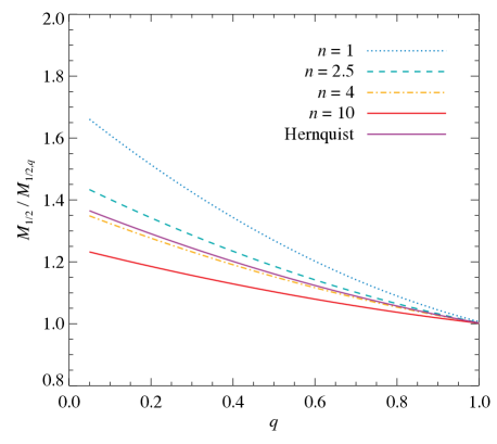
Disc galaxies are not spherically symmetric, so a more useful definition in these cases is the dynamical mass within an oblate spheroid of semi-major axis $r_{1/2}$, which we denote $M_{1/2,\displaystyle q}$. For a given circular velocity, $M_{1/2}>M_{1/2,\displaystyle q}$. This is because the mass that must be spherically distributed to maintain a given circular velocity is larger than that necessary to achieve the same circular velocity in the midplane of a flattened system. The ratio $M_{1/2}/M_{1/2,\displaystyle q}$ is simultaneously a function of the radial profile of the mass distribution and $q$. For a full analytic discussion see, for example, the comparison between the circular velocities of oblate spheroids as a function of $q$ and mass profile in section 2.5.2 of Binney & Tremaine (2008). For our purposes, an approximate estimate of $M_{1/2}/M_{1/2,\displaystyle q}$ is sufficient. Using a range of analytic potentials, we examine the behaviour of the ratio $M_{1/2}/M_{1/2,\displaystyle q}$ as a function of $q$ in Fig. 6. The circular velocity of each flattened model is conveniently calculated numerically by flattening a multi-Gaussian fit to the mass distribution and using standard integrals to determine the circular velocity of the arbitrarily flattened distribution (Cappellari, 2002). Disc galaxies typically have $q\approx 0.2$ and potentials of the form $\exp{(-R/\hbox{$R_{\mathrm{e}}$})^{1/n}}$, where $1\leq n\leq 4$. In such galaxies, $1.3\lesssim M_{1/2}/M_{1/2,\displaystyle q}\lesssim 1.5$, and so from equation (11)

$$M_{1/2,\displaystyle q}\approx r_{1/2}v_{\mathrm{c}}^{2}(r_{1/2})/1.4G.$$ (12)

Furthermore, $r_{1/2}\approx 1.33\hbox{$R_{\mathrm{e}}$}$, where in non-spherical systems the observable $R_{\mathrm{e}}$ is defined as the semi-major axis of the projected half-light ellipse. For disc galaxies we can therefore write

$$M_{1/2,\displaystyle q}\approx\hbox{$R_{\mathrm{e}}$}v_{\mathrm{c}}^{2}(1.33\,\hbox{$R_{\mathrm{e}}$})/G.$$ (13)

The circular velocity at 1.33 $R_{\mathrm{e}}$ can easily be estimated to an accuracy consistent with the derivation of this formula from dynamical modelling, stellar kinematics corrected for asymmetric drift or resolved gas kinematic observations. For typical values of $q$ and the analytic potentials explored here, this expression is accurate to about 15 per cent. Of course in real disc galaxies, the flattening $q$ is a function of radius, the potential is not described by a single Sérsic or Hernquist profile and even $R_{\mathrm{e}}$ is not simple to measure, so equation (13) is probably a little less reliable in practice.

Figure 7: A comparison of the two estimates of the dynamical mass for the 28 galaxies in the present sample. The horizontal axis is $2M_{1/2,\displaystyle q}$ as defined in equation (13), incorporating an approximate correction for flattening. The vertical axis is the $K_{S}$-band luminosity $L$ multiplied by the dynamical mass-to-light ratio $(M/L)_{K_{S},\mathrm{nohalo}}$ as presented in WBC09. The symbols are as in Fig. 2. The solid line is the line $y=x$. The two estimates agree on average to better than 2 per cent with 13 per cent rms scatter and no evidence of a systematic difference between spirals and S0s.

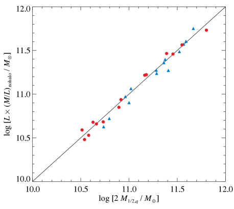
Nevertheless, when doubled, $M_{1/2,\displaystyle q}$ closely matches fiducial estimates of the dynamical mass of our sample galaxies, i.e. the product of their luminosities $L$ and dynamical mass-to-light ratios $(M/L)_{\mathrm{nohalo}}$, inferred in this case from stellar kinematic data extending to 2–3 $R_{\mathrm{e}}$ and $K_{S}$-band photometry in WBC09. We show this comparison in Fig. 7. We use $v_{\mathrm{model}}$, the circular velocity of the WBC09 mass models in the flat region of the observed rotation curve, as $v_{\mathrm{c}}$ in equation (13), but in cases where a reliable asymmetric drift correction is possible at 1.33 $R_{\mathrm{e}}$, $v_{\mathrm{drift}}$ gives almost identical results. The excellent agreement between $2M_{1/2,\displaystyle q}$ and $L\times(M/L)_{\mathrm{nohalo}}$ may be a coincidence. The two measures would be systematically offset (and perhaps more scattered) if our kinematic data extended significantly further in radius (and the dynamical mass-to-light ratios we measured were therefore larger). Crucially, however, Fig. 7 demonstrates that, for the purposes of the present work comparing the TFRs of spirals and S0s, the choice of definition of dynamical mass does not affect spirals and S0s differently.

References

- Aaronson & Mould (1983) Aaronson M., Mould J., 1983, ApJ, 265, 1
- Aguerri et al. (2009) Aguerri J. A. L., Méndez-Abreu J., Corsini E. M., 2009, A&A, 495, 491
- Barway et al. (2009) Barway S., Wadadekar Y., Kembhavi A. K., Mayya Y. D., 2009, MNRAS, 394, 1911
- Baugh (2006) Baugh C. M., 2006, Reports on Progress in Physics, 69, 3101
- Bedregal et al. (2006) Bedregal A. G., Aragón-Salamanca A., Merrifield M. R., 2006, MNRAS, 373, 1125
- Bedregal et al. (2008) Bedregal A. G., Aragón-Salamanca A., Merrifield M. R., Cardiel N., 2008, MNRAS, 387, 660
- Bell & de Jong (2001) Bell E. F., de Jong R. S., 2001, ApJ, 550, 212
- Bertola et al. (1995) Bertola F., Cinzano P., Corsini E. M., Rix H., Zeilinger W. W., 1995, ApJ, 448, L13+
- Binney & Tremaine (2008) Binney J., Tremaine S., 2008, Galactic Dynamics: Second Edition. Princeton University Press
- Blanton & Moustakas (2009) Blanton M. R., Moustakas J., 2009, ARA&A, 47, 159
- Blanton & Roweis (2007) Blanton M. R., Roweis S., 2007, AJ, 133, 734
- Bottinelli et al. (1995) Bottinelli L., Gouguenheim L., Paturel G., Teerikorpi P., 1995, A&A, 296, 64
- Bruzual & Charlot (2003) Bruzual G., Charlot S., 2003, MNRAS, 344, 1000
- Bureau et al. (2006) Bureau M., Aronica G., Athanassoula E., Dettmar R.-J., Bosma A., Freeman K. C., 2006, MNRAS, 370, 753
- Bureau & Freeman (1999) Bureau M., Freeman K. C., 1999, AJ, 118, 126
- Burstein et al. (2005) Burstein D., Ho L. C., Huchra J. P., Macri L. M., 2005, ApJ, 621, 246
- Cappellari (2002) Cappellari M., 2002, MNRAS, 333, 400
- Cappellari (2008) —, 2008, MNRAS, 390, 71
- Cappellari et al. (2006) Cappellari M. et al., 2006, MNRAS, 366, 1126
- Cardelli et al. (1989) Cardelli J. A., Clayton G. C., Mathis J. S., 1989, ApJ, 345, 245
- Chabrier (2003) Chabrier G., 2003, PASP, 115, 763
- Christlein & Zabludoff (2004) Christlein D., Zabludoff A. I., 2004, ApJ, 616, 192
- Chung & Bureau (2004) Chung A., Bureau M., 2004, AJ, 127, 3192
- Chung et al. (2006) Chung A., Koribalski B., Bureau M., van Gorkom J. H., 2006, MNRAS, 370, 1565
- Cinzano et al. (1999) Cinzano P., Rix H., Sarzi M., Corsini E. M., Zeilinger W. W., Bertola F., 1999, MNRAS, 307, 433
- Ciotti (1991) Ciotti L., 1991, A&A, 249, 99
- Conselice et al. (2005) Conselice C. J., Bundy K., Ellis R. S., Brichmann J., Vogt N. P., Phillips A. C., 2005, ApJ, 628, 160
- Corsini et al. (1999) Corsini E. M., Pizzella A., Sarzi M., Cinzano P., Vega Beltrán J. C., Funes J. G., Bertola F., Persic M., Salucci P., 1999, A&A, 342, 671
- Courteau et al. (2007) Courteau S., Dutton A. A., van den Bosch F. C., MacArthur L. A., Dekel A., McIntosh D. H., Dale D. A., 2007, ApJ, 671, 203
- Courteau & Rix (1999) Courteau S., Rix H.-W., 1999, ApJ, 513, 561
- Courtois et al. (2009) Courtois H. M., Tully R. B., Fisher J. R., Bonhomme N., Zavodny M., Barnes A., 2009, AJ, 138, 1938
- Cretton et al. (2000) Cretton N., Rix H., de Zeeuw P. T., 2000, ApJ, 536, 319
- Crook et al. (2007) Crook A. C., Huchra J. P., Martimbeau N., Masters K. L., Jarrett T., Macri L. M., 2007, ApJ, 655, 790
- De Rijcke et al. (2007) De Rijcke S., Zeilinger W. W., Hau G. K. T., Prugniel P., Dejonghe H., 2007, ApJ, 659, 1172
- de Souza & Dos Anjos (1987) de Souza R. E., Dos Anjos S., 1987, A&AS, 70, 465
- de Vaucouleurs et al. (1991) de Vaucouleurs G., de Vaucouleurs A., Corwin H., Buta R., Paturel G., Fouqué P., 1991, Third Reference Catalogue of Bright Galaxies (RC3). Springer-Verlag, Berlin
- Djorgovski & Davis (1987) Djorgovski S., Davis M., 1987, ApJ, 313, 59
- Dressler (1980) Dressler A., 1980, ApJ, 236, 351
- Dressler et al. (1987) Dressler A., Lynden-Bell D., Burstein D., Davies R. L., Faber S. M., Terlevich R., Wegner G., 1987, ApJ, 313, 42
- Dressler et al. (1997) Dressler A., et al., 1997, ApJ, 490, 577
- Dutton et al. (2007) Dutton A. A., van den Bosch F. C., Dekel A., Courteau S., 2007, ApJ, 654, 27
- Emsellem et al. (1994) Emsellem E., Monnet G., Bacon R., 1994, A&A, 285, 723
- Englmaier & Gerhard (1999) Englmaier P., Gerhard O., 1999, MNRAS, 304, 512
- Eskridge et al. (2000) Eskridge P. B. et al. 2000, AJ, 119, 536
- Fasano et al. (2000) Fasano G., Poggianti B. M., Couch W. J., Bettoni D., Kjærgaard P., Moles M., 2000, ApJ, 542, 673
- Flores et al. (2006) Flores H., Hammer F., Puech M., Amram P., Balkowski C., 2006, A&A, 455, 107
- Franx (1993) Franx M., 1993, in IAU Symposium, Vol. 153, Galactic Bulges, H. Dejonghe & H. J. Habing, ed., p. 243
- Freeman (1970) Freeman K. C., 1970, ApJ, 160, 811
- Gerhard et al. (2001) Gerhard O., Kronawitter A., Saglia R. P., Bender R., 2001, AJ, 121, 1936
- Gunn & Gott (1972) Gunn J. E., Gott J. R. I., 1972, ApJ, 176, 1
- Häring & Rix (2004) Häring N., Rix H., 2004, ApJ, 604, L89
- Heald et al. (2007) Heald G. H., Rand R. J., Benjamin R. A., Bershady M. A., 2007, ApJ, 663, 933
- Hernquist (1990) Hernquist L., 1990, ApJ, 356, 359
- Hinz et al. (2003) Hinz J. L., Rieke G. H., Caldwell N., 2003, AJ, 126, 2622
- Hinz et al. (2001) Hinz J. L., Rix H.-W., Bernstein G. M., 2001, AJ, 121, 683
- Hubble (1936) Hubble E. P., 1936, Realm of the Nebulae. Yale University Press
- Jarrett et al. (2000) Jarrett T. H., Chester T., Cutri R., Schneider S., Skrutskie M., Huchra J. P., 2000, AJ, 119, 2498
- Jarvis (1986) Jarvis B. J., 1986, AJ, 91, 65
- Jeans (1922) Jeans J. H., 1922, MNRAS, 82, 122
- Jensen et al. (2003) Jensen J. B., Tonry J. L., Barris B. J., Thompson R. I., Liu M. C., Rieke M. J., Ajhar E. A., Blakeslee J. P., 2003, ApJ, 583, 712
- Jeong et al. (2009) Jeong H. et al., 2009, MNRAS, 398, 2028
- Karachentsev et al. (1993) Karachentsev I. D., Karachentseva V. E., Parnovskij S. L., 1993, Astronomische Nachrichten, 314, 97
- Kassin et al. (2006) Kassin S. A., de Jong R. S., Weiner B. J., 2006, ApJ, 643, 804
- Kassin et al. (2007) Kassin S. A. et al., ApJ, 660, L35
- Kaviraj et al. (2007) Kaviraj S., Schawinski K., Devriendt J. E. G., et al., 2007, ApJS, 173, 619
- Kent (1988) Kent S. M., 1988, AJ, 96, 514
- Koen & Lombard (2009) Koen C., Lombard F., 2009, MNRAS, 395, 1657
- Komatsu et al. (2009) Komatsu E., et al., 2009, ApJS, 180, 330
- Kormendy & Westpfahl (1989) Kormendy J., Westpfahl D. J., 1989, ApJ, 338, 752
- Krajnović et al. (2005) Krajnović D., Cappellari M., Emsellem E., McDermid R. M., de Zeeuw P. T., 2005, MNRAS, 357, 1113
- Kuijken & Merrifield (1995) Kuijken K., Merrifield M. R., 1995, ApJL, 443, L13
- Larson et al. (1980) Larson R. B., Tinsley B. M., Caldwell C. N., 1980, ApJ, 237, 692
- Laurikainen et al. (2009) Laurikainen E., Salo H., Buta R., Knapen J. H., 2009, ApJ, 692, L34
- Levine et al. (2008) Levine E. S., Heiles C., Blitz L., 2008, ApJ, 679, 1288
- Macciò et al. (2008) Macciò A. V., Dutton A. A., van den Bosch F. C., 2008, MNRAS, 391, 1940
- Magorrian & Ballantyne (2001) Magorrian J., Ballantyne D., 2001, MNRAS, 322, 702
- Magorrian et al. (1998) Magorrian J., Tremaine S., Richstone D., Bender R., Bower G., Dressler A., Faber S. M., Gebhardt K., Green R., Grillmair C., Kormendy J., Lauer T., 1998, AJ, 115, 2285
- Marigo & Girardi (2007) Marigo P., Girardi L., 2007, A&A, 469, 239
- Marinova & Jogee (2007) Marinova I., Jogee S., 2007, ApJ, 659, 1176
- Markwardt (2008) Markwardt C. B., 2008, in Astronomical Data Analysis Software and Systems XVIII, Bohlender, D., Dowler P., Durand D., eds., Astronomical Society of the Pacific Conference Series
- Masters et al. (2008) Masters K. L., Springob C. M., Huchra J. P., 2008, AJ, 135, 1738
- Mathieu et al. (2002) Mathieu A., Merrifield M. R., Kuijken K., 2002, MNRAS, 330, 251
- McGaugh et al. (2000) McGaugh S. S., Schombert J. M., Bothun G. D., de Blok W. J. G., 2000, ApJ, 533, L99
- Mehlert et al. (2003) Mehlert D., Thomas D., Saglia R. P., Bender R., Wegner G., 2003, A&A, 407, 423
- Mei et al. (2007) Mei S., et al., 2007, ApJ, 655, 144
- Merrifield & Kuijken (1999) Merrifield M. R., Kuijken K., 1999, A&A, 345, L47
- Merrifield et al. (2010) Merrifield M. R., et al., 2010, in Hunting for the Dark: The Hidden Side of Galaxy Formation, Debattista V. P., Popescu C. C., eds., AIP Conf. Ser.
- Moore et al. (1996) Moore B., Katz N., Lake G., Dressler A., Oemler A., 1996, Nature, 379, 613
- Mould et al. (2000) Mould J. R. et al., 2000, ApJ, 529, 786
- Navarro et al. (1997) Navarro J. F., Frenk C. S., White S. D. M., 1997, ApJ, 490, 493
- Neistein et al. (1999) Neistein E., Maoz D., Rix H.-W., Tonry J. L., 1999, AJ, 117, 2666
- Noordermeer et al. (2007) Noordermeer E., van der Hulst J. M., Sancisi R., Swaters R. S., van Albada T. S., 2007, MNRAS, 376, 1513
- Noordermeer & Verheijen (2007) Noordermeer E., Verheijen M. A. W., 2007, MNRAS, 381, 1463
- Noordermeer et al. (2008) Noordermeer E., et al., 2008, MNRAS, 384, 943
- Oosterloo et al. (2007) Oosterloo T., Fraternali F., Sancisi R., 2007, AJ, 134, 1019
- Palunas & Williams (2000) Palunas P., Williams T. B., 2000, AJ, 120, 2884
- Paturel et al. (2003) Paturel G., Petit C., Prugniel P., Theureau G., Rousseau J., Brouty M., Dubois P., Cambrésy L., 2003, A&A, 412, 45
- Peletier & Willner (1993) Peletier R. F., Willner S. P., 1993, ApJ, 418, 626
- Persic et al. (1996) Persic M., Salucci P., Stel F., 1996, MNRAS, 281, 27
- Pizagno et al. (2007) Pizagno J., Prada F., Weinberg D. H., Rix H.-W., Pogge R. W., Grebel E. K., Harbeck D., Blanton M., Brinkmann J., Gunn J. E., 2007, AJ, 134, 945
- Pizzella et al. (2004) Pizzella A., Corsini E. M., Vega Beltrán J. C., Bertola F., 2004, A&A, 424, 447
- Poggianti et al. (2001) Poggianti B. M., et al., 2001, ApJ, 563, 118
- Puech et al. (2008) Puech M., et al., 2008, A&A, 484, 173
- Roberts (1978) Roberts M. S., 1978, AJ, 83, 1026
- Rothberg et al. (2000) Rothberg B., Saunders W., Tully R. B., Witchalls P. L., 2000, ApJ, 533, 781
- Rubin et al. (1985) Rubin V. C., Burstein D., Ford Jr. W. K., Thonnard N., 1985, ApJ, 289, 81
- Sakai et al. (2000) Sakai S., et al., 2000, ApJ, 529, 698
- Sandage (1961) Sandage A., 1961, The Hubble Atlas of Galaxies. Washington: Carnegie Institution, 1961
- Schlegel et al. (1998) Schlegel D. J., Finkbeiner D. P., Davis M., 1998, ApJ, 500, 525
- Shapiro et al. (2010) Shapiro K. L. et al., 2010, MNRAS, 402, 2140
- Shaw (1987) Shaw M. A., 1987, MNRAS, 229, 691
- Singhal (2008) Singhal A., 2008, PhD thesis, University of Virginia
- Spitzer & Baade (1951) Spitzer L. J., Baade W., 1951, ApJ, 113, 413
- Stark et al. (2009) Stark D. V., McGaugh S. S., Swaters R. A., 2009, AJ, 138, 392
- Temi et al. (2009a) Temi P., Brighenti F., Mathews W. G., 2009a, ApJ, 695, 1
- Temi et al. (2009b) —, 2009b, ApJ, 707, 890
- Thomas et al. (2009) Thomas J., Jesseit R., Saglia R. P., Bender R., Burkert A., Corsini E. M., Gebhardt K., Magorrian J., Naab T., Thomas D., Wegner G., 2009, MNRAS, 393, 641
- Tonini et al. (2010) Tonini C., Maraston C., Ziegler B., Böhm A., Thomas D., Devriendt J., Silk J., 2010, MNRAS (submitted, arXiv:1006.0229)
- Tonry et al. (2000) Tonry J. L., Blakeslee J. P., Ajhar E. A., Dressler A., 2000, ApJ, 530, 625
- Tonry et al. (2001) Tonry J. L., Dressler A., Blakeslee J. P., Ajhar E. A., Fletcher A. B., Luppino G. A., Metzger M. R., Moore C. B., 2001, ApJ, 546, 681
- Tremaine et al. (2002) Tremaine S. et al., 2002, ApJ, 574, 740
- Trujillo-Gomez et al. (2010) Trujillo-Gomez S., Klypin A., Primack J., Romanowsky A. J., 2010, AJ (submitted, arXiv:1005.1289)
- Tully & Fisher (1977) Tully R. B., Fisher J. R., 1977, A&A, 54, 661
- Tully & Fouqué (1985) Tully R. B., Fouqué P., 1985, ApJS, 58, 67
- Tully et al. (1982) Tully R. B., Mould J. R., Aaronson M., 1982, ApJ, 257, 527
- Tully & Pierce (2000) Tully R. B., Pierce M. J., 2000, ApJ, 533, 744
- van Albada et al. (1985) van Albada T. S., Bahcall J. N., Begeman K., Sancisi R., 1985, ApJ, 295, 305
- van Albada & Sancisi (1986) van Albada T. S., Sancisi R., 1986, Royal Society of London Philosophical Transactions Series A, 320, 447
- van den Bergh (2009) van den Bergh S., 2009, ApJ, 702, 1502
- Vega Beltrán et al. (2001) Vega Beltrán J. C., Pizzella A., Corsini E. M., Funes J. G., Zeilinger W. W., Beckman J. E., Bertola F., 2001, A&A, 374, 394
- Verheijen (2001) Verheijen M. A. W., 2001, ApJ, 563, 694
- Weijmans et al. (2008) Weijmans A.-M., Krajnović D., van de Ven G., Oosterloo T. A., Morganti R., de Zeeuw P. T., 2008, MNRAS, 383, 1343
- Weiner et al. (2001) Weiner B. J., Sellwood J. A., Williams T. B., 2001, ApJ, 546, 931
- Whyte et al. (2002) Whyte L. F., Abraham R. G., Merrifield M. R., Eskridge P. B., Frogel J. A., Pogge R. W., 2002, MNRAS, 336, 1281
- Williams et al. (2009) Williams M. J., Bureau M., Cappellari M., 2009, MNRAS, 400, 1665
- Willick (1994) Willick J. A., 1994, ApJS, 92, 1
- Wilman et al. (2009) Wilman D. J., Oemler A., Mulchaey J. S., McGee S. L., Balogh M. L., Bower R. G., 2009, ApJ, 692, 298
- Wolf et al. (2010) Wolf J., Martinez G. D., Bullock J. S., Kaplinghat M., Geha M., Muñoz R. R., Simon J. D., Avedo F. F., 2010, MNRAS, 406, 1220
- Young et al. (2008) Young L. M., Bureau M., Cappellari M., 2008, ApJ, 676, 317