The Evolution of Lyman Limit Absorption Systems to Redshift Six**affiliation: Based in part on data obtained from the Multimission Archive at the Space Telescope Science Institute (MAST). STScI is operated by the Association of Universities for Research in Astronomy, Inc., under NASA contract NAS5–26555. Support for MAST for non-HST data is provided by the NASA Office of Space Science via grant NAG5–7584 and by other grants and contracts.
Abstract
We have measured the redshift evolution of the density of Lyman limit systems (LLS) in the intergalactic medium over the redshift range . We have used two new quasar samples to (1) improve coverage at , with GALEX grism spectrograph observations of 50 quasars with , and (2) extend coverage to , with Keck ESI spectra of 25 quasars with . Using these samples together with published data, we find that the number density of LLS per unit redshift, , can be well fit by a simple evolution of the form with and for the entire range . We have also reanalyzed the evolution of damped Lyman alpha systems (DLAs) in the redshift range using our high-redshift quasar sample. We find a total of 17 DLAs and sub-DLAs, which we have analyzed in combination with published data. The DLAs with show the same redshift evolution as the LLS. When combined with previous results, our DLA sample is also consistent with a constant from to . We have used the LLS number density evolution to compute the evolution in the mean free path of ionizing photons. We find a smooth evolution to , very similar in shape to that of Madau, Haardt & Rees (1999) but about a factor of two higher. Recent theoretical models roughly match to the data but diverge from the measured power law at in different ways, cautioning against extrapolating the fit to the mean free path outside the measured redshift range.
Subject headings:
cosmology: observations — early universe — quasars: absorption lines — galaxies: evolution — galaxies: formation1. Introduction
Intergalactic absorption lines that are optically thick to radiation at the Lyman continuum edge are generally referred to as Lyman limit systems (LLS). The LLS are perhaps the single most valuable tracer of the evolution of the intergalactic medium since they provide a nearly direct measure of the mean free path of ionizing radiation at high redshifts. They are therefore a key ingredient in estimating the required sources of ionizing radiation needed to maintain the ionization in the intergalactic gas (Madau, Haardt & Rees, 1999 [MHR]). The expected rapid positive evolution in the number of such systems as the intergalactic gas becomes more opaque means that they could, in principle, be an indicator of the approach of the epoch of reionization.
LLS are also the easiest systems to identify in quasar spectra since the abrupt break in the spectrum produced by the absorption systems can easily be seen in relatively noisy and low resolution observations. Since Tytler’s pioneering work on the cosmological evolution of the LLS (Tytler 1982), numerous groups have measured LLS evolution over a range of redshifts extending from low redshift systems, measured with HST, to (Bechtold et al. 2002; Sargent, Steidel & Boksenberg 1989 [SSB]; Lanzetta 1991; Storrie-Lombardi et al. 1994; Stengler-Larrea et al. 1995 [SL95]; Lanzetta et al. 1995; Péroux 2001; Péroux et al. 2003 [P03]). The simplicity of identifying LLS means that we can extend this type of measurement yet further, out to , and this is the primary goal of the present paper. Indeed LLS are the only neutral hydrogen line systems that we can readily trace beyond . At these high redshifts, the lower column density Ly forest is too blended and the quasar continuum too ill-defined for these systems to be studied, and we can no longer determine the radiation damping wings that allow us to identify the stronger systems such as the damped Ly aborbers (DLAs). The LLS are therefore the one way we have to normalize the neutral hydrogen column density function at these redshifts, a crucial input to any modelling of the intergalactic medium.
| QSO | Exp (hr) | Ref.a | ||||||
|---|---|---|---|---|---|---|---|---|
| FIRS0747+2739 | 4.17000 | 4.42 | 3.4228 | 20.80 | 20.85 (PW) | |||
| 3.9012 | 20.50 | 20.50 (PW) | ||||||
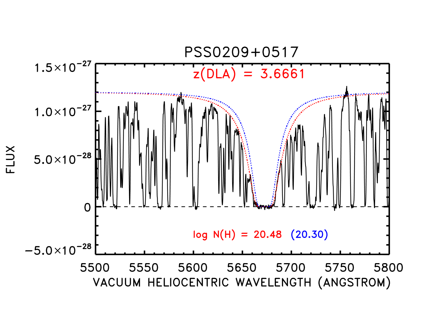
| PSS0209+0517 | 4.17000 | 3.00 | 3.99060 | 4.6 | 3.98828 | 3.6661 | 20.48 | 20.45 (PW) |
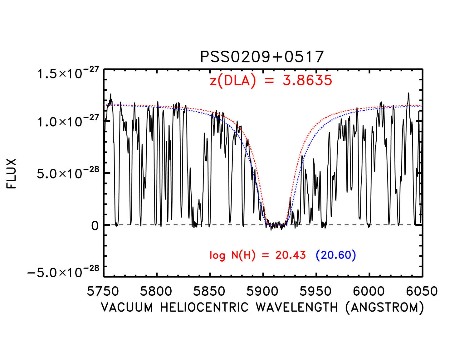
| 3.8635 | 20.43 | 20.55 (PW) | ||||||
| PSS0926+3055 | 4.19000 | 3.00 | ||||||
| BRJ04262202 | 4.32000 | 3.00 | ||||||
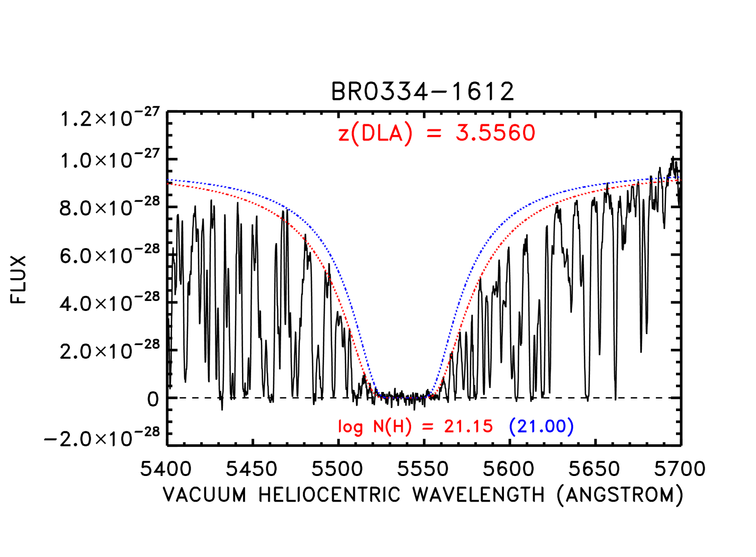
| BR03341612 | 4.36300 | 3.00 | 4.23037 | 2.8 | 4.23454 | 3.556 | 21.15 | 21.0 (P03) |
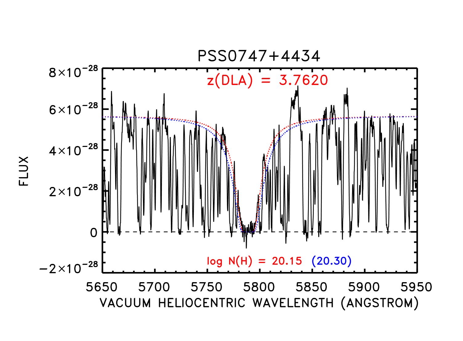
| PSS0747+4434 | 4.39000 | 3.00 | 4.29520 | 1.1 | 4.27546 | 3.762 | 20.15 | 20.3 (P03) |
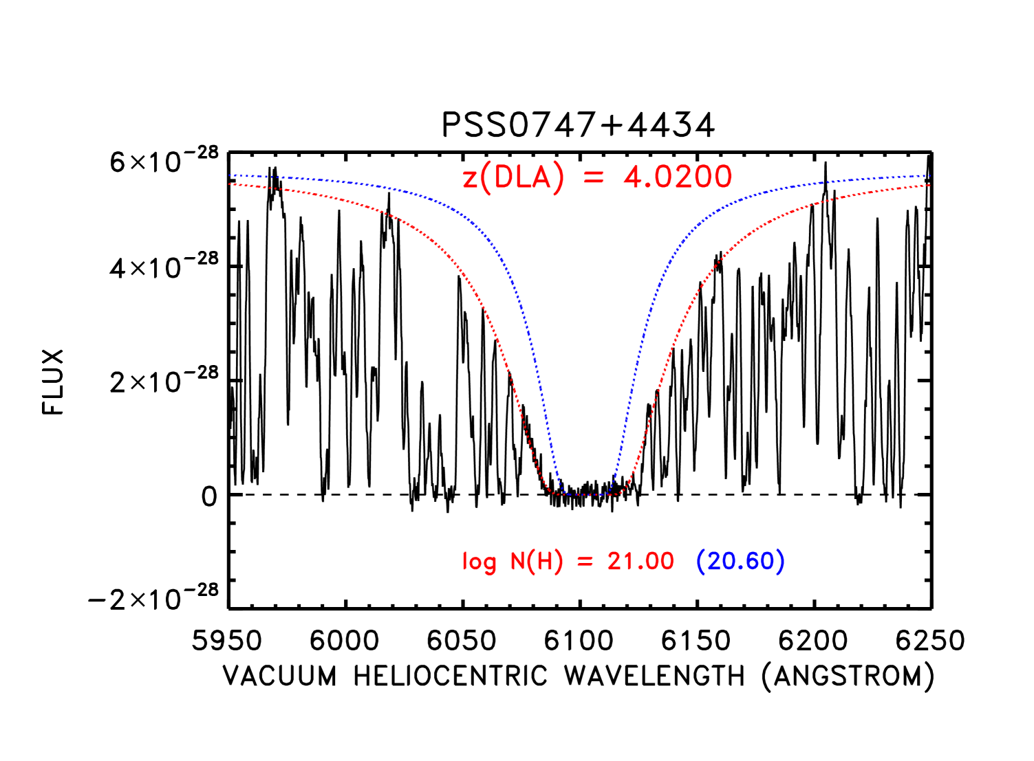
| 4.020 | 21.0 | 20.6 (P03) | ||||||
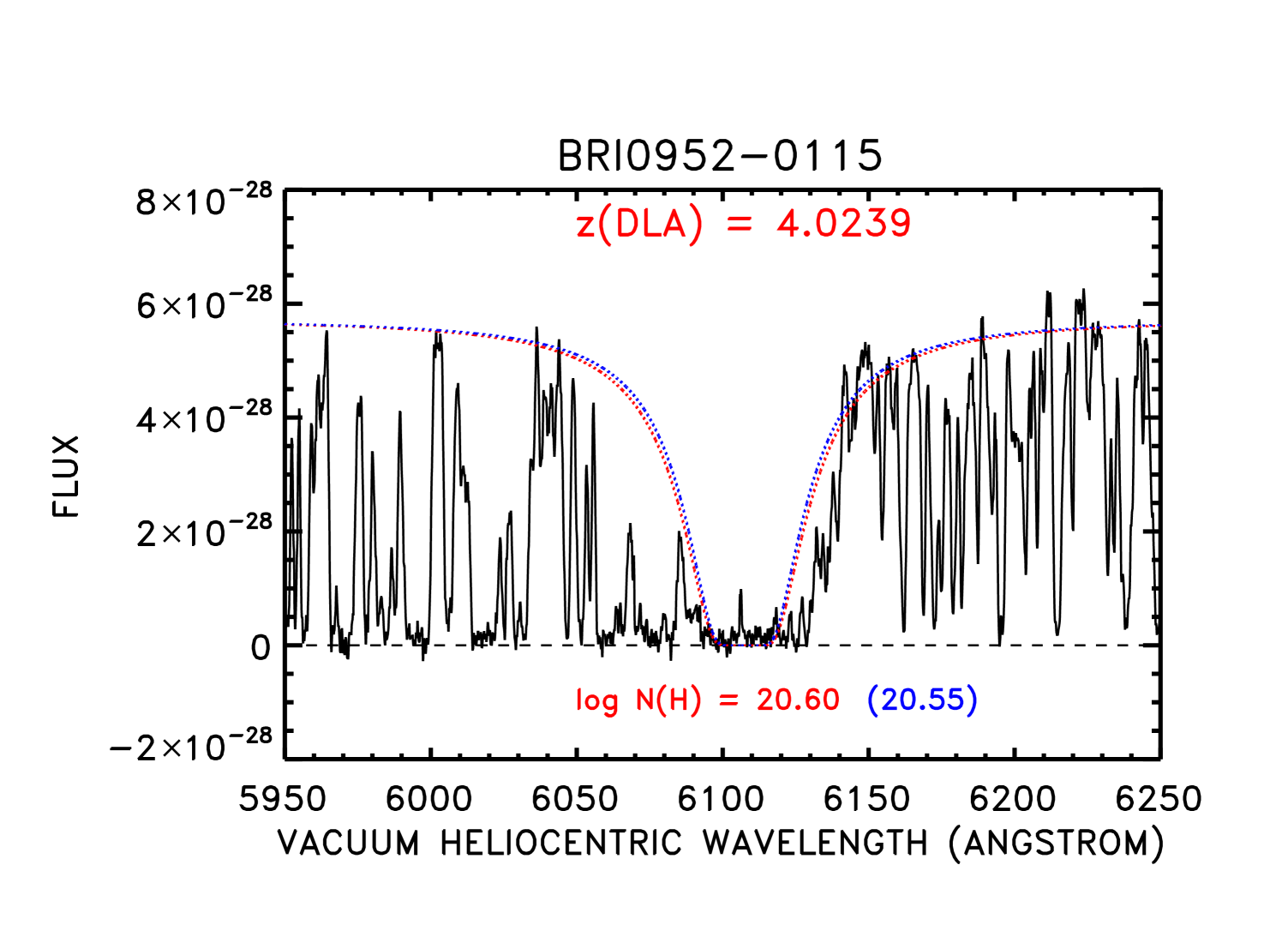
| BRI09520115 | 4.42000 | 4.25 | 4.37745 | 1.1 | 4.37813 | 4.0239 | 20.60 | 20.55 (PW) |
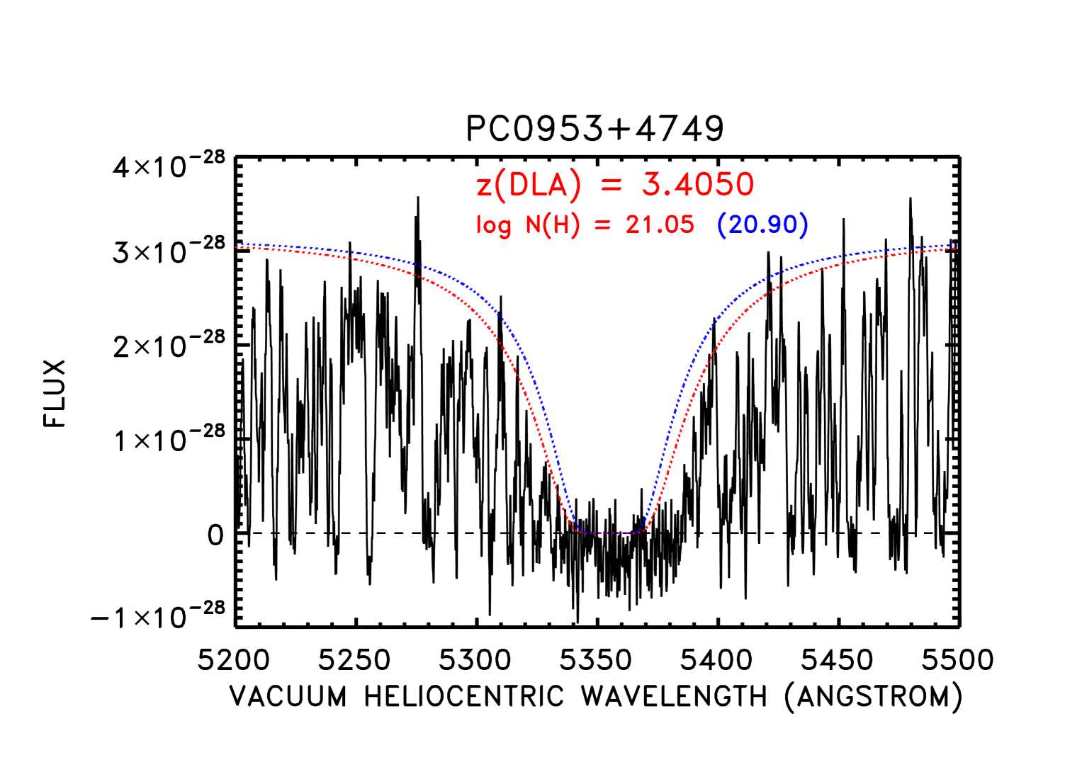
| PC0953+4749 | 4.46000 | 2.00 | 4.32691 | 4.34002 | 3.405 | 21.05 | 21.15 (PW) | |
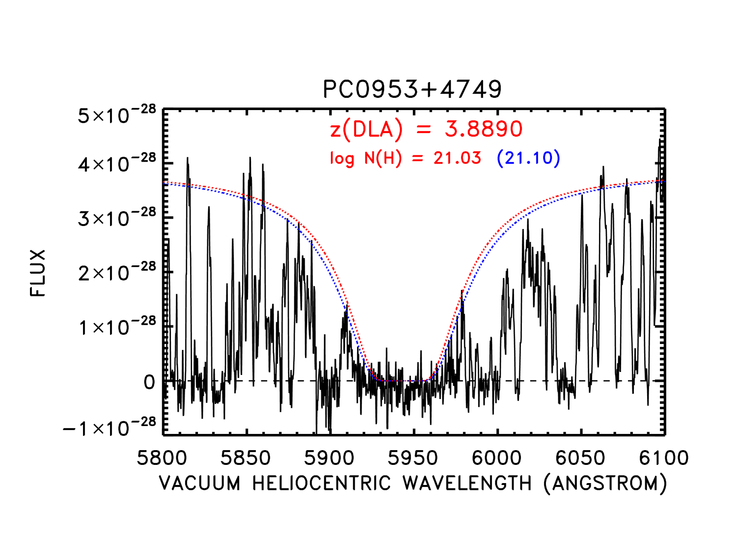
| 3.889 | 21.03 | 21.20 (PW) | ||||||
| 4.2444 | 20.95 | 20.90 (PW) | ||||||
| BR10330327 | 4.51000 | 2.00 | 4.18764 | 4.17502 | 4.174 | 20.08 | ||
| BR22370607 | 4.55000 | 11.56 | 4.25832 | 4.24740 | 4.080 | 20.53 | 20.52 (PW) | |
| PSS1347+4956 | 4.56500 | 1.20 | 4.28753 | 1.9 | 4.27248 | |||
| BR03533820 | 4.58000 | 2.50 | 4.36619 | 1.5 | 4.35953 | |||
| BR12020725 | 4.61000 | 3.00 | 4.48567 | 4.48012 | 4.383 | 20.62 | 20.60 (PW) | |
| SDSS2200+0017 | 4.78000 | 6.83 | 4.62166 | 4.65974 | ||||
| SDSS0206+1216 | 4.81000 | 3.00 | 4.34606 | 4.32516 | 4.3255 | 20.78 | ||
| SDSS1737+5828 | 4.85000 | 9.00 | 4.74902 | 4.74314 | 4.7415 | 20.70 | 20.65 (PW) | |
| SDSS02110009 | 4.90000 | 6.00 | 4.67670 | 4.64357 | 4.644 | 20.18 | ||
| SDSS0338+0021 | 5.01000 | 7.25 | 4.97626 | 1.7 | 4.97778 | |||
| SDSS12040021 | 5.07000 | 3.00 | ||||||
| SDSS02310728 | 5.42000 | 4.33 | 5.40306 | 5.38874 | ||||
| SDSS10440125 | 5.74500 | 5.75 | 5.64344 | |||||
| SDSS0002+2550 | 5.80000 | 5.75 | 5.72026 | |||||
| SDSS0836+0054 | 5.82000 | 11.83 | 5.47923 | |||||
| SDSS1411+1217 | 5.93000 | 6.50 | 5.89278 | 2.3 | 5.89602 | |||
| SDSS1306+0356 | 5.99000 | 9.75 | 5.97264 | 2.6 |
In the present paper we combine data on the LLS from a high redshift () sample with a new low redshift sample () and with pre-existing observations at intermediate redshifts to compute the evolution of the LLS over the redshift interval . The high redshift sample is based on high signal to noise obervations of a sample of 25 quasars (section 2.1). The new sample is based on a large sample of quasars selected from grism spectra taken with the GALEX satellite. We use this to reinvestigate the low redshift density of LLS since the GALEX sample should be more homogeneous and unbiased than the previous HST and IUE samples used for this purpose. We find a lower value for the LLS density at this redshift with the new sample. Remarkably we find that the evolution over the full reshift range can be fit by a single power law of the form and that this extends smoothly to near , beyond which the Lyman forest portions of the quasar spectra become too opaque to continue the measurement.
We have also measured the DLAs () and sub-DLAs (here defined as ) at in our high-redshift quasar sample, and used these in combination with previous work to test if the form of the neutral hydrogen column density distribution is changing as a function of redshift. The combined data are consistent with an invariant form of the function.
We also compute the neutral hydrogen density in the range and find that is invariant over the redshift range . The LLS density evolution implies that this result may extend to if the neutral hydrogen column density distribution function remains invariant.
We use the form of the LLS evolution to compute the mean free path for ionizing photons, showing that the present observations decrease this compared with recent analyses (e.g. Faucher-Giguère et al. 2008). Finally we compare the evolution of the LLS and the mean free path to recent theoretical models. We assume , and throughout.
| QSO | R.A. (J2000.0) | Decl. (J2000.0) | ||
|---|---|---|---|---|
| GALEX1713+6001 | 258.29000 | + 60.024200 | 0.8179 | |
| GALEX1238+6143 | 189.70300 | + 61.73180 | 0.8323 | |
| GALEX1438+3446 | 219.54100 | + 34.76800 | 0.8331 | |
| GALEX1050+5819 | 162.50100 | + 58.31790 | 0.8350 | |
| GALEX1421+5241 | 215.30099 | + 52.69649 | 0.8438 | |
| GALEX1436+3539 | 219.17599 | + 35.65800 | 0.8450 | |
| GALEX0040-4403 | 10.17800 | 0.8524 | 0.7784 | |
| GALEX0040-4340 | 10.11710 | 0.8726 | ||
| GALEX1434+3529 | 218.68699 | + 35.48809 | 0.8729 | |
| GALEX1437+3508 | 219.25599 | + 35.13760 | 0.8800 | |
| GALEX1237+6211 | 189.49800 | + 62.18399 | 0.9129 | |
| GALEX1051+5838 | 162.77200 | + 58.64239 | 0.9150 | |
| GALEX1434+3456 | 218.69799 | + 34.93420 | 0.9269 | 0.8864 |
| GALEX0038-4352 | 9.53954 | 0.9359 | ||
| GALEX1052+5851 | 163.072998 | + 58.85630 | 0.9700 | |
| GALEX1001+0200 | 150.46299 | + 2.0090301 | 0.9705 | |
| GALEX1417+5230 | 214.39999 | + 52.50840 | 0.9877 | |
| GALEX0333-2817 | 53.41400 | 0.9906 | ||
| GALEX1723+5951 | 260.79299 | + 59.85160 | 0.9964 | 0.7935 |
| GALEX1238+6202 | 189.56700 | + 62.0356 | 0.9976 | |
| GALEX1423+5246 | 215.76699 | + 52.77500 | 0.9993 | |
| GALEX1712+6005 | 258.14498 | + 60.091800 | 0.9993 | |
| GALEX1237+6217 | 189.27900 | + 62.28400 | 1.0190 | |
| GALEX0334-2743 | 53.53450 | 1.0281 | ||
| GALEX0332-2740 | 53.11040 | 1.0396 | ||
| GALEX1717+5947 | 259.38699 | + 59.79650 | 1.0482 | |
| GALEX1420+5216 | 215.035003 | + 52.27980 | 1.0600 | |
| GALEX1719+6013 | 259.96398 | + 60.22259 | 1.0600 | |
| GALEX1436+3525 | 219.10299 | + 35.42699 | 1.0648 | |
| GALEX1436+3453 | 219.13200 | + 34.89020 | 1.0676 | |
| GALEX1724+5921 | 261.21398 | + 59.35920 | 1.0770 | 0.7770 |
| GALEX1436+3537 | 219.074005 | + 35.62390 | 1.0776 | 0.8428 |
| GALEX1240+6223 | 190.13900 | + 62.39090 | 1.1115 | |
| GALEX1437+3442 | 219.43200 | + 34.71490 | 1.1146 | |
| GALEX1435+3457 | 218.78199 | + 34.95679 | 1.1174 | |
| GALEX1418+5223 | 214.66000 | + 52.39989 | 1.1202 | 1.1100 |
| GALEX1234+6233 | 188.50500 | + 62.55410 | 1.1231 | |
| GALEX0333-2725 | 53.35220 | 1.1400 | ||
| GALEX1435+3504 | 218.86799 | + 35.075801 | 1.1472 | |
| GALEX1418+5252 | 214.50700 | + 52.86690 | 1.1600 | |
| GALEX0334-2745 | 53.57030 | 1.1634 | 0.8325 | |
| GALEX1720+5932 | 260.13501 | + 59.53530 | 1.1691 | |
| GALEX1002+0230 | 150.54499 | + 2.50739 | 1.1691 | 0.7651 |
| GALEX1053+5855 | 163.29200 | + 58.92580 | 1.1800 | |
| GALEX1054+5852 | 163.58700 | + 58.87179 | 1.1835 | |
| GALEX1239+6206 | 189.88099 | + 62.10520 | 1.2008 | |
| GALEX1712+6007 | 258.13198 | + 60.12210 | 1.2037 | 0.8201 |
| GALEX1416+5259 | 214.20100 | + 52.98410 | 1.2325 | |
| GALEX0040-4409 | 10.24390 | 1.2325 | ||
| GALEX1419+5232 | 214.94299 | + 52.54639 | 1.2469 |
2. Data
2.1. High redshift quasars
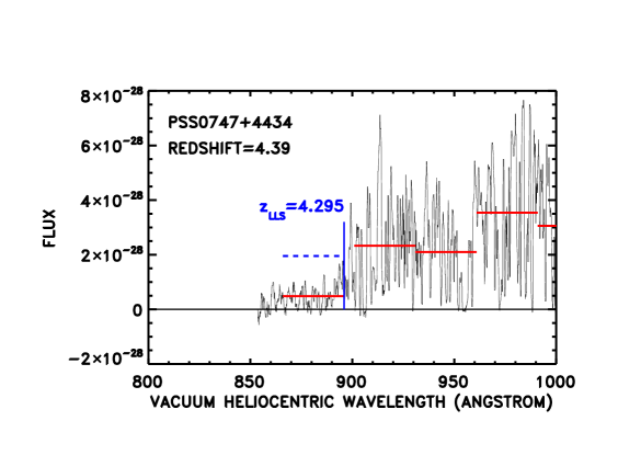
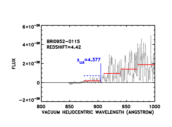
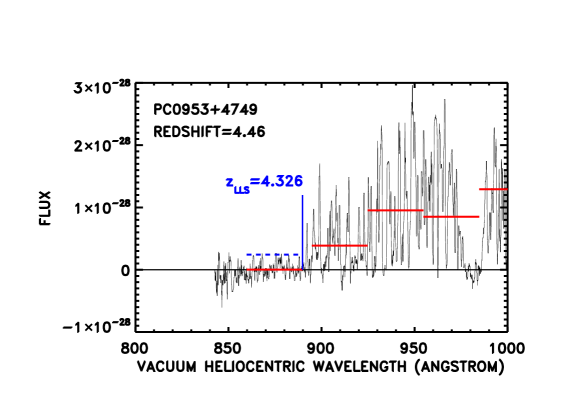
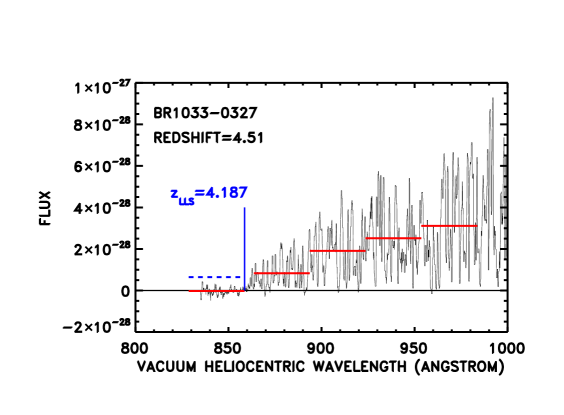
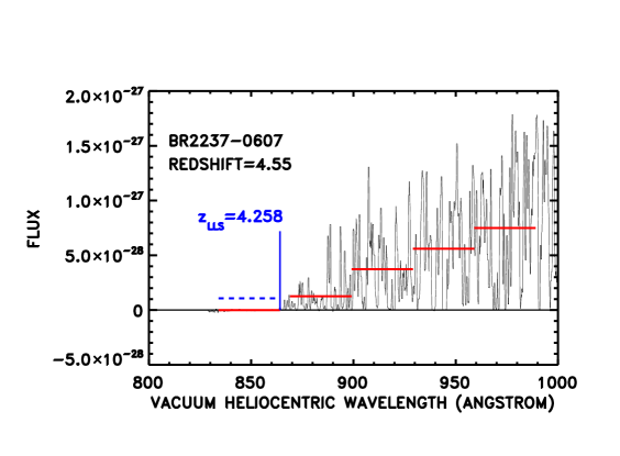
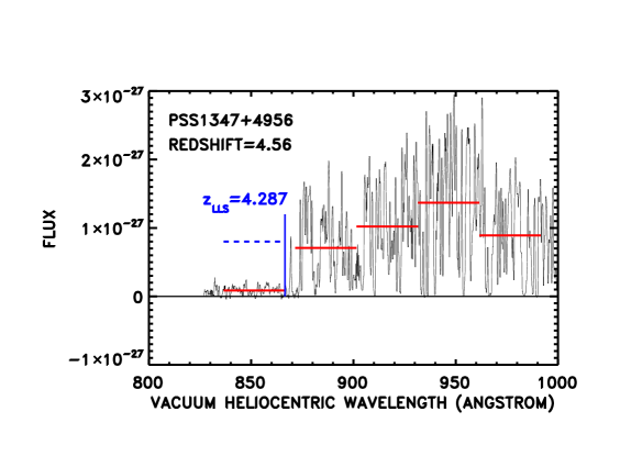
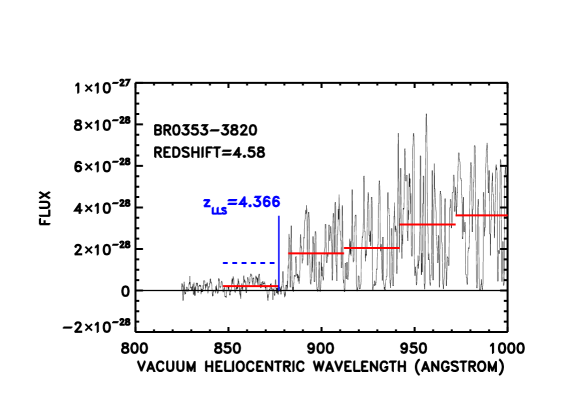
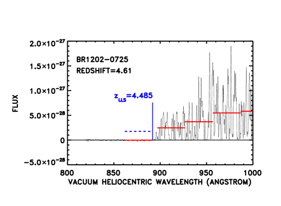
We used a data set (Table 1) consisting of spectra of 25 quasars selected to span the redshift range from . The sample was chosen from among the brightest quasars at these redshifts based only on accessibility at the time of the observations. One additional BALQSO was observed in the program but has been eliminated from the present sample. While color-based quasar selection can introduce a bias toward quasars with strong LLS at lower redshifts, the L forest is sufficiently strong at these redshifts to ensure that the quasars would be picked out irrespective of the presence of an LLS (see Péroux 2001). The spectra were taken on the Keck II telescope with the ESI instrument in echellette mode with exposure times ranging from just under 2 hours to just under 12 hours. The resolution in this configuration is comparatively low, for the slit width used, but the red sensitivity is high and the wavelength coverage is complete from to . At the red wavelengths, precision sky subtraction is required since the sky lines can be more than two orders of magnitude brighter than the quasars. In order to deal with this issue, individual half-hour exposures were made, stepped along the slit, and the median was used to provide the primary sky subtraction. The frames were then registered, filtered to remove cosmic rays and artifacts, and then added. At this point a second linear fit to the slit profile in the vicinity of the quasar was used to remove any small residual sky. This procedure gives an extremely accurate sky subtraction and a precise zero level in the spectra. The observations were made at the parallactic angle and flux calibrated using observations of white dwarf standards scattered through the night. These standards were also used to remove telluric absorption features in the spectra, including the various atmospheric bands. The final extractions of the spectra were made using a weighting provided by the profile of the white dwarf standards. Wavelength calibrations were obtained using third-order fits to CuAr and Xe lamp observations at the begining and end of each night, and the absolute wavelength scale was then obtained by registering these wavelength solutions to the night sky lines. The wavelengths and redshifts are given in the vacuum heliocentric frame. A sample of the final spectra of the 25 quasars is shown in Figure 11 and all of the spectra are given in the Appendix.

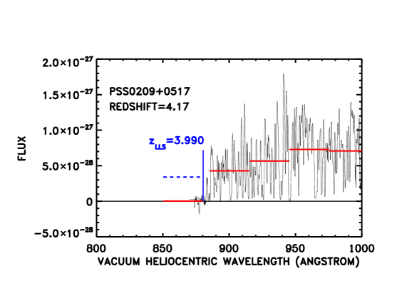
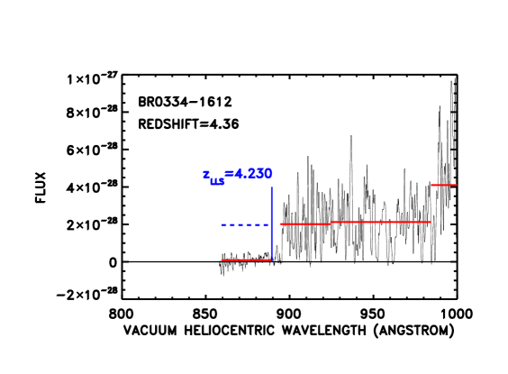
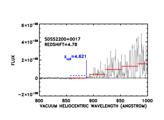
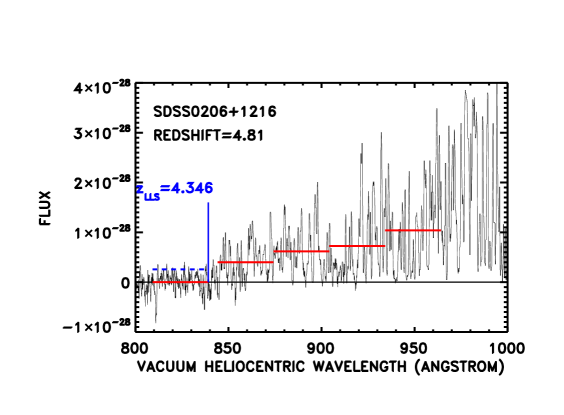
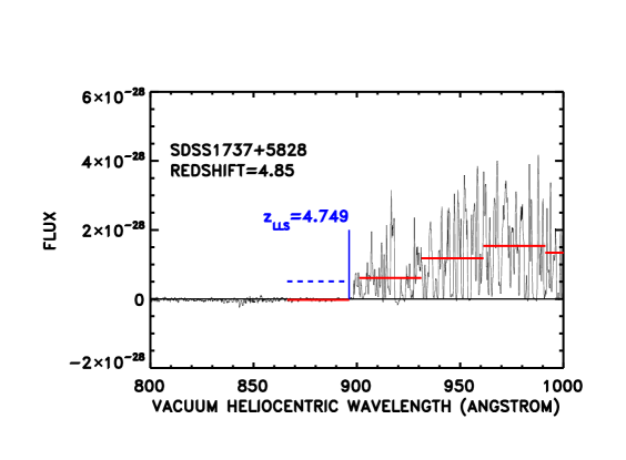
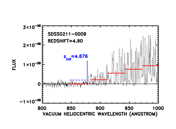
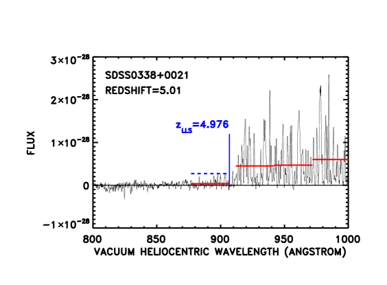
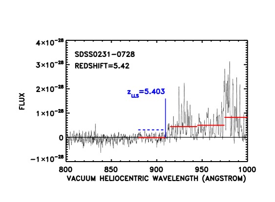
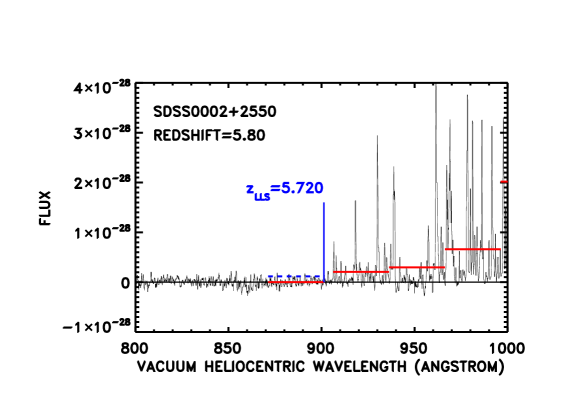
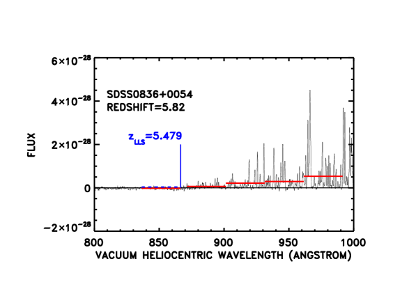
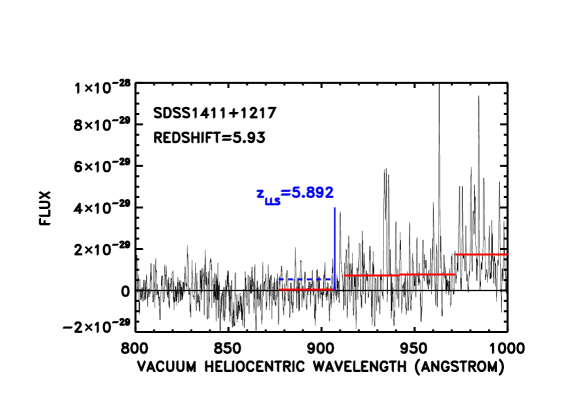
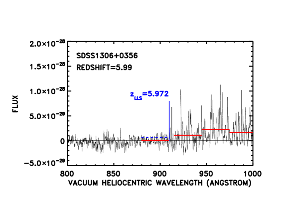
Each spectrum was visually inspected to determine the wavelength () below which the spectrum dropped by more than a factor of 2.7 (). We adopt the redshift as the Lyman limit redshift. The procedure used is shown in Figure 2 (see also Appendix) where we plot the quasar spectra in the vicinity of the LLS and show the average fluxes in wavelength intervals above and below the position of the LLS. The results are summarized in Table 1, where we give the quasar name, its emission redshift , the ESI exposure time and the LLS redshift (columns 1 – 4). Where no LLS is detected to our adopted wavelength limit of () we show a blank entry in Table 1. For each Lyman limit system we searched for corresponding metal-line absorption and where this was detected we also give the metal-line redshift (column 6). The optical depth was now measured by computing the actual flux for a rest frame interval of immediately below the LLS wavelength and taking the log of the ratio of this quantity to the flux obtained by extrapolating a power-law fit to the quasar spectrum at 10 – longward of the LLS, excluding the region around the O VI + Ly quasar emission. The procedure is illustrated in Figure 2 and the optical depths are tabulated in column 5 of Table 1.
We tested the accuracy of the LLS redshift determinations and optical depth measurements by simulating LLS in the spectra and then measuring the recovered redshift and optical depth. For each quasar for which there was sufficient wavelength space between the first real LLS and the quasar L emission line, we inserted a false LLS at a randomly generated wavelength and with a specified optical depth. Below the wavelength of the false LLS we added in artificial noise matched to the quasar exposure time. We then remeasured the LLS redshift and optical depth using our standard procedure. We repeated this twenty times for each quasar for three optical depths: , 1.5 and 2.0.
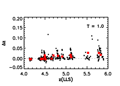
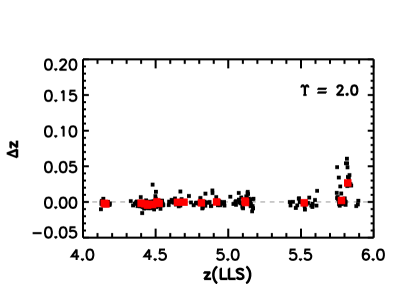
The measured redshift offset as a function of LLS redshift is shown in Figure 3 for and 2.0. In both cases we have shown the individual offsets of each simulation with smaller symbols, and the average in a particular quasar with the larger symbol. As would be expected, offsets tend to be positive, i.e. the measured redshift is very slightly higher than the real one. This is a consequence of blending with the forest. The effect is larger for lower optical depth and at higher redshift, where the forest becomes richer. Typical offsets in the case where the effect is largest are below , rising to – 0.03 in the highest redshift quasars. The errors are generally smaller for the systems. We shall consider the systematic errors which can be introduced by these offsets in the next section. However, the systematic errors introduced by the redshift uncertainty are smaller than the statistical uncertainty. We also used the simulation to calibrate the measurements of the optical depth and examine the systematic errors in the determination of this quantity. We find that the errors are dominated by the continuum fitting, with a dispersion of 0.3 in , and that there is a systematic offset of in . This is introduced by the use of a single power law fit which systematically overestimates the continuum. We have corrected the values of given in Table 1 to allow for this offset. The statistical errors and other systematic errors are completely dominated by the continuum fitting error. We consider the effects of the continuum fitting error on the determination of the LLS number density in the next section.
Finally we searched for all damped and sub-damped Lyman alpha systems in each spectrum and give the Lyman-alpha redshift and column density for each detected system with (columns 7 and 8). Where more than one DLA was detected we give the properties of all the lines. Where the DLA has a previously measured value in the literature we give this in column (9) together with the reference.
2.2. GALEX quasars
To improve the determination of the LLS density at low redshift we selected a sample of quasars from the table of Cowie et al. (2010) who tabulated all of the Lyman alpha emission-line objects in the 9 deepest GALEX blank-field grism spectrograph observations covering 8.2 square degrees of sky. The GALEX spectra were obtained from the Multimission Archive at STScI (MAST). Morrissey et al. (2007) detail the spectral extraction techniques used by the GALEX team in extracting the spectra from the grism data. We restricted ourselves to quasars lying at redshifts and with fluxes above erg cm-2 s-1 A-1 where the Lyman breaks can easily be picked out. The sample is NUV (1900–2800 ) magnitude selected (see Cowie et al. 2010 for a detailed description of the selection function) and we do not expect any significant biasing from the presence of a LLS at () which would only minimally reduce the NUV magnitude. The GALEX sample used is given in Table 2, where we give the name of the object, the quasar redshift , its RA(2000) and Dec(2000) and the redshift of the LLS if one is detected. The observed wavelength range means that only systems with are included.
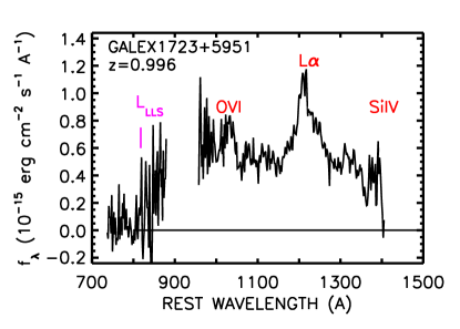

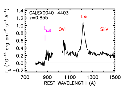
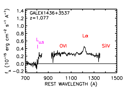
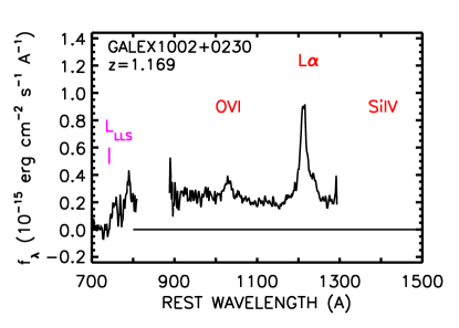
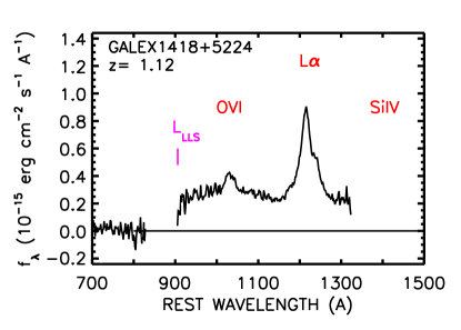
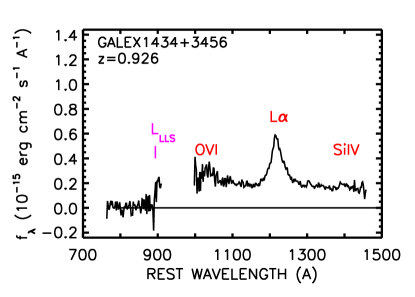
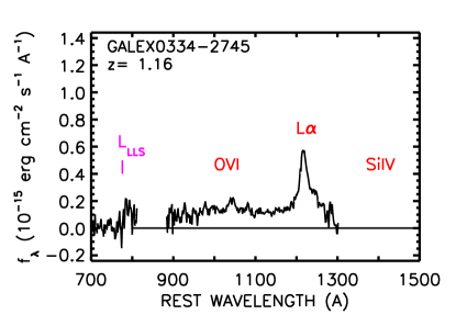
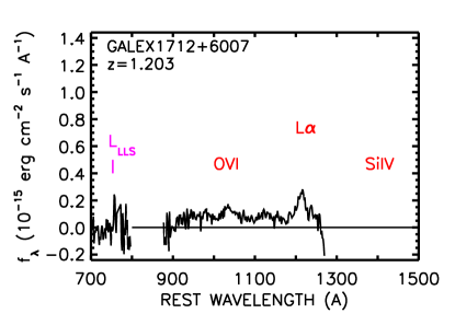
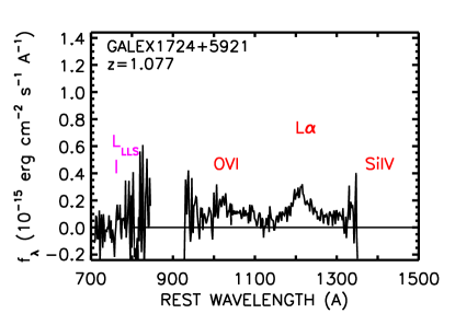
We inspected all of the GALEX spectra for these objects and picked out those with strong LLS (). To do this we fitted a power law continuum to the spectrum above and then found the first location at which the spectrum dropped by more than a factor of 2.7 and did not subsequently recover at shorter wavelengths. The GALEX spectra in which we detected such a strong LLS are shown in Figure 4 (see also Appendix), where we order the sample by the red continuum flux. An important point to note is that the GALEX spectra consist of two wavelength segments: one corresponding to the FUV grism ( Å) and one to the NUV grism ( Å). We can still select LLS in the range since the flux break across the gap is easily seen; consequently, the search pathlength is the redshift range including the gap. In the case where a LLS did fall in the gap, we would not be able to make a precise measurement of the break redshift and we would have to address the redshift uncertainty in the analysis. In fact we do not find any LLS in our sample whose redshift lies in the gap. LLS systems were found in 9 of the 50 quasars at redshifts above the limit where we could have detected such a system, though one system (in GALEX 1418+5223) lies close to this region and we consider the changes in the results that would be produced if it lies at a lower redshift. The LLS in GALEX 1724+5921 is somewhat uncertain because of the noisy spectrum. We examine the reduction in the number density which would be produced by removing it in the analysis.
| Redshift bin | # QSO | # LLS | Error | ||
|---|---|---|---|---|---|
| (0.36,1.1)a | 51 | 11 | 0.63 | 0.19 | 0.64 |
| (0.58,1.25)b | 49 | 7 | 0.30 | 0.12 | 0.82 |
| (0.36,1.25)c | 100 | 18 | 0.44 | 0.10 | 0.72 |
| (2.4,2.9) | 77 | 29 | 1.84 | 0.33 | 2.74 |
| (2.9,3.8) | 106 | 52 | 2.43 | 0.33 | 3.20 |
| (3.8,4.2) | 52 | 31 | 3.77 | 0.64 | 4.04 |
| (4.2,5.0) | 61 | 33 | 4.04 | 0.70 | 4.39 |
| (5.0,6.0) | 8 | 6 | 8.91 | 3.49 | 5.69 |
3. Lyman Limit Systems
We first computed the number density of LLS per unit redshift path d, which we write as . As is conventional, we excluded LLS lying within of the quasar and computed the redshift path accordingly. The data can be analysed assuming a constant density of sources in a redshift interval or as a fit to an assumed redshift evolution over the entire redshift interval. To determine and its error in each redshift interval we used the maximum likelihood fit (MLF) in the form given by SSB. The corresponding results are shown in Figure 5. For the higher redshift interval we have shown only the full samples (the present data and all previous data taken from the compilation of P03). However, for we have shown the results obtained separately from the present GALEX sample (blue diamond) and the older SL95 sample (red triangle) as well as that for the combined sample. We have chosen to show the independent values since it is possible that the difference could reflect systematic selection effects in the archival UV observed quasar samples analysed by SL95 which might result in an upward bias in the LLS density. However, the SL95 and GALEX samples are consistent within the statistical uncertainties and we shall use the combined value in the following text. The present data roughly doubles the low redshift sample and provides a corresponding reduction in the error over the previous SL95 result (Table 3). The values of in each redshift interval are summarized in Table 3, where we give the redshift bin, the number of QSOs used, the number of LLS detected, the value of and its error, and the average redshift of the LLS. For the combined sample, we find a value of . If the LLS in GALEX 1724+5921 is eliminated the values in the interval would reduce to , while if the redshift of the LLS in GALEX 1418+5223 is lowered to 0.97, the value is unchanged at the quoted level of significance. We have eliminated the LLS in GALEX 1724+5921 in the subsequent analysis and the numbers in Table 3 correspond to the sample excluding this quasar.
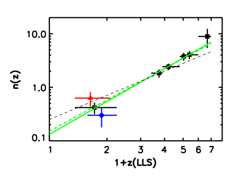
We also examined the effects of the estimated redshift and optical depth errors derived from the simulation and discussed in the previous section and shown in Figure 3. For – 5, reducing the LLS redshift by the offset for the case would reduce the measured from to 3.77 and at – 6, reducing the LLS redshift by would change from to 7.03. The effect is smaller for higher optical depth systems and the systematic changes are smaller than the statistical uncertainty. The 0.3 scatter in optical depth introduces an Eddington bias since there are more low- systems to scatter up than scatter down. However, this effect is also very small, a few percent in , compared with the statistical error.
In analysing the redshift evolution of the LLS it is usual to parameterize the evolution in as
| (1) |
where is the value of at , and to estimate the parameters using a maximum-likelihood fit to the full data set in a given redshift interval. The motivation for this form lies in the historical description, based on assuming that LLS lie in galactic haloes, but it is also a simple parameterization which provides a reasonable choice of form fitting for the sample and is useful for comparing with previously derived results. However, the use of results in a strong coupling between this parameter and , reflecting the lever arm in the power law. This may be avoided, and the display of the parameter fit simplified, by normalizing nearer to the center of the redshift range and we use the form
| (2) |
where is the value of at , to show the error contours on the parameters.
We calculated the log-likelihood function
| (3) |
where the notation follows that of Péroux (2001) and is the number of LLS and is the number of quasars, and used this to estimate and and their errors in the redshift intervals and . The results are summarized in Table 4, where we also list the parameters and fitting ranges of previous fits from the literature.
| Samplea | Redshift range | QSO | LLSb | |||
|---|---|---|---|---|---|---|
| This paper | 1.5 – 6 | 216 | 157 | 0.13 | ||
| 0.0 – 6 | 315 | 175 | 0.15 | |||
| Ref. (1) | 0.40 – 4.93 | 148 | 84 | |||
| Ref. (2) | 0.32 – 4.11 | 169 | 80 | |||
| Ref. (3) | 0.40 – 4.69 | 90 | 48 | |||
| Ref. (4) | 0.67 – 3.58 | 90 | 54 | 0.76 | ||
| Ref. (5) | 3.3 – 4.4 | 469 | 192 |
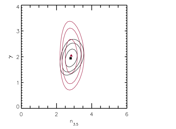
The fits are shown in Figure 5 as the solid () and dashed () green lines, compared with the redshift evolution of the density of LLS in the complete quasar sample (filled black squares) in suitable redshift bins. In contrast with previous results, and primarily as a consequence of the new low-redshift value, the fits over the two redshift ranges are practically indistinguishable and give consistent values for and , as is seen in Figure 6, which plots the 1, 2, and error contours. A single parameterizaton (, ) fits well over the entire redshift range, . The evolution inferred with this data set is generally steeper than previously measured (see Table 4), except for the result of Péroux (2001). In particular, the evolution is steeper than that measured by SL95 for , (the black dashed line in Figure 5), as a result of the improved low-redshift determination from the large combined sample.
4. Damped Lyman Alpha Systems
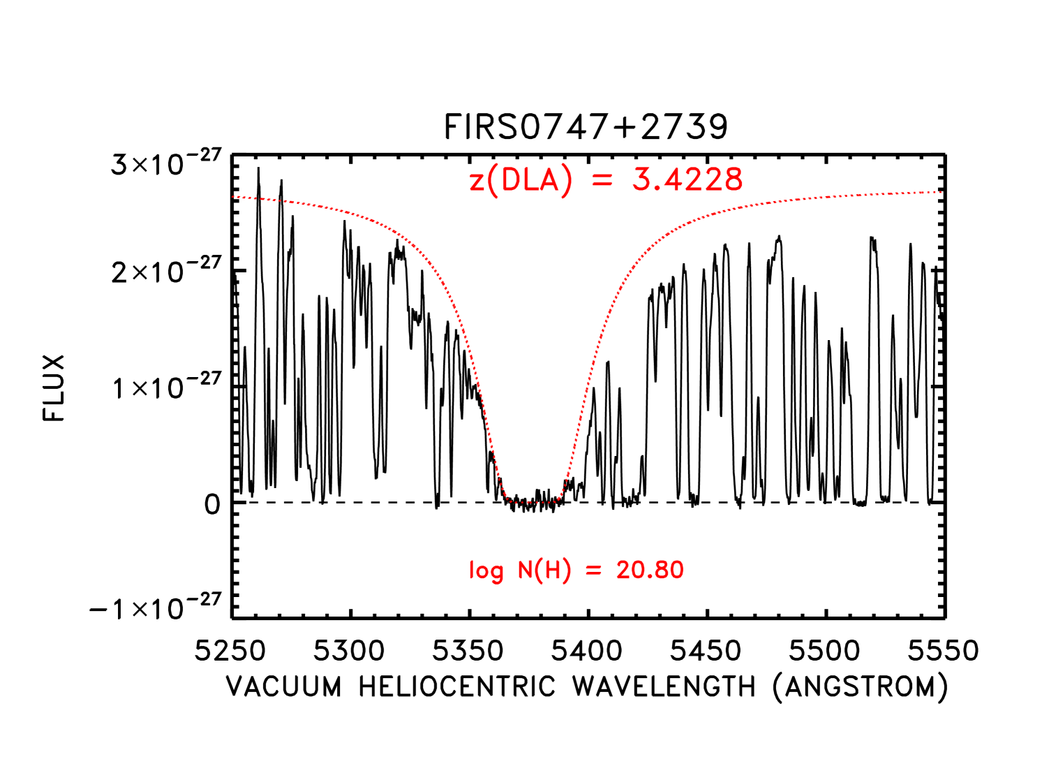
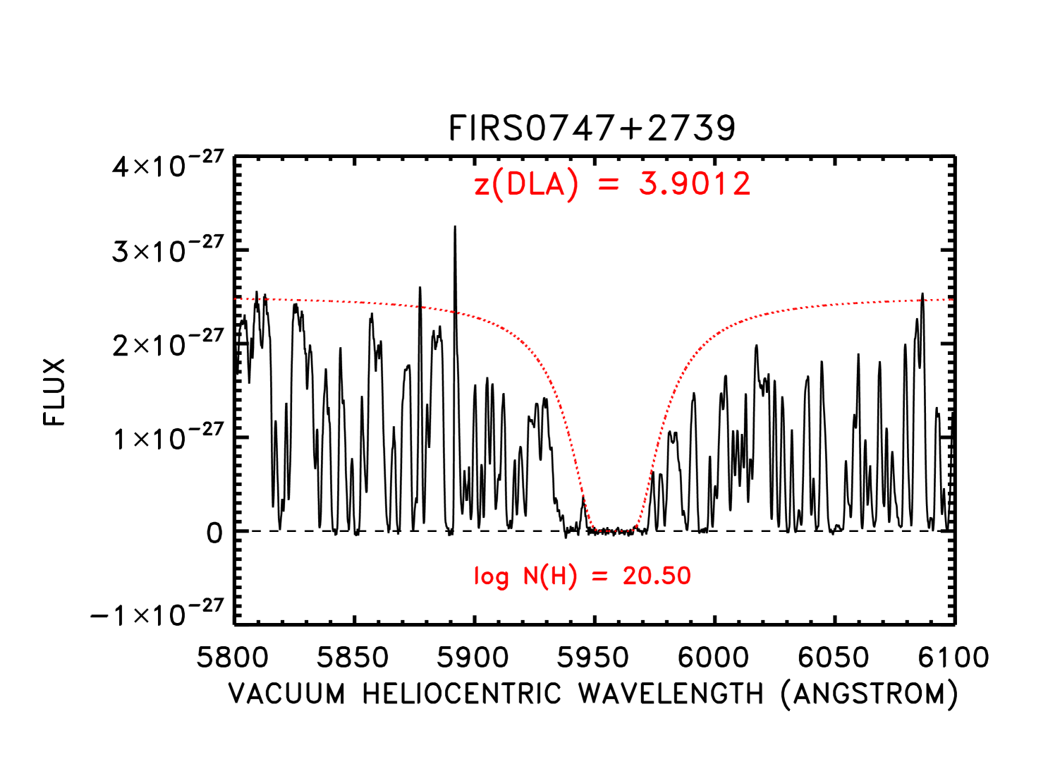
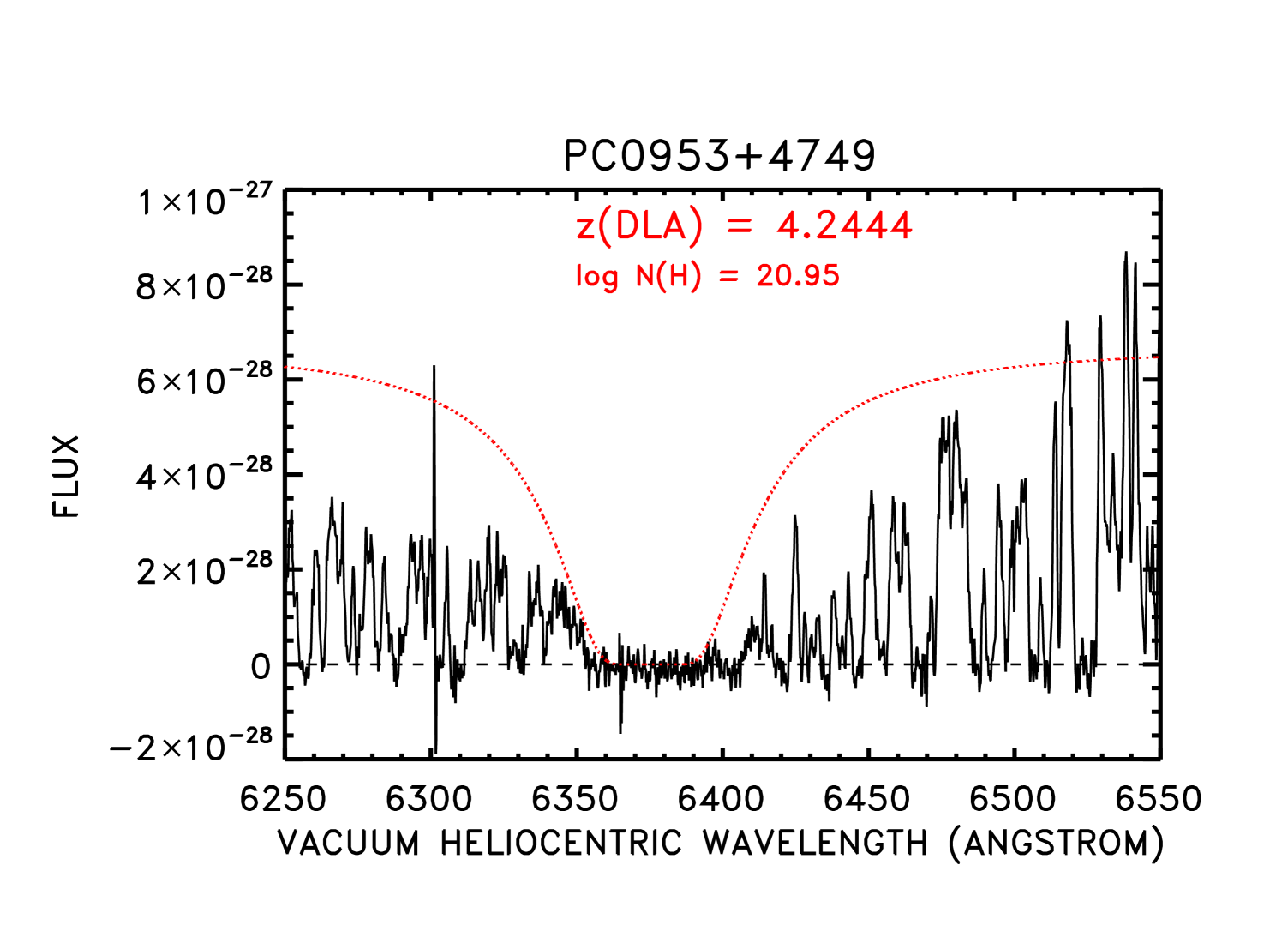
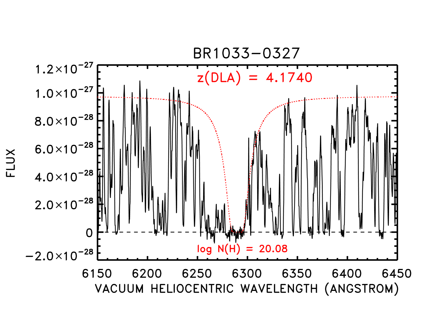
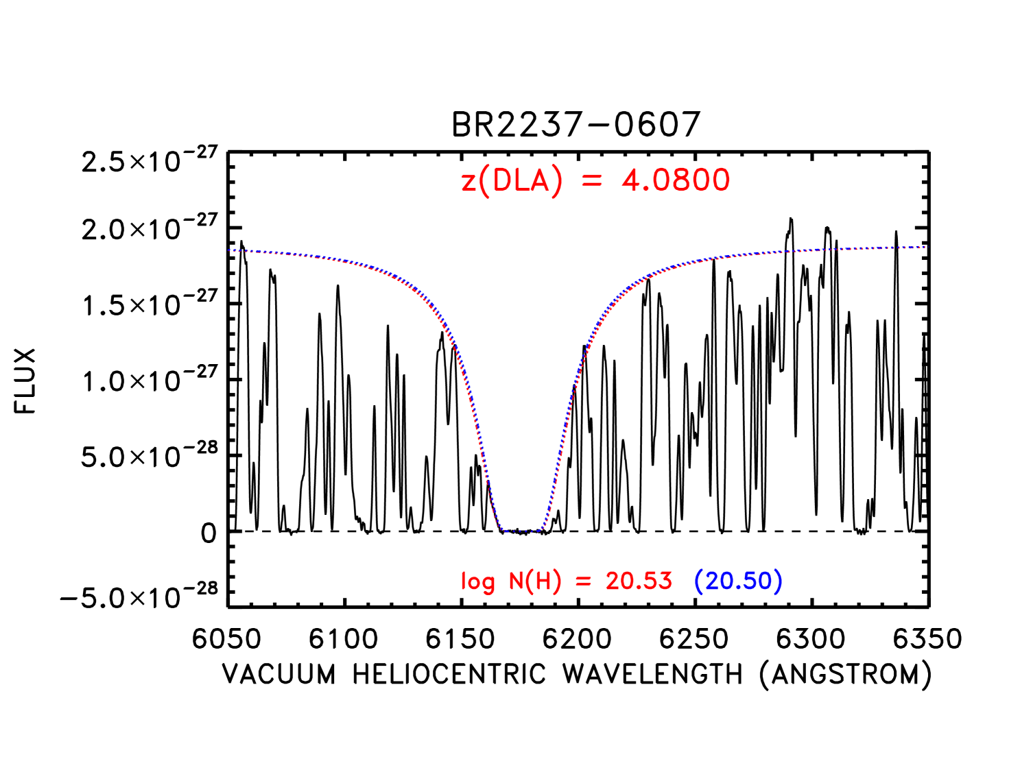
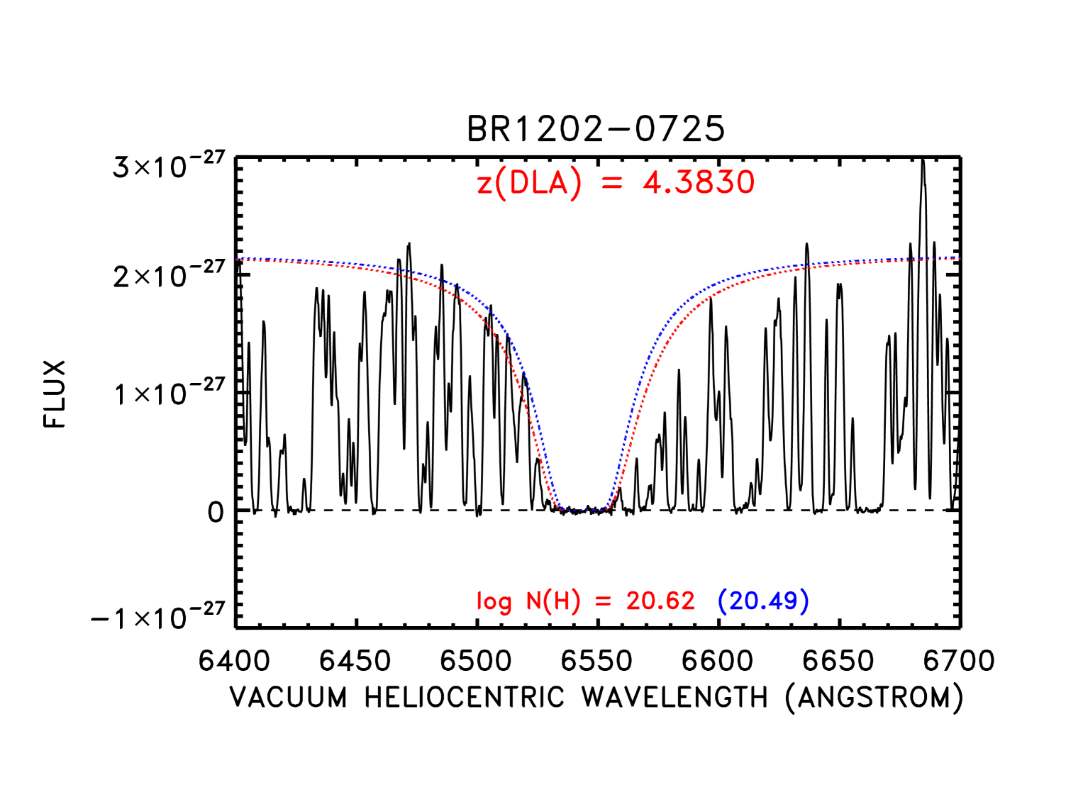
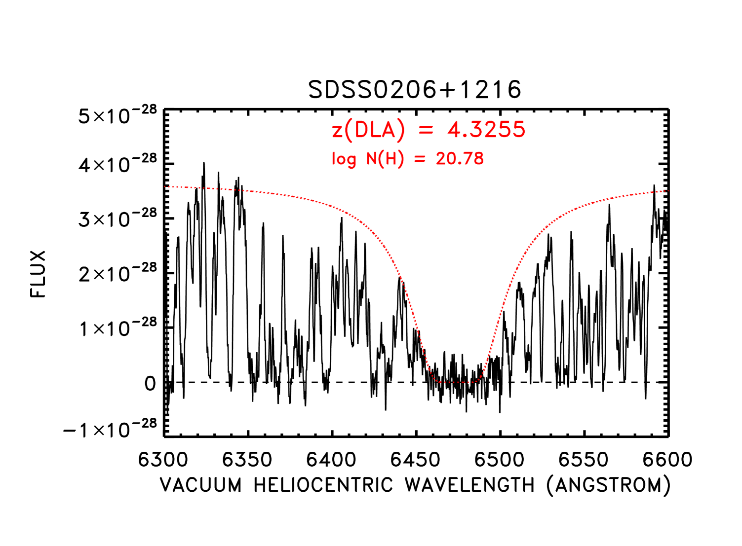
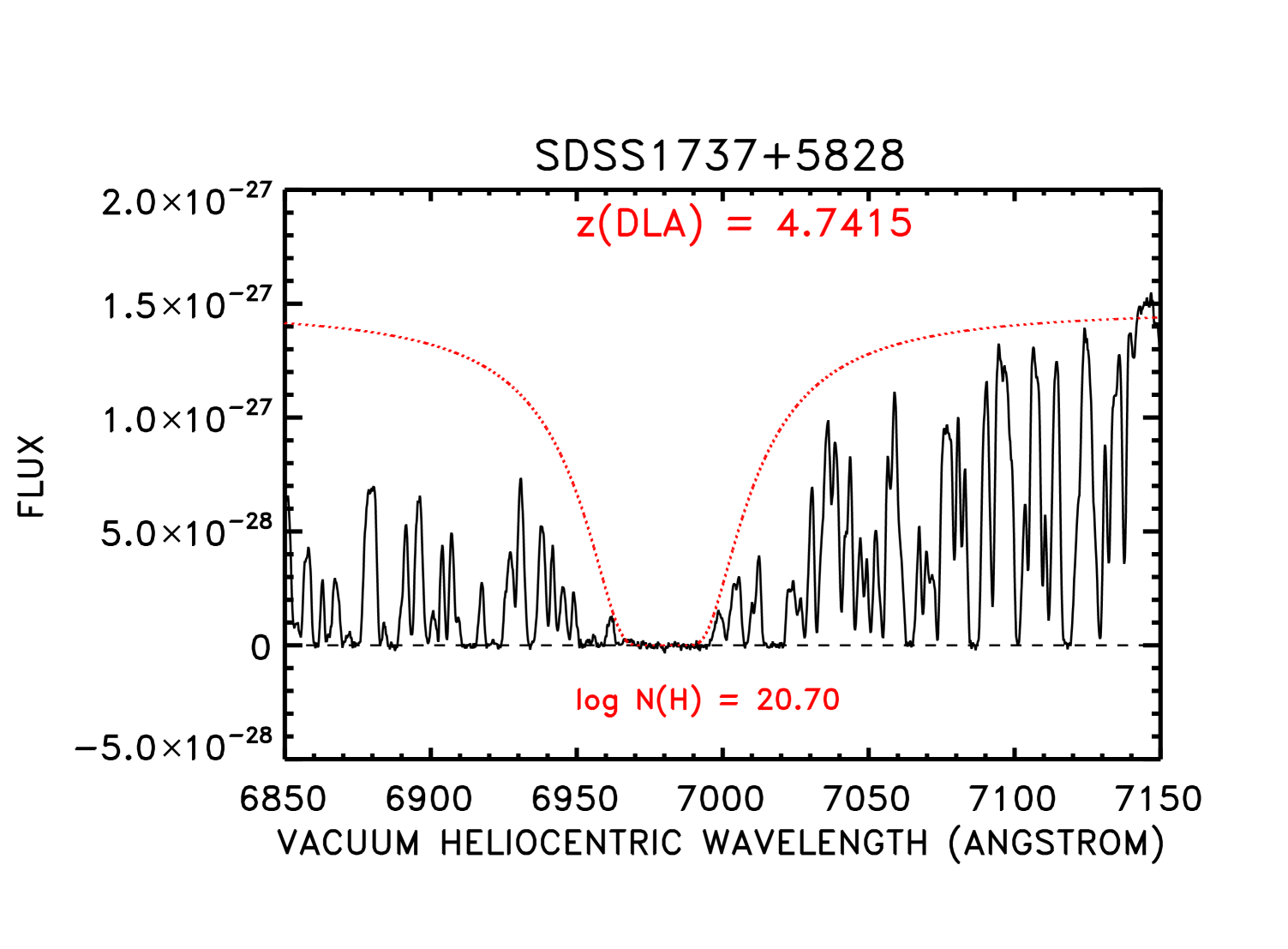
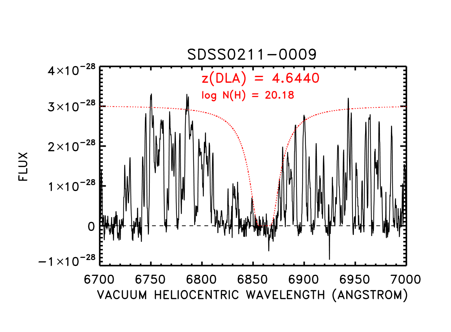
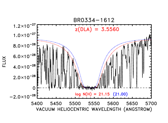
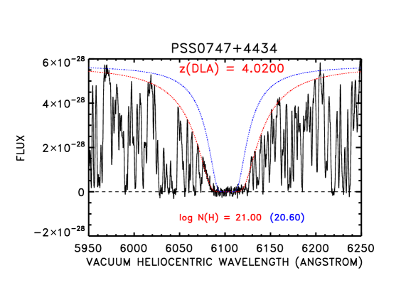
We searched the spectra for absorption lines with damping wings and found a total of 17 DLAs () and sub-DLAs () within our quasar sample, 14 DLAs and 3 subDLAs. We believe the sample is complete to the level . However, in the highest redshift quasars the lower column density systems are hard to measure and we have not attempted to extend the measurements below . DLAs in general become too hard to measure beyond because of the thickness of the forest. We measured for these systems by fitting to the damping wings (Figure 7 and Appendix), and column 8 of Table 1 compares our measured values of with previous measurements from Prochaska et al. (2007) and P03. Fourteen of the systems have existing measurements. All of the DLAs in the present sample are shown in Figure 7 together with the damped fits (red solid lines). Nine of the DLAs overlap with DLAs in the P03 sample and the P03 fits are shown with blue dotted lines in Figure 7. One DLA in the P03 sample is classified as a sub-DLA here (the system in PSS0741+4434), and one DLA in the P03 sample (the system in SDSS0338+002) is not confirmed. However, in general the measured column densities agree well with previous measurements. The present sample substantially increases the path length above . We summarize the present results combined with quasars from P03 and Guimarães et al. (2009) in Table 5. We have used these combined samples to compute the redshift evolution of DLAs out to to compare with that of the LLS.
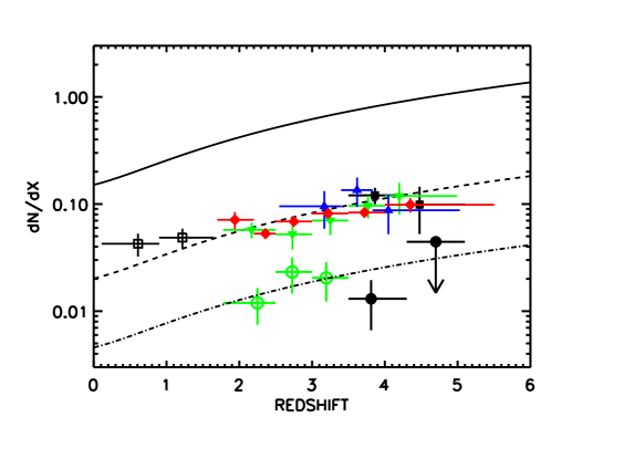
In Figure 8 we compare the redshift evolution of the DLAs with those of the LLS. The black line shows the maximum likelihood fit to the evolution of in the LLS over the range , where d is defined as
| (4) |
and d is the number of LLS in the interval d. The black squares show the observed number of DLAs with in the redshift intervals [3.5,4.3], and [4.3,5.1], computed from the present data set combined with preceding measurements. The error bars are based on the Poisson errors corresponding to the number of systems in the bin (Gehrels 1986). We have also computed the errors using a jackknife estimation. These agree well for bins with higher numbers of systems but underestimate the error in bins with only a small number of DLAs. We also show lower redshift DLA number density measurements from the literature (Prochaska et al. 2005, Péroux et al. 2005, Rao et al. 2006 and Guimarães et al. 2009.) The black circles show the distribution for the systems with the P03 results shown with green open circles.
If the neutral hydrogen column density distribution function is invariant with redshift the redshift evolution of the LLS and the DLAs would have the same form in Figure 8. This appears to be the case for the systems where a simple scaling down of the LLS numbers by a factor of 7.5 replicates the evolution of the DLAs, at least for . The situation is less clear for the higher column density () DLAs. At low redshifts () the LLS can be scaled down by a factor of 33 to match the high column density DLAs but the errors at high redshift could permit a substantial deviation from this form. We adopt a single power-law fit, , to the column density distribution as a function of redshift between the LLS () and DLA ( and 21.0) column densities. For the individual points are consistent with a single index of for , whereas an index of is required for . The steeper index over the wider column density range is a consequence of the well known turnover in the column density distribution function at high column density (e.g. Petitjean et al. 1993; Storrie-Lombardi & Wolfe 2000; Prochaska et al. 2005; O’Meara et al. 2007; Guimarães et al. 2009).
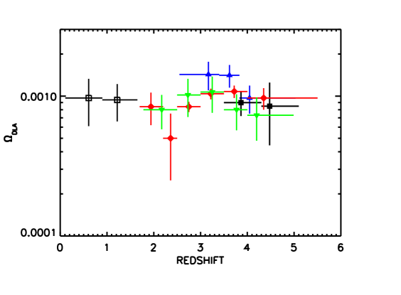
Finally, we have computed for the combined sample for and and compare these values with results from the literature in Figure 9 ( here includes both hydrogen and helium). The present data (black squares and error bars) show no evolution in to (see also Prochaska et al. 2005; Péroux et al. 2005; Noterdaeme et al. 2009; Guimarães et al. 2009). This remains true if we expand the sample to include the subDLAs, which raises by about 30% in the highest redshift bin. The evolution is consistent with a constant over the observed redshift range.
| Quasar | Sourcea | Otherb | ||||
|---|---|---|---|---|---|---|
| PSS1140+6205 | 4.500 | 3.113 | 0.000 | 0.00 | 1 | |
| PSS0808+5215 | 4.510 | 3.181 | 3.114 | 20.60 | 1 | |
| BR10330327 | 4.510 | 2.888 | 4.174 | 20.08 | 0 | |
| PSS1723+2243 | 4.515 | 3.062 | 3.697 | 20.35 | 1 | |
| PSS1715+3809 | 4.520 | 3.004 | 3.341 | 21.05 | 1 | |
| BR00191522 | 4.528 | 2.970 | 3.437 | 20.92 | 2 | |
| PSS0134+3307 | 4.536 | 2.976 | 3.760 | 20.60 | 1 | P 20.6 |
| BR22370607 | 4.550 | 2.941 | 4.080 | 20.53 | 0 | P 20.50 |
| PSS1347+4956 | 4.565 | 2.963 | 0.000 | 0.00 | 0 | |
| BR03533820 | 4.580 | 3.022 | 0.000 | 0.00 | 0 | |
| BR12020725 | 4.610 | 3.112 | 4.383 | 20.62 | 0 | P 20.49 |
| SDSS0210001 | 4.700 | 3.177 | 0.000 | 0.00 | 1 | P 20.5 (3.420)∗ |
| BRJ03074945 | 4.728 | 3.138 | 4.460 | 20.80 | 2 | |
| SDSS2200+001 | 4.780 | 3.214 | 0.000 | 0.00 | 0 | |
| SDSS 0206+121 | 4.810 | 3.007 | 4.326 | 20.78 | 0 | |
| SDSS0941+594 | 4.820 | 3.322 | 0.000 | 0.00 | 1 | |
| PSS1247+3406 | 4.897 | 3.314 | 0.000 | 0.00 | 1 | |
| SDSS0211000 | 4.900 | 3.255 | 4.644 | 20.18 | 0 | |
| SDSS1737+582 | 4.850 | 3.309 | 4.741 | 20.70 | 0 | PW 20.65 |
| SDSS0338+002 | 5.010 | 3.480 | 0.000 | 0.00 | 0 | P 20.4 (4.060)∗ |
| SDSS1204002 | 5.070 | 3.437 | 0.000 | 0.00 | 0 | |
| SDSS0756+410 | 5.090 | 3.551 | 4.360 | 20.15 | 1 |
5. Discussion
The density evolution of the LLS is most closely related to the attenuation length of ionizing photons in the intergalactic medium since it is systems with column densities near the value of the LLS that dominate the neutral hydrogen opacity. Thus the conversion of , the source function of ionizing photons, to , the ionization rate in the intergalactic medium, can be determined if we know the evolution of the LLS and the shape of the column density distribiution in the neighborhood of the LLS column density.
Following the fundamental work of Madau, Haardt and Rees (1999; MHR), there have been a number of revisits to the problem, updating the calculation using recent values of the evolution parameters and the column density shape. The most recent version is given by Faucher-Giguère et al. (2008). At these calculations are enormously simplified by the short mean free path of the photons which means the calculation is essentially local (MHR). In this limit, if we can approximate the column density distribution function in the neighborhood of the LLS column density as , the mean free path is simply related to the LLS system density as
| (5) |
or
| (6) |
where is the optical depth at the Lyman edge, is the optical depth above which is measured (here ) and is the frequency of the Lyman continuum edge (see for example the equations in Miralda-Escudé (2003) or Choudhury (2009), and note that in this equation is the gamma function and not the ionization rate). MHR adopted redshift-invariant values of and to calculate the values, basing these parameters on the work of Petitjean et al. (1993), Hu et al. (1995), and Kim et al. (1997) for the index. Faucher-Giguère et al. (2008) updated the parameter to using the results of Misawa et al. (2007), used Stengler-Larrea’s fit to the LLS population, and again assumed a redshift-invariant set of parameters.
The present work supports the assumption of redshift invariance, and our power law index fit of to the cumulative distribution between the LLS and the DLA column densities is not substantially different (in the differential form of ) from the Misawa et al. (2007) value adopted by Faucher-Giguère. However, the present data implies a higher value of the LLS density at than was adopted by Faucher-Giguère, with a corresponding decrease in the mean free path since, as was already known from the work of P03, the SL95 fit to the high redshift LLS is low because their sample did not extend to higher redshifts. Combining the evolutionary form of the LLS with equation (6), and using the high redshift approximation, , gives
| (7) |
where we have used the normalization at which places the errors primarily in the exponent (see Figure 6). For , the maximum likelihood fit for gives
| (8) |
For , the normalization becomes 37 Mpc and for , 61 Mpc.
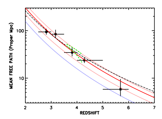
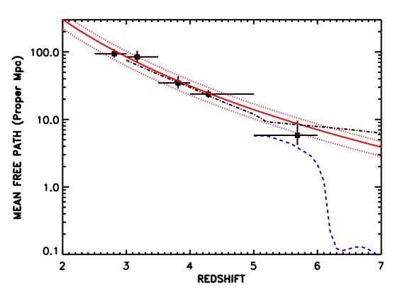
We show the mean free path of equation (7), and also that computed from the measured at that redshift, in Figure 10, where we compare with the mean values computed by MHR and Faucher-Giguère et al. (2008) and with the mfp determination of Prochaska et al. (2009a) in the range . Note that the errors shown are formal statistical errors only and there may be additional systematic errors. Rescaled to the present cosmology, the MHR value is which, while very similar in shape, is about a factor of two lower than the present results. The mean free path has a steeper slope than that of Faucher-Giguère and is reduced by a factor of 1.2 at , increasing the emissivity required to ionize the IGM by the same factor. This increases the well-known discrepancy between the required and known sources of ionization at these high redshifts relative to the results of that paper.
Fan et al. (2006) have made an estimate of the mfp based on the measured transmission and an assumed log normal density distribution function, following Miralda-Escudé, Haehhnelt & Rees (2000). This procedure is very uncertain at the high redshifts where the transmission is dominated by the extreme underdense tail of the distribution function, which is poorly described by the log normal function (Becker et al. 2007). Perhaps not surpisingly, given this and other major uncertainties in the interpretation, the Fan et al. (2006) estimates are steeper in shape and about a factor of 2.5 – 4 lower in normalization than the present measurements in the interval .
The steep drop in the mfp with redshift to , if extrapolated to higher redshift, predicts a very small proper length value of around 5 Mpc at . If this is smaller than the size of the HII bubbles at the overlap epoch there could be important consequences for the evolution of the ionization rate (e.g. Furlanetto and Mesinger 2009).
However, it is probable that as we move to earlier periods the evolution of the geometry and ionization rates will combine to modify the evolution of the LLS, and simple extrapolations to higher redshifts might not be justified despite the smooth evolution from . Full numerical simulations, capable of the resolution required to describe the Lyman limit systems, are still extremely challenging and subject to many uncertainties. In Figure 10 we compare the present observations with the simulation of Kohler & Gnedin (2007) and Gnedin & Fan (2006). These models are not a particularly good description of the lower redshift mfp or , presumably because of uncertainties in the evolution of the intergalactic ionization parameter. However, they emphasize that the mfp could evolve smoothly to and then change rapidly at higher redshifts. In this case the models correspond to reionization just above and the mean free path drops rapidly above this redshift.
However, even the sign of the evolution in the mean free path is poorly determined at high redshift. Choudhury & Ferrara (2005, 2006) and Choudhury (2009) have computed semi-analytic models based on the formalism of Miralda-Escudé (2003) with ionization histories chosen to match the high redshift constraints. These models provide a very good match to the LLS density. However, as can be seen in Figure 10, they predict that the mfp flattens above and the drops. In these models the bulk of the IGM volume is still ionized up to and the change in the mfp corresponds to the transition away from popIII ionization at redshifts .
We conclude that it is probably wise not to extrapolate the mfp beyond the measured range. However, the shape and normalization of the mfp evolution at may still provide useful tests of the higher redshift evolution since any model must satisfy the boundary condition.
References
- (1)
- (2) Bechtold, J., Dobrzycki, A., Wilden, B., Morita, M., Scott, J., Dobrzycka, D., Tran, K.-V., & Aldcroft, T. L. 2002, ApJS, 140, 143
- (3) Becker, G. D., Rauch, M., & Sargent, W. L. W. 2007, ApJ, 662, 72
- (4) Choudhury, T. R. 2009, arXiv:0904.4596
- (5) Choudhury, T. R. & Ferrara, A. 2005, MNRAS 361, 577
- (6) Choudhury, T. R. & Ferrara, A. 2006, MNRAS 371, L55
- (7) Cowie, L. L., Barger, A. J., & Hu, E. M. 2010, ApJ 711, 928
- (8) Fan, X., et al. 2006, AJ, 132, 117
- (9) Faucher-Giguère, C.-A., Lidz, A., Hernquist, L., & Zaldarriaga, M. 2008, ApJ, 688, 85
- (10) Furlanetto, S. R.. & Mesinger, A. 2009, MNRAS, 394, 1667
- (11) Gehrels, N. 1986, ApJ, 303, 336
- (12) Gnedin, N. Y., & Fan, X. 2006, ApJ, 648, 1
- (13) Guimarães, R. et al. 2009, A&A, 508, 133.
- (14) Hu, E. M., Kim, T.-S., Cowie, L. L., Songaila, A., & Rauch, M. 1995, AJ 110, 1526
- (15) Kim, T.-S., Hu, E. M., Cowie, L. L., & Songaila, A. 1997, AJ, 114, 1
- (16) Kohler, K., & Gnedin, N. Y. 2007, ApJ, 655, 685
- (17) Lanzetta, K., 1991, ApJ, 375, 1
- (18) Lanzetta, K., Wolfe, A. & Turnshek, D., 1995, ApJ, 440, 435
- (19) Madau, P., Haardt, F. & Rees, M. J. 1999, ApJ, 514, 648 (MHR)
- (20) Miralda-Escudé, J. 2003, ApJ, 597, 66
- (21) Miralda-Escudé, J., Haehnelt, M., & Rees, M. J. 2000, ApJ, 530 1
- (22) Misawa, T., Tytler, D., Iye, M., Kirkman, D., Suzuki, N., Lubin, D. & Kashikawa, N. 2007, AJ, 134, 1634
- (23) Morrissey, P., et al. 2007, ApJS, 173, 682
- (24) Noterdaeme,P., Petitjean, P., Ledoux, C., & Srianand, R. 2009, A&A, 505, 1087
- (25) O’Meara, J. M., Prochaska, J. X., Burles, S., Prochter, G., Bernstein, R. A., & Burgess, K. M. 2007, ApJ 656, 666
- (26) Péroux, C. 2001, Ph. D. Thesis, Cambridge University
- (27) Péroux, C., Dessauges-Zavadsky, M., D’Odorico, S., Sun Kim, T., & McMahon, R. G. 2005, MNRAS, 363, 479.
- (28) Péroux, C., McMahon, R. G., Storri-Lombardi, L. J., & Irwin, M. J. 2003, MNRAS, 346, 1103 [P03]
- (29) Petitjean, P., Webb, J., Rauch. M., Carswell, R., & Lanzetta, K., 1993, MNRAS, 262, 499
- (30) Prochaska, J. X., Herbert-Fort, S., & Wolfe, A. M. 2005, ApJ, 635, 123.
- (31) Prochaska, J. X., O’Meara, J. M., & Worseck, G. 2010, ApJ, 718, 392.
- (32) Prochaska, J. X., Wolfe, A. M., Howk, J. C., Gawiser, E., Burles, S. M., & Cooke, J. 2007, ApJS, 171, 29.
- (33) Prochaska, J. X., Worseck, G., & O’Meara, J. M. 2009, ApJ, 705, L113.
- (34) Rao, S. M., Turnsheck, D. A., & Nestor, D. B. 2006, ApJ, 636, 610.
- (35) Sargent, W. L. W., Steidel, C. C., & Boksenberg, A. 1989, ApJS, 69, 703 [SSB]
- (36) Stengler-Larrea, E. A., et al. 1995, ApJ, 444, 64 [SL95]
- (37) Storrie-Lombardi, L., McMahon, R., Irwin, M. & Hazard, C., 1994, ApJ, 427, L13
- (38) Storrie-Lombardi, L. & Wolfe, A. M. 2000, ApJ, 543, 552
- (39) Tytler, D., 1982, Nature, 298, 427


