\catchline

Ellipticity of Structures in CMB Sky Maps

Ralf Aurich    Holger S. Janzer    Sven Lustig Institut für Theoretische Physik, Universität Ulm,
Albert-Einstein-Allee 11, D-89069 Ulm, Germany
   Frank Steiner Université Lyon 1, Centre de Recherche Astrophysique de Lyon
CNRS UMR 5574, 9 avenue Charles André, F-69230 Saint-Genis-Laval, France
Abstract

We study the ellipticity of contour lines in the sky maps of the cosmic microwave background (CMB) as well as other measures of elongation. The sensitivity of the elongation on the resolution of the CMB maps which depends on the pixelization and the beam profile of the detector, is investigated. It is shown that the current experimental accuracy does not allow to discriminate between cosmological models which differ in curvature by ΔΩtot=0.05ΔsubscriptΩtot0.05\Delta\Omega_{\hbox{\scriptsize tot}}=0.05. Analytical expressions are given for the case that the statistical properties of the CMB are those of two-dimensional Gaussian random fields.

keywords:
cosmology, cosmic microwave background, statistic, Gaussian random fields

1 Introduction

The cosmic microwave background (CMB) gives a wealth of information about the Universe. The usual statistical analysis comprises the angular auto-correlation function C(ϑ)𝐶italic-ϑC(\vartheta) as well as the angular power spectrum δTl2𝛿superscriptsubscript𝑇𝑙2\delta T_{l}^{2}, which lead to an improved determination of the cosmological parameters. Besides these statistics there are topological/geometrical descriptors of the CMB such as the number densities of maxima and minima, the ellipticities of the peaks, and peak correlation properties. Under the assumption that the CMB has the statistical properties of two-dimensional homogeneous and isotropic Gaussian random fields, the theoretical predictions are derived in Ref. \refciteBond_Efstathiou_1987.

This paper deals with the structure of the contour lines of a given temperature level δT𝛿𝑇\delta T in the CMB maps. In the vicinity of extrema these contour lines can be approximated by ellipses having the ellipticity E𝐸E

E:=ab,E 1,E\;:=\;\frac{a}{b}\hskip 10.0pt,\hskip 10.0ptE\;\geq\;1\hskip 10.0pt, (1)

where ab𝑎𝑏a\geq b denote the major and minor semi-axes of the ellipses which best match the contour line around a given peak. The interesting question is how the ellipticities are distributed for a given map in dependence on the temperature level δT𝛿𝑇\delta T. This provides a further test[2, 3] of Gaussianity by comparing the ellipticities with the corresponding results of two-dimensional Gaussian random fields[1]. In Refs. \refciteBarreiro_Sanz_Martinez-Gonzalez_Cayon_Silk_1997,Barreiro_Martinez-Gonzalez_Sanz_2001,Monteserin_Barreiro_Sanz_Martinez-Gonzalez_2005 it is shown, however, that there are better geometrical estimators as tests of Gaussianity than the ellipticity like the Gaussian curvature. Therefore, the main motivation for this paper is to study the discrepancy of the ellipticity between the observations and simulations of the CMB as reported in Refs. \refciteGurzadyan_Torres_1997,Gurzadyan_et_al_2003a,Gurzadyan_et_al_2003b,Gurzadyan_et_al_2004,Gurzadyan_et_al_2005,Gurzadya_et_al_2007. In these papers an excess in the ellipticity E=2.22.7𝐸2.22.7E=2.2\dots 2.7 is found compared to standard ΛΛ\LambdaCDM models having E𝐸E around 1.65. Due to noise and the foreground uncertainties it is difficult to obtain the ellipticity from the measured CMB radiation. The ellipticity was determined from the COBE-DMR map[7] and from the BOOMERanG map[8, 9]. These results are confirmed by the analysis of the WMAP 1yr data[10, 11] and the 3yr data[12]. Furthermore, a strong dependence of the ellipticity on the curvature of the Universe is claimed and, with respect to the excess ellipticity, this is interpreted as a hint towards a hyperbolic Universe. In Ref. \refciteBarreiro_Sanz_Martinez-Gonzalez_Cayon_Silk_1997 there is no such ellipticity-curvature correlation found by studying low ΩΩ\Omega and flat universes based on CDM models. Thus there remains the question whether the excess ellipticity is real and how such an excess, if present, has to be interpreted.

2 CMB Sky Maps

2.1 Cosmological models

The standard ΛΛ\LambdaCDM model of cosmology is given by a certain set of cosmological parameters. The curvature of the universe is determined by the value of the total energy density ΩtotsubscriptΩtot\Omega_{\hbox{\scriptsize tot}} at the present epoch which is the sum

Ωtot=ΩΛ+Ωcdm+Ωb+ΩrsubscriptΩtotsubscriptΩΛsubscriptΩcdmsubscriptΩbsubscriptΩr\Omega_{\hbox{\scriptsize tot}}\;=\;\Omega_{\Lambda}+\Omega_{\hbox{\scriptsize cdm}}+\Omega_{\hbox{\scriptsize b}}+\Omega_{\hbox{\scriptsize r}} (2)

of the energy density ΩΛsubscriptΩΛ\Omega_{\Lambda} of dark energy, ΩcdmsubscriptΩcdm\Omega_{\hbox{\scriptsize cdm}} of cold dark matter, ΩbsubscriptΩb\Omega_{\hbox{\scriptsize b}} of baryonic matter and ΩrsubscriptΩr\Omega_{\hbox{\scriptsize r}} of radiation. A value Ωtot>1subscriptΩtot1\Omega_{\hbox{\scriptsize tot}}>1, =1absent1=1 or <1absent1<1 reveals a spherical, flat or hyperbolic universe, respectively. The concordance ΛΛ\LambdaCDM model[13, 14] leads to a flat universe where the angular power spectrum δTl2=l(l+1)Cl/(2π)𝛿superscriptsubscript𝑇𝑙2𝑙𝑙1subscript𝐶𝑙2𝜋\delta T_{l}^{2}=l(l+1)C_{l}/(2\pi) has the first acoustic peak at l220similar-to-or-equals𝑙220l\simeq 220. The following analysis investigates the dependence of the ellipticity on the curvature of the universe. To that aim only the amount of dark energy ΩΛsubscriptΩΛ\Omega_{\Lambda} is varied, all other cosmological parameters are those of the ΛΛ\LambdaCDM concordance model.

In addition to the infinite volume ΛΛ\LambdaCDM concordance model, a model with a cubic topology[15, 16] is also studied which has a finite volume and is statistically anisotropic. This model thus violates some conditions required for the following analytical expressions as outlined in the Appendix. This model serves as a test whether an anisotropic non-trivial topology can be discerned by an elongation measure. The sky maps are simulated for the cubic topology using the same cosmological parameters as for the infinite concordance model. The side length L𝐿L of this toroidal topology is chosen as L=3.86LH𝐿3.86subscript𝐿𝐻L=3.86\,L_{H} where LHsubscript𝐿𝐻L_{H} is the Hubble length. For this length L𝐿L a better agreement with the correlations observed in the CMB sky is found[15, 16, 17] than for the ΛΛ\LambdaCDM concordance model. The eigenmodes belonging to the first 50 000 eigenvalues for the cubic topology are used for the simulation, i. e. a total of 61 556 892 eigenmodes. Furthermore, the eigenmodes are expanded in the spherical basis up to lmax=1000subscript𝑙max1000l_{\hbox{\scriptsize max}}=1000 yielding sky maps with structures beyond the third acoustic peak where the Silk damping already smoothes a further fine-structure. In this way CMB sky simulations are obtained for which resolution effects can be studied.

For a given cosmological model, i. e. a given set of cosmological parameters, one can calculate the multipole spectrum

Cl:=12l+1m=ll|alm|2,assignsubscript𝐶𝑙delimited-⟨⟩12𝑙1superscriptsubscript𝑚𝑙𝑙superscriptsubscript𝑎𝑙𝑚2C_{l}\;:=\;\left\langle\frac{1}{2l+1}\sum\limits_{m=-l}^{l}\left|a_{lm}\right|^{2}\right\rangle\hskip 10.0pt, (3)

where almsubscript𝑎𝑙𝑚a_{lm} are complex coefficients obtained from the expansion of a CMB sky map δT(θ,ϕ)𝛿𝑇𝜃italic-ϕ\delta T(\theta,\phi) into spherical harmonics Ylm(ϕ,θ)subscript𝑌𝑙𝑚italic-ϕ𝜃Y_{lm}(\phi,\theta) due to

δT(θ,ϕ)=l=0m=llalmYlm(ϕ,θ).𝛿𝑇𝜃italic-ϕsuperscriptsubscript𝑙0superscriptsubscript𝑚𝑙𝑙subscript𝑎𝑙𝑚subscript𝑌𝑙𝑚italic-ϕ𝜃\delta T(\theta,\phi)\;=\;\sum\limits_{l=0}^{\infty}\sum\limits_{m=-l}^{l}a_{lm}Y_{lm}(\phi,\theta)\hskip 10.0pt. (4)

The multipole spectrum Clsubscript𝐶𝑙C_{l} is obtained from an ensemble average denoted by delimited-⟨⟩\left\langle\ldots\right\rangle over infinitely many realisations of universes with fixed cosmological parameters. The deviation of the multipole spectrum Clsubscript𝐶𝑙C_{l} of an individual realisation from the ensemble average is characterised by the cosmic variance

Var(Cl):=2Cl22l+1,assignVarsubscript𝐶𝑙2superscriptsubscript𝐶𝑙22𝑙1{\hbox{Var}}(C_{l})\;:=\;\frac{2C_{l}^{2}}{2l+1}\hskip 10.0pt, (5)

where one has to assume that the CMB is a homogeneous isotropic Gaussian random field. This has to be taken into account by comparing theory and experiment.

2.2 Resolution of the sky maps

Statistical measures of the niveau lines depend sensitively on the resolution of the sky maps. Thus a few remarks are in order. A natural cut-off in the multipole space is provided by the physics of the CMB, especially by the Silk damping and the smoothing due to the thickness of the surface of last scattering. One would need sky maps with a resolution of at least this physical cut-off in order to capture all genuine CMB structures. This is currently beyond the possibilities, and one is forced to consider sky maps which are limited by the measurements, i. e. by the beam profile of the detector. The comparison of the measured sky map with a simulated map requires that the simulation is accordingly smoothed. A symmetric Gaussian smoothing kernel is sufficient for most applications which is a special case of a general symmetric smoothing kernel represented by the window function Flsubscript𝐹𝑙F_{l}. The smoothing operation is done in multipole space by

δT(θ,ϕ)δTFl(θ,ϕ)=l=0m=llFlalmYlm(θ,ϕ).𝛿𝑇𝜃italic-ϕ𝛿subscript𝑇subscript𝐹𝑙𝜃italic-ϕsuperscriptsubscript𝑙0superscriptsubscript𝑚𝑙𝑙subscript𝐹𝑙subscript𝑎𝑙𝑚subscript𝑌𝑙𝑚𝜃italic-ϕ\delta T(\theta,\phi)\;\rightarrow\;\delta T_{F_{l}}(\theta,\phi)\;=\;\sum_{l=0}^{\infty}\,\sum_{m=-l}^{l}F_{l}\,a_{lm}\,Y_{lm}(\theta,\phi)\hskip 10.0pt. (6)

The symmetric Gaussian kernel is given by the window function

FlGauss=exp[σg2l(l+1)2],superscriptsubscript𝐹𝑙Gausssuperscriptsubscript𝜎g2𝑙𝑙12F_{l}^{\hbox{\scriptsize Gauss}}\;=\;\exp\left[-\frac{\sigma_{\hbox{\scriptsize g}}^{2}\,l(l+1)}{2}\right]\hskip 10.0pt, (7)

where σgsubscript𝜎g\sigma_{\hbox{\scriptsize g}} is the width of the symmetric Gaussian kernel which is usually parameterised by its full width at half maximum σfwhmsubscript𝜎fwhm\sigma_{\hbox{\scriptsize fwhm}}. The conversion formula is given by

σg=π180σfwhm22ln(2),subscript𝜎g𝜋superscript180subscript𝜎fwhm222\sigma_{\hbox{\scriptsize g}}\;=\;\frac{\pi}{180^{\circ}}\;\frac{\sigma_{\hbox{\scriptsize fwhm}}}{2\sqrt{2\ln(2)}}\hskip 10.0pt, (8)

where σfwhmsubscript𝜎fwhm\sigma_{\hbox{\scriptsize fwhm}} is given in degrees.

An analysis of the temperature fluctuation field in position space requires a pixelization of the data on the sphere. The CMB sky maps are usually discretized in the HEALPix[18] format where every pixel covers an equal area. The resolution parameter Nsidesubscript𝑁sideN_{\hbox{\scriptsize side}} defines the total number of pixels by Npixtot=12Nside2superscriptsubscript𝑁pixtot12superscriptsubscript𝑁side2N_{\hbox{\scriptsize pix}}^{\hbox{\scriptsize tot}}=12\,N_{\hbox{\scriptsize side}}^{2}. The resolution in position space can be defined by the square root of the area of a single pixel. The area of a pixel is 10800/(πNside2) deg210800𝜋superscriptsubscript𝑁side2superscript deg210800/(\pi\,N_{\hbox{\scriptsize side}}^{2})\hbox{ deg}^{2}.

The WMAP data are available in Nside=512subscript𝑁side512N_{\hbox{\scriptsize side}}=512 at the LAMBDA website (lambda.gsfc.nasa.gov), and the Planck data will be provided in Nside=2048subscript𝑁side2048N_{\hbox{\scriptsize side}}=2048. As a rule of thumb the pixel resolution should relate to the resolution in multipole space by lmax=2Nsidesubscript𝑙max2subscript𝑁sidel_{\hbox{\scriptsize max}}=2N_{\hbox{\scriptsize side}}.

2.3 Contamination of CMB measurements

A measurement gives the genuine CMB signal superimposed with the emission of foreground sources and the detector noise.

Noise is unavoidable in measurements of CMB sky maps and acts mostly on the smallest scales, i. e. at large multipoles l𝑙l. It can be modulated by generating in each pixel random fluctuations which are added to the simulated CMB signal. In the case of the WMAP data the standard deviation of the random fluctuations is proportional to 1/Nobs1subscript𝑁obs1/\sqrt{N_{\hbox{\scriptsize obs}}} where the constant of proportionality is stated on the LAMBDA website and Nobssubscript𝑁obsN_{\hbox{\scriptsize obs}} is the number of observations of a given pixel[19]. Since Nobssubscript𝑁obsN_{\hbox{\scriptsize obs}} depends on the pixel, the noise also depends on the direction yielding anisotropic noise properties.

Astrophysical radiation sources bring foreground contaminations on measured CMB sky maps. Cleaning operations reduce their contributions, but cannot avoid that still some sky regions have to be excluded from the analysis by masking them out. This is a serious problem for estimators which are based on full sky information as the angular power spectrum δTl2𝛿superscriptsubscript𝑇𝑙2\delta T_{l}^{2}. For the structure analysis the remaining foreground contamination in regions, that are not masked out, is more important since it changes the properties of the niveau lines.

3 Measures of Elongation

Probably the most common measure of the elongation of a structure is the ellipticity E𝐸E which is based on the assumption that contour lines are approximated by ellipses. E𝐸E is determined by the semi-axes a𝑎a and b𝑏b, which are real numbers with ab𝑎𝑏a\geq b, of the best-fit ellipsis. To parameterise the elongation, various dimensionless combinations of the semi-axes can be used. Three quantities are found in the literature and given by the ellipticity E𝐸E, the eccentricity ε𝜀\varepsilon, and a further elongation measure e𝑒e. Their definitions and conversion formulas are given by

E:=ab=1+2e12e=11ε2,1E<,E\;:=\;\frac{a}{b}\;=\;\sqrt{\frac{1+2e}{1-2e}}\;=\;\frac{1}{\sqrt{1-{\varepsilon}^{2}}}\hskip 10.0pt,\hskip 10.0pt1\leq\;E\;<\;\infty\hskip 10.0pt, (9)
ε:=a2b2a=11E2= 2e1+2e,0ε< 1,   and\varepsilon\;:=\;\frac{\sqrt{a^{2}-b^{2}}}{a}\;=\;\sqrt{1-\frac{1}{E^{2}}}\;=\;2\sqrt{\frac{e}{1+2e}}\hskip 10.0pt,\hskip 10.0pt0\leq\;\varepsilon\;<\;1\hskip 10.0pt\hbox{, \; and} (10)
e:=121b2a21+b2a2=12ε22ε2=1211E21+1E2,0e<12.e\;:=\;\frac{1}{2}\,\frac{1-{\frac{b^{2}}{a^{2}}}}{1+{\frac{b^{2}}{a^{2}}}}\;=\;\frac{1}{2}\,\frac{{\varepsilon}^{2}}{2-{\varepsilon}^{2}}\;=\;\frac{1}{2}\,\frac{1-\frac{1}{E^{2}}}{1+\frac{1}{E^{2}}}\hskip 10.0pt,\hskip 10.0pt0\leq\;e\;<\;\frac{1}{2}\hskip 10.0pt. (11)

Larger values indicate a larger degree of elongation for all three measures. There are, however, further possibilities to quantify structures, see Section 5 and the Appendix.

4 Cosmological Dependence of Gaussian Random CMB Maps

4.1 Number of maxima and minima

Before we turn to the elongation at maxima and minima, we will discuss the number Nmaxsubscript𝑁maxN_{\hbox{\scriptsize max}} and Nminsubscript𝑁minN_{\hbox{\scriptsize min}} of maxima and minima per solid angle on a 2-sphere. Assuming that the temperature fluctuations δT(n^)𝛿𝑇^𝑛\delta T\left(\hat{n}\right) are given by a homogeneous and isotropic Gaussian random field, the corresponding derivations of the analytical formulae for the ensemble average of the number of maxima and minima per solid angle on a 2-sphere are given to some extent in Ref. \refciteBond_Efstathiou_1987, and further relations can be found in A.1.

In the case of a homogeneous and isotropic universe the distribution of Nmaxsubscript𝑁maxN_{\hbox{\scriptsize max}} as a function of the temperature threshold δT𝛿𝑇\delta T is determined completely by the three parameters σ02subscriptsuperscript𝜎20\sigma^{2}_{0}, σ12subscriptsuperscript𝜎21\sigma^{2}_{1} and σ22subscriptsuperscript𝜎22\sigma^{2}_{2}, which are given by

σn2=l2l+14πCl|Fl|2(l+n)!(ln)!withn= 0,1,2,formulae-sequencesuperscriptsubscript𝜎𝑛2subscript𝑙2𝑙14𝜋subscript𝐶𝑙superscriptsubscript𝐹𝑙2𝑙𝑛𝑙𝑛with𝑛 012\sigma_{n}^{2}\;=\;\sum_{l}\frac{2l+1}{4\pi}\,C_{l}\,|F_{l}|^{2}\,\frac{\left(l+n\right)!}{\left(l-n\right)!}\hskip 10.0pt\hbox{with}\hskip 10.0ptn\,=\,0,1,2\hskip 10.0pt, (12)

as discussed in the Appendix (see (29), (32) and (33)). Obviously these parameters can be calculated from the power spectrum of the CMB. In this subsection we consider the number Nmaxsubscript𝑁maxN_{\hbox{\scriptsize max}} of maxima per solid angle depending on the normalised temperature ν:=δTσ0assign𝜈𝛿𝑇subscript𝜎0\nu:=\frac{\delta T}{\sigma_{0}} where σ0subscript𝜎0\sigma_{0} is the standard deviation of the temperature fluctuations. The corresponding number of minima is given by the relation Nmin(ν)=Nmax(ν)subscript𝑁min𝜈subscript𝑁max𝜈N_{\hbox{\scriptsize min}}(\nu)=N_{\hbox{\scriptsize max}}(-\nu).

Refer to captionRefer to caption

(a)(b)

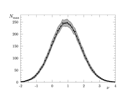
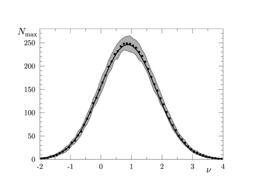
Figure 1: The ensemble average of Nmax(ν)subscript𝑁max𝜈N_{\hbox{\scriptsize max}}(\nu) for the ΛΛ\LambdaCDM concordance model computed by Eq. (13) is shown as a solid line. Panel (a) compares this curve with the average of Nmax(ν)subscript𝑁max𝜈N_{\hbox{\scriptsize max}}(\nu) computed from 50 realisations of the infinite volume model (circles). Panel (b) shows the result obtained from 50 realisations of the torus universe with the side length L=3.86LH𝐿3.86subscript𝐿𝐻L=3.86\,L_{H} (circles). To reveal the cosmic variance, the 1σ1𝜎1\sigma standard deviation is displayed as a grey band which is calculated from the corresponding 50 maps.

For a homogeneous and isotropic Gaussian random field, the distribution Nmax(ν)subscript𝑁max𝜈N_{\hbox{\scriptsize max}}(\nu) is given by

Nmax(ν)=1(2π)32θ2exp[ν22]G(ν,γ,α)subscript𝑁max𝜈1superscript2𝜋32superscript𝜃absent2superscript𝜈22𝐺𝜈𝛾𝛼N_{\hbox{\scriptsize max}}(\nu)=\frac{1}{(2\pi)^{\frac{3}{2}}\,\theta^{*2}}\exp\left[-\frac{\nu^{2}}{2}\right]\,G(\nu,\gamma,\alpha)\hskip 5.0pt (13)

with

G(ν,γ,α)𝐺𝜈𝛾𝛼\displaystyle G(\nu,\gamma,\alpha) :=assign\displaystyle:= γν(1γ2)exp[γ2ν22(1γ2)]2π(1γ2)𝛾𝜈1superscript𝛾2superscript𝛾2superscript𝜈221superscript𝛾22𝜋1superscript𝛾2\displaystyle\gamma\nu(1-\gamma^{2})\frac{\exp\left[-\frac{\gamma^{2}\,\nu^{2}}{2(1-\gamma^{2})}\right]}{\sqrt{2\,\pi\,(1-\gamma^{2})}}
+(α2(1γ2)1+γ2ν2)[112erfc(γν2(1γ2))]superscript𝛼21superscript𝛾21superscript𝛾2superscript𝜈2delimited-[]112erfc𝛾𝜈21superscript𝛾2\displaystyle+\left(\alpha^{2}(1-\gamma^{2})-1+\gamma^{2}\nu^{2}\right)\left[1-\frac{1}{2}\hbox{erfc}\left(\frac{\gamma\nu}{\sqrt{2(1-\gamma^{2})}}\right)\right]
+exp[α2γ2ν21+2α2(1γ2)]2α2(1γ2)+1[112erfc(γν2(1γ2)(1+2α2(1γ2)))],superscript𝛼2superscript𝛾2superscript𝜈212superscript𝛼21superscript𝛾22superscript𝛼21superscript𝛾21delimited-[]112erfc𝛾𝜈21superscript𝛾212superscript𝛼21superscript𝛾2\displaystyle+\frac{\exp\left[\frac{-\alpha^{2}\,\gamma^{2}\,\nu^{2}}{1+2\alpha^{2}(1-\gamma^{2})}\right]}{\sqrt{2\alpha^{2}(1-\gamma^{2})+1}}\left[1-\frac{1}{2}\hbox{erfc}\left(\frac{\gamma\nu}{\sqrt{2(1-\gamma^{2})(1+2\alpha^{2}(1-\gamma^{2}))}}\right)\right]\hskip 5.0pt,

and is derived in A.1, see Eq. (50). Here erfc(x)erfc𝑥\hbox{erfc}(x) is the complementary error function. The parameters are

α:=1+2σ12σ22,θ2:=α21=2σ12σ22,   andγ:=σ12σ2σ0α.\alpha:=\sqrt{1+\frac{2\sigma^{2}_{1}}{\sigma^{2}_{2}}}\hskip 10.0pt,\hskip 10.0pt\theta^{*2}:=\alpha^{2}-1=\frac{2\sigma^{2}_{1}}{\sigma^{2}_{2}}\hskip 10.0pt\hbox{, \; and}\hskip 10.0pt\gamma:=\frac{\sigma_{1}^{2}}{\sigma_{2}\,\sigma_{0}\,\alpha}\hskip 10.0pt. (14)

In Fig. 1 the theoretical distribution (13) is shown and compared with the mean value obtained from 50 CMB maps simulated at the HEALPix resolution Nside=512subscript𝑁side512N_{\hbox{\scriptsize side}}=512 using a smoothing of 1superscript11^{\circ} and l1000𝑙1000l\leq 1000. Both panels are based on the cosmological parameters of the infinite volume best-fit ΛΛ\LambdaCDM model of the WMAP data. In panel (a) the infinite model, which is isotropic, is shown, whereas panel (b) shows a multi-connected model which is anisotropic and thus does not fulfil the assumptions on which (13) is based. However, as revealed by Fig. 1(b) the data points match the distribution (13) with the same quality as in Fig. 1(a). In addition, the 50 realisations can be used to get an estimate of the cosmic variance. The corresponding 1σ1𝜎1\sigma standard deviation is displayed as a grey band in Fig. 1. The results for the mean value and the variance of Nmax(ν)subscript𝑁max𝜈N_{\hbox{\scriptsize max}}(\nu) for the torus universe are almost the same as for the infinite one. One could have expected this result since the number of maxima is primarily determined by the smallest scales, and a multi-connected model, which possesses in the shown case a cubic topology with a side length L=3.86LH𝐿3.86subscript𝐿𝐻L=3.86\,L_{H}, differs from the infinite one only on very large scales. Similar results are also expected in the case of other topologies, homogeneous and inhomogeneous manifolds, if the topological scales of the universe are of comparable order. Only if the volume of the universe is much smaller than the volume inside the surface of last scattering, one can expect any differences in the Nmaxsubscript𝑁maxN_{\hbox{\scriptsize max}} distribution to those calculated in A.1. In such a case one would get an influence of the topology on small scales. But until now no hint is found in the data for a model with such a sufficiently small volume.

Refer to captionRefer to caption

(a)

4πθ2Nmax4𝜋superscript𝜃absent2subscript𝑁max4\pi\theta^{*2}\,N_{\hbox{\scriptsize max}}

α𝛼\alpha(b)α𝛼\alphaσfwhmsubscript𝜎fwhm\sigma_{\hbox{\scriptsize fwhm}}[deg]

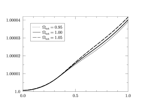
Figure 2: In panel (a) the formula of the total number Nmaxsubscript𝑁maxN_{\hbox{\scriptsize max}} of maxima per solid angle resulting from Equation (A1.7) in Ref. \refciteBond_Efstathiou_1987 (solid line) is compared to our Eq. (15) (dashed line). In panel (b) the parameter α𝛼\alpha is plotted as a function of the smoothing scale σfwhmsubscript𝜎fwhm\sigma_{\hbox{\scriptsize fwhm}} for three cosmological models. All values of α𝛼\alpha are very close to one.

Our formulae for the various Nmaxsubscript𝑁maxN_{\hbox{\scriptsize max}} distributions in A.1 differ by terms depending on the parameter α𝛼\alpha from the corresponding equations in Ref. \refciteBond_Efstathiou_1987. Here these differences are discussed using the example of the total number of maxima per solid angle. Our formula to this quantity is given by

Nmaxsubscript𝑁max\displaystyle N_{\hbox{\scriptsize max}} =\displaystyle= NmaxB&E[(α21)1+2α2+1]31+2α2superscriptsubscript𝑁maxB&Edelimited-[]superscript𝛼2112superscript𝛼21312superscript𝛼2\displaystyle N_{\hbox{\scriptsize max}}^{\hbox{\scriptsize B\&E}}\,\frac{\left[\left(\alpha^{2}-1\right)\sqrt{1+2\alpha^{2}}+1\right]\sqrt{3}}{\sqrt{1+2\alpha^{2}}}\hskip 5.0pt (15)

which is derived in A.1, see (46). The corresponding result obtained from Equation (A1.7) in Ref. \refciteBond_Efstathiou_1987 is NmaxB&E=14πθ23superscriptsubscript𝑁maxB&E14𝜋superscript𝜃absent23N_{\hbox{\scriptsize max}}^{\hbox{\scriptsize B\&E}}=\frac{1}{4\pi\theta^{*2}\sqrt{3}}, which is the leading term of the Laurent series of our Eq. (15) at α2=1superscript𝛼21\alpha^{2}=1. Both formulae are compared in Fig. 2(a) where 4πθ2Nmax4𝜋superscript𝜃absent2subscript𝑁max4\pi\theta^{*2}\,N_{\hbox{\scriptsize max}} is displayed. In the case of NmaxB&Esuperscriptsubscript𝑁maxB&EN_{\hbox{\scriptsize max}}^{\hbox{\scriptsize B\&E}} an α𝛼\alpha-independent, i. e. model independent value of 1313\frac{1}{\sqrt{3}} is obtained. In contrast our result for 4πθ2Nmax4𝜋superscript𝜃absent2subscript𝑁max4\pi\theta^{*2}\,N_{\hbox{\scriptsize max}} depends on α𝛼\alpha and therefore on the cosmological model since α𝛼\alpha, σ12superscriptsubscript𝜎12\sigma_{1}^{2} and σ22superscriptsubscript𝜎22\sigma_{2}^{2} depend on the angular power spectrum. In Fig. 2(a) we have varied α[1,2]𝛼12\alpha\in[1,2] in order to demonstrate the difference between Nmaxsubscript𝑁maxN_{\hbox{\scriptsize max}} and the leading term NmaxB&Esuperscriptsubscript𝑁maxB&EN_{\hbox{\scriptsize max}}^{\hbox{\scriptsize B\&E}}. Is this interval of α𝛼\alpha realistic for cosmological models compatible with the measured data? To answer this question we have calculated σ12superscriptsubscript𝜎12\sigma_{1}^{2} and σ22superscriptsubscript𝜎22\sigma_{2}^{2} with a cut-off at l=1000𝑙1000l=1000 with the angular power spectrum of the best-fit ΛΛ\LambdaCDM model of the WMAP data. In addition, these parameters are computed from the angular power spectrum of two models with positive and negative curvature, where the cosmological constant is varied and the other cosmological parameters are held fixed. These three cosmological models lead to different values of α𝛼\alpha, whose dependence on the smoothing scale is displayed in Fig. 2(b). One observes that α𝛼\alpha is almost equal to 1, and thus θ2superscript𝜃absent2\theta^{*2} is very small for all realistic cosmological parameters and smoothing scales. Therefore, we conclude that for all practical purposes the additional dependence of 4πθ2Nmax4𝜋superscript𝜃absent2subscript𝑁max4\pi\theta^{*2}\,N_{\hbox{\scriptsize max}} on α𝛼\alpha is without relevance and the formulae of the Nmaxsubscript𝑁maxN_{\hbox{\scriptsize max}} distributions in Ref. \refciteBond_Efstathiou_1987 are adequate.

4.2 Elongation at Maxima and Minima

Now we turn to the elongation measure e𝑒e at maxima and minima. The ensemble average and the corresponding second moment of this quantity are given by

e=2α2+3321+2α22α2ln[1+2α21+2α212α21+2α2]4[(α21)1+2α2+1]delimited-⟨⟩𝑒2superscript𝛼233212superscript𝛼22superscript𝛼212superscript𝛼212superscript𝛼212superscript𝛼212superscript𝛼24delimited-[]superscript𝛼2112superscript𝛼21\displaystyle\langle e\rangle\;=\;\frac{2\alpha^{2}+3-\frac{3}{2}\sqrt{\frac{1+2\alpha^{2}}{2\alpha^{2}}}\ln\left[\frac{1+\sqrt{\frac{2\alpha^{2}}{1+2\alpha^{2}}}}{1-\sqrt{\frac{2\alpha^{2}}{1+2\alpha^{2}}}}\right]}{4\left[(\alpha^{2}-1)\sqrt{1+2\alpha^{2}}+1\right]}\hskip 5.0pt (16)

and

e2=131+2α2+4(1+2α21)(1+2α22α2)4[(α21)1+2α2+1],delimited-⟨⟩superscript𝑒21312superscript𝛼2412superscript𝛼2112superscript𝛼22superscript𝛼24delimited-[]superscript𝛼2112superscript𝛼21\displaystyle\langle e^{2}\rangle\;=\;\frac{1-3\,\sqrt{1+2\alpha^{2}}+4(\sqrt{1+2\alpha^{2}}-1)\left(\frac{1+2\alpha^{2}}{2\alpha^{2}}\right)}{4\left[(\alpha^{2}-1)\sqrt{1+2\alpha^{2}}+1\right]}\hskip 5.0pt, (17)

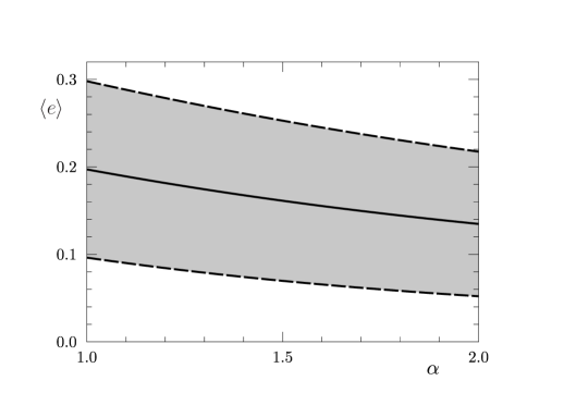
which both depend on the parameter α𝛼\alpha. The formulae are derived in the A.2. The mean value of the elongation e𝑒e together with the standard deviation due to the cosmic variance is displayed in panel (a) of Fig. 3. The distribution

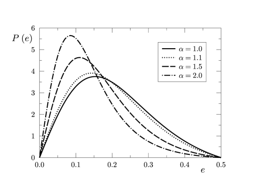
P(e)=24e(14e2)α41+2α2(1+8α2e2)52[(α21)1+2α2+1]𝑃𝑒24𝑒14superscript𝑒2superscript𝛼412superscript𝛼2superscript18superscript𝛼2superscript𝑒252delimited-[]superscript𝛼2112superscript𝛼21\displaystyle P(e)\;=\;\frac{24\,e(1-4e^{2})\alpha^{4}\sqrt{1+2\alpha^{2}}}{\left(1+8\alpha^{2}e^{2}\right)^{\frac{5}{2}}\left[(\alpha^{2}-1)\sqrt{1+2\alpha^{2}}+1\right]}\hskip 5.0pt (18)

of the elongation is plotted for four values of α𝛼\alpha in Fig. 3(b). This demonstrates that P(e)𝑃𝑒P(e) depends on the parameter α𝛼\alpha and thus in turn via the angular power spectrum on the cosmological parameters. In this way the elongation measure e𝑒e encodes some properties of the Universe.
Refer to captionRefer to caption

(a)(b)

Figure 3: In panel (a) the ensemble average of the elongation e𝑒e with the corresponding 1σ1𝜎1\sigma standard deviation is displayed depending on the parameter α𝛼\alpha. In panel (b) the distribution P(e)𝑃𝑒P(e) of the elongation e𝑒e is plotted depending on the parameter α𝛼\alpha.

This dependence of the elongation e𝑒e on cosmological parameters is not discussed in Ref. \refciteBond_Efstathiou_1987. In currently admissible cosmological models the dependence on α𝛼\alpha in (A.2) can be neglected since the corresponding values of α𝛼\alpha are very close to one. The ensemble average of the elongation e𝑒e is approximatively given by 0.197 for α=1𝛼1\alpha=1. Similar results are obtained for the other elongation measures, i. e. for the ellipticity E𝐸E and the eccentricity ε𝜀\varepsilon. The ensemble averages of these quantities are given by (63) and (60). Their values are approximately E1.648𝐸1.648E\approx 1.648 and ε0.715𝜀0.715\varepsilon\approx 0.715 independent from the model. The cosmological influence on the elongation e𝑒e, the ellipticity E𝐸E or the eccentricity ε𝜀\varepsilon is very difficult to measure. The difficulty arises from the large cosmic variance for these quantities which is displayed as a grey band in Fig. 3(a) in the case of the elongation e𝑒e. Furthermore, also the detector noise and the foregrounds in a sky map obtained by observations have an influence on the elongation, but this will be discussed later.

In addition, it is not expected that the topology of the Universe, i. e. a multi-connected spatial space, can influence the elongation of contour lines since the volumes of the fundamental cells are too large. Nevertheless, several measures of the elongation are discussed below for the special case of the cubic topology which is motivated by the fact that this model is statistically anisotropic.

5 Elongation of Hot and Cold Spots

There are different algorithms to compute the ellipticity. One method is based on the Taylor expansion of the temperature field at local maxima or minima as used in the Appendix. Alternatively, the ellipticity can be calculated by using an “inertia” tensor as described in the following.

5.1 Computation of the ellipticity

In the following the normalised temperature field

u(n^)=δTFl(n^)σ0𝑢^𝑛𝛿subscript𝑇subscript𝐹𝑙^𝑛subscript𝜎0u(\hat{n})\;=\;\frac{\delta T_{F_{l}}(\hat{n})}{\sigma_{0}} (19)

is used. In the theoretical derivation which is outlined in the Appendix, this σ0subscript𝜎0\sigma_{0} is obtained by the ensemble average by using σ0=C(0)subscript𝜎0𝐶0\sigma_{0}=\sqrt{C(0)} where C(0)𝐶0C(0) is the 2-point correlation function of the CMB at a separation angle ϑ=0italic-ϑ0\vartheta=0. Such an ensemble average is not possible for a CMB sky map obtained by observations, of course, since there is only a single CMB sky from our point of view. Therefore, a sky map analysis computes the value of σ0subscript𝜎0\sigma_{0} from a given single sky realisation as the usual standard deviation of the temperature field

σ0=NδΩ1δΩ(δTFl(n^)T¯)2𝑑Ω,subscript𝜎0superscriptsubscript𝑁𝛿Ω1subscript𝛿Ωsuperscript𝛿subscript𝑇subscript𝐹𝑙^𝑛¯𝑇2differential-dΩ\sigma_{0}=\sqrt{N_{\delta\Omega}^{-1}\int_{\delta\Omega}(\delta T_{F_{l}}(\hat{n})-\bar{T})^{2}d\Omega}\hskip 10.0pt, (20)

where T¯¯𝑇\bar{T} is the mean temperature. In the analysis of masked maps the observed area is δΩ𝛿Ω\delta\Omega and NδΩsubscript𝑁𝛿ΩN_{\delta\Omega} is the fraction of the sky that is not masked.

To get a binary image we define the excursion set of hot spots (HS) by

QνHS={n^𝕊2|u(n^)ν}.superscriptsubscript𝑄𝜈HSconditional-set^𝑛superscript𝕊2𝑢^𝑛𝜈Q_{\nu}^{\hbox{\scriptsize HS}}\;=\;\left\{\hat{n}\in\mathbb{S}^{2}|u(\hat{n})\geq\nu\right\}\hskip 10.0pt. (21)

Here one excludes all regions with a temperature value lower than the value of the threshold ν𝜈\nu. Analogously the excursion set of cold spots (CS) is defined by

QνCS={n^𝕊2|u(n^)ν}.superscriptsubscript𝑄𝜈CSconditional-set^𝑛superscript𝕊2𝑢^𝑛𝜈Q_{\nu}^{\hbox{\scriptsize CS}}\;=\;\left\{\hat{n}\in\mathbb{S}^{2}|u(\hat{n})\leq\nu\right\}\hskip 10.0pt. (22)

The multi-connected set Qνsubscript𝑄𝜈Q_{\nu} can be interpreted as the union

Qν=i=1NνQνisubscript𝑄𝜈superscriptsubscript𝑖1subscript𝑁𝜈superscriptsubscript𝑄𝜈𝑖Q_{\nu}\;=\;\bigcup\limits_{i=1}^{N_{\nu}}Q_{\nu}^{i} (23)

of the Nνsubscript𝑁𝜈N_{\nu} simply connected spots Qνisuperscriptsubscript𝑄𝜈𝑖Q_{\nu}^{i}. We compute the ellipticity for every spot Qνisuperscriptsubscript𝑄𝜈𝑖Q_{\nu}^{i} by using the inertia tensor defined by

I(Qνi):=(IxxIxyIyxIyy)=(y2dxdyyxdxdyxydxdyx2dxdy).assign𝐼superscriptsubscript𝑄𝜈𝑖fragmentsI𝑥𝑥fragmentsI𝑥𝑦fragmentsI𝑦𝑥fragmentsI𝑦𝑦fragmentsy2dxdyfragmentsyxdxdyfragmentsxydxdyfragmentsx2dxdyI(Q_{\nu}^{i})\;:=\;\left(\begin{tabular}[]{rr}$I_{xx}$&$I_{xy}$\\ $I_{yx}$&$I_{yy}$\end{tabular}\right)\;=\;\left(\begin{tabular}[]{rr}$\int\int y^{2}dxdy$&$-\int\int yx\,dxdy$\\ $-\int\int xy\,dxdy$&$\int\int x^{2}dxdy$\end{tabular}\right)\hskip 10.0pt. (24)

The spots are projected onto the xy𝑥𝑦xy-plane where the origin of the coordinate system matches the centre of mass of the spot Qνisuperscriptsubscript𝑄𝜈𝑖Q_{\nu}^{i}. The symmetric tensor I(Qνi)𝐼superscriptsubscript𝑄𝜈𝑖I(Q_{\nu}^{i}) has two real eigenvalues λ1subscript𝜆1\lambda_{1} and λ2subscript𝜆2\lambda_{2} whose relation to the ellipticity E𝐸E is given by

E(Qνi)=λ1λ2.𝐸superscriptsubscript𝑄𝜈𝑖subscript𝜆1subscript𝜆2E(Q_{\nu}^{i})\;=\;\sqrt{\frac{\lambda_{1}}{\lambda_{2}}}\hskip 10.0pt. (25)

For the special case of an ellipse with axes a𝑎a and b𝑏b the eigenvalues can be computed to be

λ1=π4a3b and λ2=π4ab3 with λ1λ2.formulae-sequencesubscript𝜆1𝜋4superscript𝑎3𝑏 and formulae-sequencesubscript𝜆2𝜋4𝑎superscript𝑏3 with subscript𝜆1subscript𝜆2\lambda_{1}\;=\;\frac{\pi}{4}\,a^{3}\,b\hskip 10.0pt\hbox{ and }\hskip 10.0pt\lambda_{2}\;=\;\frac{\pi}{4}\,a\,b^{3}\hskip 10.0pt\hbox{ with }\hskip 10.0pt\lambda_{1}\geq\lambda_{2}\hskip 10.0pt. (26)

Inserting this into (25) leads back to the definition (1), respectively (9) of the ellipticity

E=ab=λ1λ2.𝐸𝑎𝑏subscript𝜆1subscript𝜆2E\;=\;\frac{a}{b}\;=\;\sqrt{\frac{\lambda_{1}}{\lambda_{2}}}\hskip 10.0pt. (27)

The other quantities for elongation given in (10) and (11) can be obtained from the conversion formulae. The true niveau lines are not perfect ellipses, of course, but the above prescription can be used in order to obtain the ellipticity of that ellipse which approximates best the niveau line. Since there are niveau lines which deviate strongly from an ellipse one needs a further criterion to eliminate such curves in order to avoid non-sense results.

5.2 The dependence of the ellipticity on the resolution

The ellipticity depends sensitively on the accuracy of the sky map and care has to be taken with respect to the resolution of the map, the beam profile and the noise properties. In so far, it is not a very robust measure to characterise the CMB sky, and the details of the computation of the ellipticity have to be defined clearly in order to obtain reproducible values.
Refer to captionRefer to caption

(a)(b)

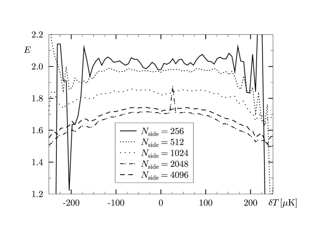
Figure 4: The ellipticity E𝐸E is computed for a realisation of the cubic universe as described in the text based on the cosmological parameters of the concordance model. The dependence on the value of Nsidesubscript𝑁sideN_{\hbox{\scriptsize side}} is presented. Panel (a) shows the ellipticity E𝐸E where all contours are taken into account that enclose at least 10 pixels. The ellipticity E𝐸E increases with decreasing Nsidesubscript𝑁sideN_{\hbox{\scriptsize side}}. In Panel (b) all contours are selected enclosing an area of at least 0.525deg20.525superscriptdeg20.525\,\hbox{deg}^{2}.

Let us at first address the issue of the resolution of the sky map. The CMB sky maps are usually stored in the HEALPix[18] format whose resolution is determined by the parameter Nsidesubscript𝑁sideN_{\hbox{\scriptsize side}}. In order to determine the dependence of the ellipticity E𝐸E on the value of Nsidesubscript𝑁sideN_{\hbox{\scriptsize side}}, a sky map is simulated for the cubic topology using the cosmological parameters of the ΛΛ\LambdaCDM concordance model. We start with a highest resolution of Nside=4096subscript𝑁side4096N_{\hbox{\scriptsize side}}=4096. The sky maps are normalised such that the temperature fluctuations possess a standard deviation of 66μK66𝜇K66\mu\hbox{K}, which is the value obtained from the five-year ILC map outside the KQ75 mask.

For such a simulation the ellipticity E𝐸E is computed for the contour lines of a given temperature threshold δT𝛿𝑇\delta T, and the mean value is shown in Fig. 4. Contour lines that are too small are excluded since they are determined by very few pixels such that the ellipticity E𝐸E is ill defined. In Fig. 4(a) the criterion is that the contour lines should at least circumference 10 pixels with respect to the chosen resolution Nsidesubscript𝑁sideN_{\hbox{\scriptsize side}}. This implies that ever more small contour lines are taken into account as the value of Nsidesubscript𝑁sideN_{\hbox{\scriptsize side}} increases. Thus the mean values are computed from different sets of contour lines. This contrasts to the criterion of a fixed minimal area which leads to the result displayed in Fig. 4(b). There, all contour lines are taken into account which are larger than 10 pixels with respect to the Nside=256subscript𝑁side256N_{\hbox{\scriptsize side}}=256 resolution, i. e. all contours encompassing an area larger than 0.525deg20.525superscriptdeg20.525\,\hbox{deg}^{2}. Thus the curve belonging to Nside=256subscript𝑁side256N_{\hbox{\scriptsize side}}=256 is the same in both panels. Whereas the exclusion criterion of a fixed pixel number leads to a robust estimation of E𝐸E only at very large values of Nsidesubscript𝑁sideN_{\hbox{\scriptsize side}}, the exclusion criterion of a fixed area gives consistent values already for values of Nsidesubscript𝑁sideN_{\hbox{\scriptsize side}} as small as 512. But recall from Section 4.2 that the expected ellipticity is E1.648similar-to-or-equals𝐸1.648E\simeq 1.648 for a Gaussian field. This value is, however, obtained with the first selection criterion which takes an increasing number of contour lines into account. This analysis thus favours the first selection criterion and, furthermore, demonstrates the sensitivity of the elongation measures.
Refer to caption
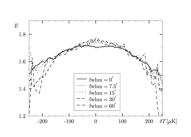
Figure 5: For the CMB simulation used in Fig. 4(a) having the HEALPix resolution of Nside=4096subscript𝑁side4096N_{\hbox{\scriptsize side}}=4096, the ellipticity E𝐸E is shown in dependence on the width of the Gaussian beam.

The dependence of the ellipticity on the smoothing is not very strong. This can be inferred from Fig. 2(b) where the value of α𝛼\alpha is plotted as a function of the smoothing σfwhmsubscript𝜎fwhm\sigma_{\hbox{\scriptsize fwhm}}. Up to a smoothing of 1 degree all values of α𝛼\alpha are below 1.00004 and the expectation value for the ellipticity E𝐸E, Eq. (63), is nearly constant for these smoothings. This behaviour is confirmed in Fig. 5 where different smoothings are applied to the sky maps with a fixed HEALPix resolution of Nside=4096subscript𝑁side4096N_{\hbox{\scriptsize side}}=4096.

5.3 The dependence of the elongation on the curvature

Let us now turn to the dependence of the elongation on the curvature which is claimed[7, 8, 9, 10, 11, 12] to be sufficiently strong in order to reveal the curvature of the Universe. However, in Ref. \refciteBarreiro_Sanz_Martinez-Gonzalez_Cayon_Silk_1997 no such ellipticity-curvature correlation is found. Since the elongations depend on the parameter α𝛼\alpha and thus on the cosmological parameters, such a correlation could exist. The discussion in the previous section has shown that the elongation depends on the size of the niveau lines which have to enclose at least nminsubscript𝑛minn_{\hbox{\scriptsize min}} pixels. For the computation of the elongation our algorithm requires at least an area greater than 444 pixels. The number of niveau lines which can be used in a statistic depends on the normalised temperature ν𝜈\nu. It is maximal at ν=±1𝜈plus-or-minus1\nu=\pm 1 where the number Nνsubscript𝑁𝜈N_{\nu} of spots has its maximum. The values of nminsubscript𝑛minn_{\hbox{\scriptsize min}} and of the normalised temperature ν𝜈\nu are required to specify the mean ellipticity E¯(ν,nmin)¯𝐸𝜈subscript𝑛min\bar{E}(\nu,n_{\hbox{\scriptsize min}}).

The ensemble average of the elongation and the corresponding cosmic variance are computed from an ensemble of 1000 sky realisations. We analyse the excursion sets Qνsubscript𝑄𝜈Q_{\nu} for hot spots with thresholds ν>0𝜈0\nu>0 and for cold spots with thresholds ν<0𝜈0\nu<0. We get for every threshold ν𝜈\nu an amount of Nνsubscript𝑁𝜈N_{\nu} spots with individual areas n(Qνi)𝑛superscriptsubscript𝑄𝜈𝑖n(Q_{\nu}^{i}) and elongations e(Qνi)𝑒superscriptsubscript𝑄𝜈𝑖e(Q_{\nu}^{i}). The mean ellipticity E¯(ν,nmin)¯𝐸𝜈subscript𝑛min\bar{E}(\nu,n_{\hbox{\scriptsize min}}) is computed at ν=1𝜈1\nu=1 by averaging the values of all spots with n>nmin𝑛subscript𝑛minn>n_{\hbox{\scriptsize min}}. This method is used in Refs. \refciteGurzadyan_et_al_2003b,Gurzadyan_et_al_2004,Gurzadyan_et_al_2005,Gurzadya_et_al_2007. An alternative averaging is used for the mean elongation e¯(ν,n,Δn)¯𝑒𝜈𝑛Δ𝑛\bar{e}(\nu,n,\Delta n) which is computed as a moving average around a spot size n𝑛n, i. e. from spots having pixel numbers within the interval [nΔn,n+Δn]𝑛Δ𝑛𝑛Δ𝑛\left[n-\Delta n,n+\Delta n\right]. Our examination shows that these mean values are very stable with respect to the choice of the threshold ν𝜈\nu in a range of ν[2,2]𝜈22\nu\in\left[-2,2\right].

Refer to captionRefer to caption

σfwhm=20 arcminsubscript𝜎fwhm20 arcmin{\sigma}_{\hbox{\scriptsize fwhm}}=20\hbox{ arcmin}σfwhm=20 arcminsubscript𝜎fwhm20 arcmin{\sigma}_{\hbox{\scriptsize fwhm}}=20\hbox{ arcmin}E¯¯𝐸\bar{E}nminsubscript𝑛minn_{\hbox{\scriptsize min}}e¯¯𝑒\bar{e}n𝑛n
Refer to captionRefer to caption
σfwhm=40 arcminsubscript𝜎fwhm40 arcmin{\sigma}_{\hbox{\scriptsize fwhm}}=40\hbox{ arcmin}σfwhm=40 arcminsubscript𝜎fwhm40 arcmin{\sigma}_{\hbox{\scriptsize fwhm}}=40\hbox{ arcmin}E¯¯𝐸\bar{E}nminsubscript𝑛minn_{\hbox{\scriptsize min}}e¯¯𝑒\bar{e}n𝑛n
Refer to captionRefer to caption
σfwhm=60 arcminsubscript𝜎fwhm60 arcmin{\sigma}_{\hbox{\scriptsize fwhm}}=60\hbox{ arcmin}σfwhm=60 arcminsubscript𝜎fwhm60 arcmin{\sigma}_{\hbox{\scriptsize fwhm}}=60\hbox{ arcmin}E¯¯𝐸\bar{E}nminsubscript𝑛minn_{\hbox{\scriptsize min}}e¯¯𝑒\bar{e}n𝑛n

Figure 6: The ensemble average of the mean ellipticity E¯(ν,nmin)¯𝐸𝜈subscript𝑛min\bar{E}(\nu,n_{\hbox{\scriptsize min}}) with ν=1𝜈1\nu=1 (left) and the mean elongation e¯(ν,n,Δn)¯𝑒𝜈𝑛Δ𝑛\bar{e}(\nu,n,\Delta n) with ν=1𝜈1\nu=1 and Δn=20Δ𝑛20\Delta n=20 pixels (right) is computed using three Gaussian smoothing kernels (from top to bottom: σfwhm=20 arcminsubscript𝜎fwhm20 arcmin{\sigma}_{\hbox{\scriptsize fwhm}}=20\hbox{ arcmin}, 40 arcmin40 arcmin40\hbox{ arcmin}, and 60 arcmin60 arcmin60\hbox{ arcmin}). The grey bands reflect the cosmic variance of the flat ΛΛ\LambdaCDM concordance model. The ensemble average is computed from 1000 realisations. The sky maps have a resolution of Nside=512subscript𝑁side512N_{\hbox{\scriptsize side}}=512.

In Fig. 6 the ensemble average of the mean ellipticity E¯(ν,nmin)¯𝐸𝜈subscript𝑛min\bar{E}(\nu,n_{\hbox{\scriptsize min}}) with ν=1𝜈1\nu=1 (left) and the mean elongation e¯(ν,n,Δn)¯𝑒𝜈𝑛Δ𝑛\bar{e}(\nu,n,\Delta n) with ν=1𝜈1\nu=1 and Δn=20Δ𝑛20\Delta n=20 pixels (right) is shown. The average is computed from 1000 realisations. The sky maps possess a resolution of Nside=512subscript𝑁side512N_{\hbox{\scriptsize side}}=512 and lmax=1000subscript𝑙max1000l_{\hbox{\scriptsize max}}=1000. The grey band reflects the cosmic variance of the flat ΛΛ\LambdaCDM concordance model (solid line). This provides the criterion whether two cosmological models can be distinguished by an elongation measure. In order to distinguish them the corresponding curves should deviate more than the width of the band due to the cosmic variance. Note that in contrast to the previous figures, the Fig. 6 displays the elongation as a function of the spot size and not of the temperature to which the niveau lines belong. This kind of plotting reveals the remarkable fact that larger spots possess a higher degree of elongation than smaller ones. This dependence is not covered by our analytical formulae which are based on the infinitesimal neighbourhood at maxima or minima. The impact of three Gaussian smoothing kernels is also investigated in Fig. 6 (from top to bottom: σfwhm=20,40,60 arcminsubscript𝜎fwhm204060 arcmin{\sigma}_{\hbox{\scriptsize fwhm}}=20,40,60\hbox{ arcmin}). An increased smoothing reduces the degree of elongation. This is due to the symmetric smoothing kernel which rounds off the structures. Here the resolution of Nside=512subscript𝑁side512N_{\hbox{\scriptsize side}}=512 does not resolve all physical structures of the Gaussian temperature field. This contrasts to Fig. 5 which is based on a sky map with a resolution of Nside=4096subscript𝑁side4096N_{\hbox{\scriptsize side}}=4096 being sufficiently fine grained to resolve all structures such that the analytical formulae are applicable.

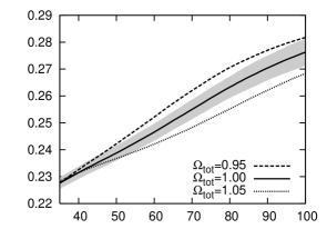
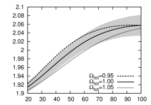
In Fig. 6 the ensemble average of the elongations is plotted for three cosmological models which differ with respect to their curvature. In addition to the flat ΛΛ\LambdaCDM concordance model, the ensemble average of a positively curved universe (dotted line) and a negatively curved universe (dashed line) is displayed. The figure reveals that a universe with negative curvature possesses a larger degree of elongation for a given spot size than the flat universe. This trend is continued for a universe with positive curvature which possesses a smaller degree of elongation for a given spot size than the flat universe. This encouraging behaviour could be used to distinguish different cosmological models if their corresponding curves differ by more than the scattering due to the cosmic variance. It turns out that this depends on the resolution of the sky maps. By applying wider smoothing kernels (from top to bottom in Fig. 6) the differences between the curves decrease and are getting insignificant compared to the cosmic variance for smoothings around σfwhm=60 arcminsubscript𝜎fwhm60 arcmin\sigma_{\hbox{\scriptsize fwhm}}=60\hbox{ arcmin}. Note that the mean elongation e¯(ν,n,Δn)¯𝑒𝜈𝑛Δ𝑛\bar{e}(\nu,n,\Delta n) based on a moving average does a better job than the mean ellipticity E¯(ν,nmin)¯𝐸𝜈subscript𝑛min\bar{E}(\nu,n_{\hbox{\scriptsize min}}). This is caused by the fact that the differences in the elongation vanish for spots with a large area, and thereby their inclusion blurs the signal. The figure reveals that a resolution of at least σfwhm=20 arcminsubscript𝜎fwhm20 arcmin\sigma_{\hbox{\scriptsize fwhm}}=20\hbox{ arcmin} is necessary in order to distinguish between cosmological models having a difference in curvature of ΔΩtot=0.05ΔsubscriptΩtot0.05\Delta\Omega_{\hbox{\scriptsize tot}}=0.05. This excludes the application of the ILC sky map of the WMAP team which has a resolution of about σfwhm=60 arcminsubscript𝜎fwhm60 arcmin\sigma_{\hbox{\scriptsize fwhm}}=60\hbox{ arcmin}. Better resolved sky maps such as the W-band maps of the WMAP team are available but they are contaminated with noise. Hence we now focus on the influence of noise on the elongation measures.
Refer to captionRefer to caption

without noisewithout noiseE¯¯𝐸\bar{E}nminsubscript𝑛minn_{\hbox{\scriptsize min}}e¯¯𝑒\bar{e}n𝑛n
Refer to captionRefer to caption
with noisewith noiseE¯¯𝐸\bar{E}nminsubscript𝑛minn_{\hbox{\scriptsize min}}e¯¯𝑒\bar{e}n𝑛n
Refer to captionRefer to caption
E¯¯𝐸\bar{E}nminsubscript𝑛minn_{\hbox{\scriptsize min}}e¯¯𝑒\bar{e}n𝑛n

Figure 7: The ensemble average of the mean ellipticity E¯(ν,nmin)¯𝐸𝜈subscript𝑛min\bar{E}(\nu,n_{\hbox{\scriptsize min}}) with ν=1𝜈1\nu=1 (left) and of the mean elongation e¯(ν,n,Δn)¯𝑒𝜈𝑛Δ𝑛\bar{e}(\nu,n,\Delta n) with ν=1𝜈1\nu=1 and Δn=20Δ𝑛20\Delta n=20 pixels (right) is presented. These curves are obtained from 1000 sky simulations which take the window function of the W-band (channel 4) of WMAP into account. The grey bands reflect the cosmic variance of the flat ΛΛ\LambdaCDM concordance model (solid curve). The three rows give the results without noise (top), with noise (middle) and a comparison of both cases for the flat ΛΛ\LambdaCDM concordance model (bottom). The sky maps have a resolution of Nside=512subscript𝑁side512N_{\hbox{\scriptsize side}}=512.

In order to address the question whether the W-band maps are suitable for an elongation analysis, 1000 sky maps are simulated which take into account the explicit window function of the W-band (channel 4) of WMAP[20]. In Fig. 7 the ensemble averages obtained from such sky maps are shown for the mean ellipticity E¯(ν,nmin)¯𝐸𝜈subscript𝑛min\bar{E}(\nu,n_{\hbox{\scriptsize min}}) with ν=1𝜈1\nu=1 (left) and for the mean elongation e¯(ν,n,Δn)¯𝑒𝜈𝑛Δ𝑛\bar{e}(\nu,n,\Delta n) with ν=1𝜈1\nu=1 and Δn=20Δ𝑛20\Delta n=20 pixels (right). Again the grey band reflects the cosmic variance of the flat ΛΛ\LambdaCDM concordance model (solid line). In addition, a positively curved universe (dotted line) and a negatively curved universe (dashed line) is displayed.

The upper row of Fig. 7 neglects noise completely and only takes the W-band window function into account. Both figures are similar to the two upper figures in Fig. 6 which have a resolution of σfwhm=20 arcminsubscript𝜎fwhm20 arcmin\sigma_{\hbox{\scriptsize fwhm}}=20\hbox{ arcmin} comparable to that of the W-band. The mean elongation e¯(ν,n,Δn)¯𝑒𝜈𝑛Δ𝑛\bar{e}(\nu,n,\Delta n) of spots with a small area reveals a saturation which is absent in Fig. 6. Furthermore, both elongation measures yield smaller values for spots with a larger area. This is caused by the application of the W-band window function which deviates strongly from a Gaussian. In the middle row of Fig. 7 the noise is taken into account which changes the behaviour drastically. No useful discrimination between the different curved models is possible any more. The lowest row in Fig. 7 shows a comparison for the ΛΛ\LambdaCDM concordance model with and without noise in one figure in order to emphasise the deteriorating effect of noise. A further analysis shows that an incomplete sky coverage additionally broadens the cosmic variance. Therefore, no comparison to measured data can be shown here.

Finally, we compare the infinite volume ΛΛ\LambdaCDM model with a statistically anisotropic multi-connected model for which we again choose the cubic topology with side length L=3.86LH𝐿3.86subscript𝐿𝐻L=3.86\,L_{H}. As already discussed in Section 4.1 the volume of the fundamental cell is a significant fraction of the volume inside the surface of last scattering. Therefore, only the largest angular scales are modified but not the fine structures which determine the elongation. In Fig. 8 the mean ellipticity E¯¯𝐸\bar{E} and the elongation e¯¯𝑒\bar{e} computed from 50 torus realisations are compared with the elongations of the infinite flat ΛΛ\LambdaCDM model. As expected the mean values are almost identical and their small differences are confined within the corresponding bands of cosmic variance. Thus, the anisotropy of the torus model is too weak to allow a discrimination between the models using the elongation measures.

Refer to captionRefer to caption

(a)(b)E¯¯𝐸\bar{E}nminsubscript𝑛minn_{\hbox{\scriptsize min}}e¯¯𝑒\bar{e}n𝑛n

Figure 8: The ensemble average of the mean ellipticity E¯(ν,nmin)¯𝐸𝜈subscript𝑛min\bar{E}(\nu,n_{\hbox{\scriptsize min}}) with ν=1𝜈1\nu=1 (left) and of the mean elongation e¯(ν,n,Δn)¯𝑒𝜈𝑛Δ𝑛\bar{e}(\nu,n,\Delta n) with ν=1𝜈1\nu=1 and Δn=20Δ𝑛20\Delta n=20 pixels (right) is presented. The elongations E𝐸E and e𝑒e of the infinite ΛΛ\LambdaCDM model are shown as a solid curve and its cosmic variance as a grey band calculated from 1000 realisations. The elongations of the torus universe with L=3.86LH𝐿3.86subscript𝐿𝐻L=3.86\,L_{H} are shown as error bars which represent the cosmic variance based on 50 sky simulations. In both cases the window function of the W-band (channel 4) of WMAP is taken into account, but the noise is neglected. The sky maps have a resolution of Nside=512subscript𝑁side512N_{\hbox{\scriptsize side}}=512.

In addition to the above investigations we also analysed our simulated sky maps at other thresholds ν𝜈\nu. Quantitatively our statements are equivalent for hot spots and cold spots which is due to the isotropy properties of the random field. So we restrict ourselves in this paper to hot spots only. Nevertheless, if a single realisation of a measured sky map is studied, both should be combined into one statistic for a better significance. Other thresholds ν𝜈\nu with ν±1𝜈plus-or-minus1\nu\neq\pm 1 possess a smaller number of spots and, therefore, lead to larger variances which is counterproductive in order to distinguish between cosmological models. Besides the mean values E¯(ν,nmin)¯𝐸𝜈subscript𝑛min\bar{E}(\nu,n_{\hbox{\scriptsize min}}) and e¯(ν,n,Δn)¯𝑒𝜈𝑛Δ𝑛\bar{e}(\nu,n,\Delta n) we also studied higher moments, higher central moments and their statistical interpretations. Since it turns out that the mean value provides the most robust measure we restrict our discussion to them here. The moving average applied in e¯(ν,n,Δn)¯𝑒𝜈𝑛Δ𝑛\bar{e}(\nu,n,\Delta n) leads to the best discrimination between cosmological models, but the additional parameter ΔnΔ𝑛\Delta n has to be chosen adequately, since too small values result in small spot numbers (lack on statistics) and too large values result in a blurring caused by large spots.

6 Summary

In this paper the structures of CMB sky maps are studied with respect to the crucial question whether these structures betray some information about the underlying cosmological model. There are various quantities to analyse the structures of the niveau lines and the focus is put on the elongation which can be described by the ellipticity E𝐸E, Eq. (9), or the elongation measure e𝑒e defined in Eq. (11). The elongation depends on the parameter α𝛼\alpha, Eq. (14), which in turn depends on the multipole spectrum Clsubscript𝐶𝑙C_{l} and thus on the cosmology. The theoretical dependence of various elongation measures on α𝛼\alpha is given for the case that the statistical properties of the temperature field are those of two-dimensional homogeneous and isotropic Gaussian random fields. Our analysis leads to the conclusion that this dependence, however, is weak. Since the resolution of the maps has a superior influence on the niveau lines, the results obtained from sky maps depend on the pixelization and on the beam profile of the detector. Both deteriorating restrictions are analysed. It is found that the elongation cannot be analysed without reference to the pixelization and the beam profile.

The dependence of the elongation on the cosmological parameters can be investigated for niveau lines classified either by their temperature or by the area which they encompass. The curvature of the universe is revealed by the elongation as demonstrated in Fig. 6, where the elongation is considered as a function of the size of the spots. The best discrimination between cosmological models is obtained by applying the moving average to e¯(ν,n,Δn)¯𝑒𝜈𝑛Δ𝑛\bar{e}(\nu,n,\Delta n). A resolution of at least σfwhm=20 arcminsubscript𝜎fwhm20 arcmin\sigma_{\hbox{\scriptsize fwhm}}=20\hbox{ arcmin} is required in order to distinguish between cosmological models which differ in the curvature by ΔΩtot=0.05ΔsubscriptΩtot0.05\Delta\Omega_{\hbox{\scriptsize tot}}=0.05. This excludes the analysis of the ILC map of the WMAP team, whose resolution is three times lower. The required resolution is achieved by the W-band sky map which has, however, much stronger noise. The analysis of simulated maps with the noise properties of the W-band map shows that it is also not suitable for this investigation. The Planck mission will provide maps with a significantly higher resolution as well as lower noise such that there is the hope that the results of that mission can be analysed with respect to the structure properties of the CMB.

We also study the elongation properties of a multi-connected space form, i. e. a model of the universe having a non-trivial topology, because it is not statistically isotropic and thus violates the assumptions which have to be satisfied for the analytical expressions to be valid. No distinction is found between the trivial topology, i. e. the concordance model, and the non-trivial topology with respect to the elongation. This is expected since the topology modifies the physics on the largest scales and has thus only a modest influence on the elongation. At least as long as the fundamental cell is so large that it constitutes a significant fraction within the surface of last scattering. Thus the best prospects for elongation measures can be found in the detection of curvature.

Appendix A The Gaussian Random Field and the CMB

In this Appendix, we outline the derivation of the peak density and the ellipticity of the temperature fluctuations δT(n^)𝛿𝑇^𝑛\delta T\left(\hat{n}\right) of the CMB under the assumption that the temperature fluctuations behave as a homogeneous and isotropic Gaussian random field

f(δT(n^))=12πσ02exp(|δT(n^)|22σ02)𝑓𝛿𝑇^𝑛12𝜋superscriptsubscript𝜎02superscript𝛿𝑇^𝑛22superscriptsubscript𝜎02f\left(\delta T\left(\hat{n}\right)\right)=\frac{1}{\sqrt{2\pi\sigma_{0}^{2}}}\exp\left(-\frac{\left|\delta T\left(\hat{n}\right)\right|^{2}}{2\sigma_{0}^{2}}\right)\hskip 10.0pt (28)

on the 2-dimensional sphere. Here σ02(n^):=δT(n^)δT(n^)assignsuperscriptsubscript𝜎02^𝑛delimited-⟨⟩𝛿𝑇^𝑛𝛿𝑇^𝑛\sigma_{0}^{2}\left(\hat{n}\right):=\left\langle\delta T\left(\hat{n}\right)\delta T\left(\hat{n}\right)\right\rangle is the variance of the temperature fluctuations. In an isotropic model σ02superscriptsubscript𝜎02\sigma_{0}^{2} is independent of the direction n^^𝑛\hat{n} and is given in that case by

σ02=l(2l+1)4πCl|Fl|2=C(0).superscriptsubscript𝜎02subscript𝑙2𝑙14𝜋subscript𝐶𝑙superscriptsubscript𝐹𝑙2𝐶0\sigma_{0}^{2}=\sum_{l}\frac{\left(2l+1\right)}{4\pi}C_{l}\left|F_{l}\right|^{2}=C(0)\hskip 10.0pt. (29)

The ensemble average is specified as delimited-⟨⟩\langle...\rangle, Flsubscript𝐹𝑙F_{l} accounts for the appearance of a beam profile and C(0)𝐶0C(0) is the correlation function of the temperature fluctuations in a homogeneous and isotropic universe at a separation angle ϑ=0italic-ϑ0\vartheta=0. To use a compact notation in this Appendix, the subscript Flsubscript𝐹𝑙F_{l} at the temperature field δTFl𝛿subscript𝑇subscript𝐹𝑙\delta T_{F_{l}} is omitted. This index stands for the smoothing operation (6). The following derivations and notations are based on Ref. \refciteBond_Efstathiou_1987.

The temperature fluctuation δT(n^)𝛿𝑇^𝑛\delta T\left(\hat{n}\right) close to the direction n^superscript^𝑛\hat{n}^{\prime} on the 2-sphere is given by the Taylor series

δT(n^)𝛿𝑇^𝑛\displaystyle\delta T\left(\hat{n}\right) =\displaystyle= δT(n^)+[iδT(n^)]n^=n^(xixi)𝛿𝑇superscript^𝑛subscriptdelimited-[]subscript𝑖𝛿𝑇^𝑛^𝑛superscript^𝑛superscript𝑥𝑖superscript𝑥𝑖\displaystyle\delta T\left(\hat{n}^{\prime}\right)\;+\;\left[\nabla_{i}\delta T\left(\hat{n}\right)\right]_{\hat{n}=\hat{n}^{\prime}}(x^{i}-x^{\prime i}) (30)
+[ijδT(n^)]n^=n^2(xixi)(xjxj)+.subscriptdelimited-[]subscript𝑖subscript𝑗𝛿𝑇^𝑛^𝑛superscript^𝑛2superscript𝑥𝑖superscript𝑥𝑖superscript𝑥𝑗superscript𝑥𝑗\displaystyle\hskip 10.0pt+\;\frac{\left[\nabla_{i}\nabla_{j}\delta T\left(\hat{n}\right)\right]_{\hat{n}=\hat{n}^{\prime}}}{2}(x^{i}-x^{\prime i})(x^{j}-x^{\prime j})\;+\;\dots\hskip 10.0pt.

isubscript𝑖\nabla_{i} is the covariant derivative on the 2-sphere with respect to the coordinate xisuperscript𝑥𝑖x^{i}. In the sequel we will choose x1=θsuperscript𝑥1𝜃x^{1}=\theta and x2=ϕsuperscript𝑥2italic-ϕx^{2}=\phi. The corresponding line element is given by ds2=dθ2+sin2θdϕ2𝑑superscript𝑠2𝑑superscript𝜃2superscript2𝜃𝑑superscriptitalic-ϕ2ds^{2}=d\theta^{2}+\sin^{2}\theta d\phi^{2}. The associated covariant metric is γ11=1subscript𝛾111\gamma_{11}=1, γ22=sin2θsubscript𝛾22superscript2𝜃\gamma_{22}=\sin^{2}\theta and γij=0subscript𝛾𝑖𝑗0\gamma_{ij}=0 otherwise. Therefore the Christoffel symbols are Γ122=Γ212=cosθsinθsubscriptsuperscriptΓ212subscriptsuperscriptΓ221𝜃𝜃\Gamma^{2}_{12}=\Gamma^{2}_{21}=\frac{\cos\theta}{\sin\theta}, Γ221=sinθcosθsubscriptsuperscriptΓ122𝜃𝜃\Gamma^{1}_{22}=-\sin\theta\cos\theta and Γijk=0subscriptsuperscriptΓ𝑘𝑖𝑗0\Gamma^{k}_{ij}=0 otherwise.

The Taylor series (30) can be written in a compact way by introducing the variables δT=δT(n^)𝛿𝑇𝛿𝑇^𝑛\delta T=\delta T\left(\hat{n}\right), ηi=ηi(n^):=iδT(n^)subscript𝜂𝑖subscript𝜂𝑖^𝑛assignsubscript𝑖𝛿𝑇^𝑛\eta_{i}=\eta_{i}\left(\hat{n}\right):=\nabla_{i}\delta T\left(\hat{n}\right) and ζij=ζij(n^):=ijδT(n^)subscript𝜁𝑖𝑗subscript𝜁𝑖𝑗^𝑛assignsubscript𝑖subscript𝑗𝛿𝑇^𝑛\zeta_{ij}=\zeta_{ij}\left(\hat{n}\right):=\nabla_{i}\nabla_{j}\delta T\left(\hat{n}\right). Calculating the symmetric correlation matrix for Gaussian random fields with respect to the ensemble average in a homogeneous and isotropic model, one obtains

δTδT=σ02,δTηi=0,ηiηj=σ122γij,δTζij=σ122γij,formulae-sequencedelimited-⟨⟩𝛿𝑇𝛿𝑇superscriptsubscript𝜎02formulae-sequencedelimited-⟨⟩𝛿𝑇subscript𝜂𝑖0formulae-sequencedelimited-⟨⟩subscript𝜂𝑖subscript𝜂𝑗superscriptsubscript𝜎122subscript𝛾𝑖𝑗delimited-⟨⟩𝛿𝑇subscript𝜁𝑖𝑗superscriptsubscript𝜎122subscript𝛾𝑖𝑗\displaystyle\left\langle\delta T\delta T\right\rangle=\sigma_{0}^{2},\;\;\;\left\langle\delta T\eta_{i}\right\rangle=0,\;\;\;\left\langle\eta_{i}\eta_{j}\right\rangle=\frac{\sigma_{1}^{2}}{2}\gamma_{ij},\;\;\;\left\langle\delta T\zeta_{ij}\right\rangle=-\frac{\sigma_{1}^{2}}{2}\gamma_{ij},
ηiζjs=0,ζijζrs=σ228[γijγrs+γisγrj+γjsγir]+σ122γijγrsformulae-sequencedelimited-⟨⟩subscript𝜂𝑖subscript𝜁𝑗𝑠0delimited-⟨⟩subscript𝜁𝑖𝑗subscript𝜁𝑟𝑠superscriptsubscript𝜎228delimited-[]subscript𝛾𝑖𝑗subscript𝛾𝑟𝑠subscript𝛾𝑖𝑠subscript𝛾𝑟𝑗subscript𝛾𝑗𝑠subscript𝛾𝑖𝑟superscriptsubscript𝜎122subscript𝛾𝑖𝑗subscript𝛾𝑟𝑠\displaystyle\left\langle\eta_{i}\zeta_{js}\right\rangle=0,\;\;\;\left\langle\zeta_{ij}\zeta_{rs}\right\rangle=\frac{\sigma_{2}^{2}}{8}\left[\gamma_{ij}\gamma_{rs}+\gamma_{is}\gamma_{rj}+\gamma_{js}\gamma_{ir}\right]+\frac{\sigma_{1}^{2}}{2}\gamma_{ij}\gamma_{rs} (31)

with

σ12:=l(2l+1)4πCl|Fl|2l(l+1)assignsuperscriptsubscript𝜎12subscript𝑙2𝑙14𝜋subscript𝐶𝑙superscriptsubscript𝐹𝑙2𝑙𝑙1\sigma_{1}^{2}:=\sum_{l}\frac{\left(2l+1\right)}{4\pi}C_{l}\left|F_{l}\right|^{2}l(l+1)\hskip 10.0pt (32)

and

σ22:=l(2l+1)4πCl|Fl|2(l1)l(l+1)(l+2).assignsuperscriptsubscript𝜎22subscript𝑙2𝑙14𝜋subscript𝐶𝑙superscriptsubscript𝐹𝑙2𝑙1𝑙𝑙1𝑙2\sigma_{2}^{2}:=\sum_{l}\frac{\left(2l+1\right)}{4\pi}C_{l}\left|F_{l}\right|^{2}(l-1)l(l+1)(l+2)\hskip 10.0pt. (33)

A.1 The peak density of the CMB

Now the formulae for the number of extrema per solid angle are derived from the density of extrema next(n^)=pδ(n^n^p)subscript𝑛ext^𝑛subscript𝑝𝛿^𝑛subscript^𝑛𝑝n_{\hbox{\scriptsize ext}}(\hat{n})=\sum_{p}\delta\left(\hat{n}-\hat{n}_{p}\right) for an isotropic and homogeneous Gaussian random temperature field δT(n^)𝛿𝑇^𝑛\delta T\left(\hat{n}\right) on the 2-sphere. The density of extrema turns out to be given by

next(n^)=δ(η(n^))|det(ζ(n^))|subscript𝑛ext^𝑛𝛿𝜂^𝑛𝜁^𝑛n_{\hbox{\scriptsize ext}}(\hat{n})=\delta\left(\vec{\eta}(\hat{n})\right)\;\left|\det(\zeta(\hat{n}))\right|\hskip 10.0pt (34)

by using xixipηj(n^)(ζji)1(n^p)superscript𝑥𝑖subscriptsuperscript𝑥𝑖𝑝subscript𝜂𝑗^𝑛superscriptsuperscript𝜁𝑗𝑖1subscript^𝑛𝑝x^{i}-{x^{i}}_{p}\approx\eta_{j}\left(\hat{n}\right)\left(\zeta^{ji}\right)^{-1}(\hat{n}_{p}). Here n^psubscript^𝑛𝑝\hat{n}_{p} denotes the directions of the extrema.

We choose θ=π2𝜃𝜋2\theta=\frac{\pi}{2} without loss of generality. We transform ζijsubscript𝜁𝑖𝑗\zeta_{ij} onto its principal coordinate system by a rotation with an angle θ~~𝜃\tilde{\theta}, thus obtaining the diagonal form diag(λ1,λ2)diagsubscript𝜆1subscript𝜆2-\hbox{diag}(\lambda_{1},\lambda_{2}), ordered by |λ1||λ2|subscript𝜆1subscript𝜆2\left|\lambda_{1}\right|\geq\left|\lambda_{2}\right|. At maxima or minima of the temperature field the eigenvalues λ1subscript𝜆1\lambda_{1} and λ2subscript𝜆2\lambda_{2} have both positive or both negative values, respectively. At saddle points one of these eigenvalues is positive and the other is negative. In the following only maxima and minima are considered. The eigenvalues of the Hessian contain slightly different information as the eigenvalues of the inertia tensor of the area enclosed by the contour lines which are used to calculate the ellipticity E𝐸E in Section 5. Now with the eigenvalues λ1subscript𝜆1\lambda_{1} and λ2subscript𝜆2\lambda_{2}, the following variables are defined

x:=λ1+λ2σ2α,e:=λ1λ22(λ1+λ2)=λ1λ22σ2αx,formulae-sequenceassign𝑥subscript𝜆1subscript𝜆2subscript𝜎2𝛼assign𝑒subscript𝜆1subscript𝜆22subscript𝜆1subscript𝜆2subscript𝜆1subscript𝜆22subscript𝜎2𝛼𝑥x:=\frac{\lambda_{1}+\lambda_{2}}{\sigma_{2}\,\alpha}\hskip 5.0pt,\hskip 28.45274pte:=\frac{\lambda_{1}-\lambda_{2}}{2\,(\lambda_{1}+\lambda_{2})}=\frac{\lambda_{1}-\lambda_{2}}{2\,\sigma_{2}\,\alpha\,x}\hskip 5.0pt, (35)

in terms of which the Hessian ζijsubscript𝜁𝑖𝑗\zeta_{ij} reads

ζ11subscript𝜁11\displaystyle\zeta_{11} =\displaystyle= σ2xα2[1+2ecos(2θ~)],subscript𝜎2𝑥𝛼2delimited-[]12𝑒2~𝜃\displaystyle-\frac{\sigma_{2}\,x\,\alpha}{2}\Big{[}1+2\,e\,\cos(2\tilde{\theta})\Big{]}\hskip 5.0pt, (36)
ζ22subscript𝜁22\displaystyle\zeta_{22} =\displaystyle= σ2xα2[12ecos(2θ~)],subscript𝜎2𝑥𝛼2delimited-[]12𝑒2~𝜃\displaystyle-\frac{\sigma_{2}\,x\,\alpha}{2}\Big{[}1-2\,e\,\cos(2\tilde{\theta})\Big{]}\hskip 5.0pt, (37)
ζ12subscript𝜁12\displaystyle\zeta_{12} =\displaystyle= σ2xαesin(2θ~),subscript𝜎2𝑥𝛼𝑒2~𝜃\displaystyle-\sigma_{2}\,x\,\alpha\,e\,\sin(2\tilde{\theta})\hskip 5.0pt,\hskip 10.0pt (38)

where α:=1+2σ12σ22assign𝛼12superscriptsubscript𝜎12superscriptsubscript𝜎22\alpha:=\sqrt{1+\frac{2\,\sigma_{1}^{2}}{\sigma_{2}^{2}}} and e𝑒e is the elongation, Eq. (11). It should be noted that in Ref. \refciteBond_Efstathiou_1987 e𝑒e is termed ellipticity. In general these new variables are restricted to θ~[0,π]~𝜃0𝜋\tilde{\theta}\in[0,\pi], x(,)𝑥x\in(-\infty,\infty) and e[0,)𝑒0e\in[0,\infty). In case of extrema the interval of the elongation is confined to e[0,12)𝑒012e\in[0,\frac{1}{2}).

The transformation of the volume element in ζ𝜁\zeta-space is

dζ11dζ22dζ12= 2σ23α3x2dxdedθ~.𝑑subscript𝜁11𝑑subscript𝜁22𝑑subscript𝜁122superscriptsubscript𝜎23superscript𝛼3superscript𝑥2𝑑𝑥𝑑𝑒𝑑~𝜃d\zeta_{11}d\zeta_{22}d\zeta_{12}\;=\;2\,\sigma_{2}^{3}\,\alpha^{3}\,x^{2}\,dx\,de\,d\tilde{\theta}\hskip 5.0pt. (39)

The probability distribution for the variables ν:=δTσ0assign𝜈𝛿𝑇subscript𝜎0\nu:=\frac{\delta T}{\sigma_{0}}, η𝜂\vec{\eta}, x𝑥x, e𝑒e, and θ~~𝜃\tilde{\theta} is given by

P(ν,η,x,e,θ~)dedwdxdθ~d2η𝑃𝜈𝜂𝑥𝑒~𝜃𝑑𝑒𝑑𝑤𝑑𝑥𝑑~𝜃superscript𝑑2𝜂\displaystyle P(\nu,\vec{\eta},x,e,\tilde{\theta})\,de\,dw\,dx\,d\tilde{\theta}\,d^{2}\vec{\eta} =\displaystyle= exp[w22]exp[(12+4e2α2)x2]superscript𝑤22124superscript𝑒2superscript𝛼2superscript𝑥2\displaystyle\exp\left[-\frac{w^{2}}{2}\right]\exp\left[-\left(\frac{1}{2}+4e^{2}\alpha^{2}\right)x^{2}\right] (40)
×exp[η 2σ12] 8(αx)2ededw2πdx2πdθ~πd2ηπσ12absentsuperscript𝜂2subscriptsuperscript𝜎218superscript𝛼𝑥2𝑒𝑑𝑒𝑑𝑤2𝜋𝑑𝑥2𝜋𝑑~𝜃𝜋superscript𝑑2𝜂𝜋superscriptsubscript𝜎12\displaystyle\times\;\exp\left[-\frac{\vec{\eta}^{\,2}}{\sigma^{2}_{1}}\right]\,8\,\left(\alpha x\right)^{2}\,e\,de\,\frac{dw}{\sqrt{2\,\pi}}\,\frac{dx}{\sqrt{2\,\pi}}\,\frac{d\tilde{\theta}}{\pi}\frac{d^{2}\vec{\eta}}{\pi\sigma_{1}^{2}}\hskip 10.0pt

where the result is simplified by using the variable w:=νγx1γ2assign𝑤𝜈𝛾𝑥1superscript𝛾2w:=\frac{\nu-\gamma x}{\sqrt{1-\gamma^{2}}} and introducing the abbreviation γ:=σ12σ2σ0αassign𝛾superscriptsubscript𝜎12subscript𝜎2subscript𝜎0𝛼\gamma:=\frac{\sigma_{1}^{2}}{\sigma_{2}\,\sigma_{0}\,\alpha}. γ𝛾\gamma is determined by the power spectrum. Here w𝑤w and x𝑥x are independent and normalised x2=1delimited-⟨⟩superscript𝑥21\langle x^{2}\rangle=1, w2=1delimited-⟨⟩superscript𝑤21\langle w^{2}\rangle=1.

As a result of the restriction to positive eigenvalues λ1λ20subscript𝜆1subscript𝜆20\lambda_{1}\geq\lambda_{2}\geq 0, i.e. restricting to maxima, one obtains x[0,)𝑥0x\in[0,\infty) and e[0,12)𝑒012e\in[0,\frac{1}{2}). Using this, θ2:=2σ12σ22=α21assignsuperscript𝜃absent22superscriptsubscript𝜎12superscriptsubscript𝜎22superscript𝛼21\theta^{*2}:=\frac{2\,\sigma_{1}^{2}}{\sigma_{2}^{2}}=\alpha^{2}-1 and

det(ζ)=14σ22x2α2(14e2),𝜁14superscriptsubscript𝜎22superscript𝑥2superscript𝛼214superscript𝑒2\det(\zeta)=\frac{1}{4}\,\sigma_{2}^{2}\,x^{2}\,\alpha^{2}\,(1-4\,e^{2})\hskip 10.0pt, (41)

we obtain for the mean differential density of maxima

Nmax(ν,x,e,θ~)subscript𝑁max𝜈𝑥𝑒~𝜃\displaystyle N_{\hbox{\scriptsize max}}(\nu,x,e,\tilde{\theta})\; =\displaystyle= 𝑑w2d2η0𝑑x012𝑑e0π𝑑θ~P(ν,η,x,e,θ~)superscriptsubscriptdifferential-dsuperscript𝑤subscriptsuperscript2superscript𝑑2superscript𝜂superscriptsubscript0differential-dsuperscript𝑥superscriptsubscript012differential-dsuperscript𝑒superscriptsubscript0𝜋differential-dsuperscript~𝜃𝑃superscript𝜈superscript𝜂superscript𝑥superscript𝑒superscript~𝜃\displaystyle\;\int_{-\infty}^{\infty}\,dw^{\prime}\int_{\mathbb{R}^{2}}\,d^{2}\vec{\eta}\,^{\prime}\int_{0}^{\infty}dx^{\prime}\int_{0}^{\frac{1}{2}}de^{\prime}\int_{0}^{\pi}d\tilde{\theta}\,^{\prime}\;P(\nu^{\prime},\vec{\eta}\,^{\prime},x^{\prime},e^{\prime},\tilde{\theta}^{\prime}) (42)
×δ(η)δ(xx)δ(ee)δ(θ~θ~)14σ22x2α2(14e2)absent𝛿superscript𝜂𝛿superscript𝑥𝑥𝛿superscript𝑒𝑒𝛿superscript~𝜃~𝜃14superscriptsubscript𝜎22superscript𝑥2superscript𝛼214superscript𝑒2\displaystyle\hskip 20.0pt\times\delta(\vec{\eta}\,^{\prime})\,\delta(x^{\prime}-x)\,\delta(e^{\prime}-e)\,\delta(\tilde{\theta}\,^{\prime}-\tilde{\theta})\,\frac{1}{4}\,\sigma_{2}^{2}\,x^{\prime 2}\,\alpha^{2}\,(1-4\,e^{\prime 2})
=2π3θ21γ2e(14e2)(αx)4exp[w22]absent2superscript𝜋3superscript𝜃absent21superscript𝛾2𝑒14superscript𝑒2superscript𝛼𝑥4superscript𝑤22\displaystyle=\frac{2}{\pi^{3}\,\theta^{*2}\,\sqrt{1-\gamma^{2}}}e\,\left(1-4e^{2}\right)\left(\alpha x\right)^{4}\exp\left[-\frac{w^{2}}{2}\right]
×exp[(12+4e2α2)x2].absent124superscript𝑒2superscript𝛼2superscript𝑥2\displaystyle\hskip 20.0pt\times\exp\left[-\left(\frac{1}{2}+4e^{2}\alpha^{2}\right)x^{2}\right]\hskip 5.0pt.

The integration over the orientation angle θ~~𝜃\tilde{\theta} yields (w=w(x,ν)𝑤𝑤𝑥𝜈w=w(x,\nu))

Nmax(ν,x,e)subscript𝑁max𝜈𝑥𝑒\displaystyle N_{\hbox{\scriptsize max}}(\nu,x,e) =\displaystyle= 2π2θ21γ2e(14e2)(αx)4exp[w22]2superscript𝜋2superscript𝜃absent21superscript𝛾2𝑒14superscript𝑒2superscript𝛼𝑥4superscript𝑤22\displaystyle\frac{2}{\pi^{2}\,\theta^{*2}\,\sqrt{1-\gamma^{2}}}e\,\left(1-4e^{2}\right)\left(\alpha x\right)^{4}\exp\left[-\frac{w^{2}}{2}\right] (43)
×exp[(12+4e2α2)x2].absent124superscript𝑒2superscript𝛼2superscript𝑥2\displaystyle\hskip 80.0pt\times\;\exp\left[-\left(\frac{1}{2}+4e^{2}\alpha^{2}\right)x^{2}\right]\hskip 5.0pt.

An integration over ν𝜈\nu in the last expression results in

Nmax(x,e)=1θ2(2π)32(αx)4e(14e2)exp[(12+4e2α2)x2]subscript𝑁max𝑥𝑒1superscript𝜃absent2superscript2𝜋32superscript𝛼𝑥4𝑒14superscript𝑒2124superscript𝑒2superscript𝛼2superscript𝑥2N_{\hbox{\scriptsize max}}(x,e)=\frac{1}{\theta^{*2}}\left(\frac{2}{\pi}\right)^{\frac{3}{2}}\left(\alpha x\right)^{4}e\left(1-4e^{2}\right)\exp\left[-\left(\frac{1}{2}+4e^{2}\alpha^{2}\right)x^{2}\right]\hskip 5.0pt (44)

where we have substituted the variable ν𝜈\nu by w𝑤w. A further integration over x𝑥x yields

Nmax(e)=6e(14e2)α4θ2π(1+8α2e2)52.subscript𝑁max𝑒6𝑒14superscript𝑒2superscript𝛼4superscript𝜃absent2𝜋superscript18superscript𝛼2superscript𝑒252N_{\hbox{\scriptsize max}}(e)=\frac{6\,e\left(1-4e^{2}\right)\alpha^{4}}{\theta^{*2}\pi\left(1+8\alpha^{2}e^{2}\right)^{\frac{5}{2}}}\hskip 5.0pt. (45)

Here we have used the substitution y=(12+4e2α2)x2𝑦124superscript𝑒2superscript𝛼2superscript𝑥2y=\left(\frac{1}{2}+4e^{2}\alpha^{2}\right)x^{2}. A final integration over e𝑒e leads to the total number of maxima per solid angle

Nmaxsubscript𝑁max\displaystyle N_{\hbox{\scriptsize max}} =\displaystyle= 012𝑑eNmax(e)=3a48πθ22F1(1,52;3;2α2)superscriptsubscript012differential-d𝑒subscript𝑁max𝑒subscript3superscript𝑎48𝜋superscript𝜃absent22subscript𝐹115232superscript𝛼2\displaystyle\int_{0}^{\frac{1}{2}}de\,N_{\hbox{\scriptsize max}}(e)\;=\;\frac{3a^{4}}{8\pi\theta^{*2}}\phantom{i}_{2}F_{1}(1,\frac{5}{2};3;-2\alpha^{2}) (46)
=\displaystyle= (α21)1+2α2+14πθ21+2α2superscript𝛼2112superscript𝛼214𝜋superscript𝜃absent212superscript𝛼2\displaystyle\frac{\left(\alpha^{2}-1\right)\sqrt{1+2\alpha^{2}}+1}{4\pi\theta^{*2}\sqrt{1+2\alpha^{2}}}
=\displaystyle= NmaxB&E[(α21)1+2α2+1]31+2α2superscriptsubscript𝑁maxB&Edelimited-[]superscript𝛼2112superscript𝛼21312superscript𝛼2\displaystyle N_{\hbox{\scriptsize max}}^{\hbox{\scriptsize B\&E}}\,\frac{\left[\left(\alpha^{2}-1\right)\sqrt{1+2\alpha^{2}}+1\right]\sqrt{3}}{\sqrt{1+2\alpha^{2}}}\hskip 5.0pt

where NmaxB&E:=14πθ23assignsuperscriptsubscript𝑁maxB&E14𝜋superscript𝜃absent23N_{\hbox{\scriptsize max}}^{\hbox{\scriptsize B\&E}}:=\frac{1}{4\pi\theta^{*2}\sqrt{3}} is the limiting case derived in Ref. \refciteBond_Efstathiou_1987. We achieved the first representation of Nmaxsubscript𝑁maxN_{\hbox{\scriptsize max}} by using the substitution y=e2𝑦superscript𝑒2y=e^{2} and the integral (2.2.6.15) in Ref. \refcitePrudnikov_Brychkov_Marichev_1988_Band1 for the hypergeometric function F12(a,b;c;z)subscriptsubscript𝐹12𝑎𝑏𝑐𝑧\,{}_{2}F_{1}(a,b;c;z).

Integrating Eq. (43) with respect to x𝑥x and using Eq. (2.3.15.3) in Ref. \refcitePrudnikov_Brychkov_Marichev_1988_Band1 or Eq. (2.3.15.7) in Ref. \refcitePrudnikov_Brychkov_Marichev_1988_Band1, we obtain two representations of Nmax(ν,e)subscript𝑁max𝜈𝑒N_{\hbox{\scriptsize max}}(\nu,e),

Nmax(ν,e)subscript𝑁max𝜈𝑒\displaystyle N_{\hbox{\scriptsize max}}(\nu,e) =\displaystyle= 48(1γ2)2α4e(14e2)π2θ2(8e2α2(1γ2)+1)5248superscript1superscript𝛾22superscript𝛼4𝑒14superscript𝑒2superscript𝜋2superscript𝜃absent2superscript8superscript𝑒2superscript𝛼21superscript𝛾2152\displaystyle\frac{48\left(1-\gamma^{2}\right)^{2}\,\alpha^{4}\,e\left(1-4e^{2}\right)}{\pi^{2}\,\theta^{*2}\left(8e^{2}\alpha^{2}\left(1-\gamma^{2}\right)+1\right)^{\frac{5}{2}}}
×exp[ν22(8e2α2(1γ2)+1)γ24(1γ2)(8e2α2(1γ2)+1)]absentsuperscript𝜈228superscript𝑒2superscript𝛼21superscript𝛾21superscript𝛾241superscript𝛾28superscript𝑒2superscript𝛼21superscript𝛾21\displaystyle\hskip 50.0pt\times\exp\left[-\nu^{2}\,\frac{2\left(8e^{2}\alpha^{2}\left(1-\gamma^{2}\right)+1\right)-\gamma^{2}}{4\left(1-\gamma^{2}\right)\left(8e^{2}\alpha^{2}\left(1-\gamma^{2}\right)+1\right)}\right]
×D5(γν(1γ2)(8e2α2(1γ2)+1))absentsubscript𝐷5𝛾𝜈1superscript𝛾28superscript𝑒2superscript𝛼21superscript𝛾21\displaystyle\hskip 50.0pt\times D_{-5}\left(\frac{-\gamma\nu}{\sqrt{\left(1-\gamma^{2}\right)\left(8e^{2}\alpha^{2}\left(1-\gamma^{2}\right)+1\right)}}\right)
=\displaystyle= 2πe(14e2)α4π2θ28e2α2(1γ2)+1exp[ν22(1γ2)]2𝜋𝑒14superscript𝑒2superscript𝛼4superscript𝜋2superscript𝜃absent28superscript𝑒2superscript𝛼21superscript𝛾21superscript𝜈221superscript𝛾2\displaystyle\frac{\sqrt{2\pi}e\left(1-4e^{2}\right)\alpha^{4}}{\pi^{2}\,\theta^{*2}\sqrt{8e^{2}\alpha^{2}\left(1-\gamma^{2}\right)+1}}\exp\left[-\frac{\nu^{2}}{2\left(1-\gamma^{2}\right)}\right]
×4q4[exp[q24p]erfc(q2p)]absentsuperscript4superscript𝑞4delimited-[]superscript𝑞24𝑝erfc𝑞2𝑝\displaystyle\hskip 50.0pt\times\frac{\partial^{4}}{\partial q^{4}}\left[\exp\left[\frac{q^{2}}{4p}\right]\hbox{erfc}\left(\frac{q}{2\sqrt{p}}\right)\right]\hskip 10.0pt

with q=γν1γ2𝑞𝛾𝜈1superscript𝛾2q=-\frac{\gamma\nu}{\sqrt{1-\gamma^{2}}} and p=8e2α2(1γ2)+12(1γ2)𝑝8superscript𝑒2superscript𝛼21superscript𝛾2121superscript𝛾2p=\frac{8e^{2}\alpha^{2}\left(1-\gamma^{2}\right)+1}{2\left(1-\gamma^{2}\right)}. Dα(x)subscript𝐷𝛼𝑥D_{\alpha}(x) is the parabolic cylinder function and erfc(x)erfc𝑥\hbox{erfc}(x) the complementary error function.

Integrating Eq. (43) over e𝑒e, one gets

Nmax(ν,x)=14π2θ21γ2exp[w22]exp[x22]f(x)subscript𝑁max𝜈𝑥14superscript𝜋2superscript𝜃absent21superscript𝛾2superscript𝑤22superscript𝑥22𝑓𝑥N_{\hbox{\scriptsize max}}(\nu,x)=\frac{1}{4\pi^{2}\,\theta^{*2}\sqrt{1-\gamma^{2}}}\exp\left[-\frac{w^{2}}{2}\right]\exp\left[-\frac{x^{2}}{2}\right]f(x)\hskip 10.0pt (48)

with f(x):=exp[(αx)2]1+(αx)2assign𝑓𝑥superscript𝛼𝑥21superscript𝛼𝑥2f(x):=\exp\left[-\left(\alpha x\right)^{2}\right]-1+\left(\alpha x\right)^{2}. An integration of Eq. (48) over ν𝜈\nu or x𝑥x yields

Nmax(x)=1(2π)32θ2exp[x22]f(x)subscript𝑁max𝑥1superscript2𝜋32superscript𝜃absent2superscript𝑥22𝑓𝑥N_{\hbox{\scriptsize max}}(x)=\frac{1}{(2\pi)^{\frac{3}{2}}\,\theta^{*2}}\exp\left[-\frac{x^{2}}{2}\right]f(x)\hskip 10.0pt (49)

and

Nmax(ν)=1(2π)32θ2exp[ν22]G(ν,γ,α)subscript𝑁max𝜈1superscript2𝜋32superscript𝜃absent2superscript𝜈22𝐺𝜈𝛾𝛼N_{\hbox{\scriptsize max}}(\nu)=\frac{1}{(2\pi)^{\frac{3}{2}}\,\theta^{*2}}\exp\left[-\frac{\nu^{2}}{2}\right]\,G(\nu,\gamma,\alpha)\hskip 5.0pt (50)

with

G(ν,γ,α)𝐺𝜈𝛾𝛼\displaystyle G(\nu,\gamma,\alpha) :=assign\displaystyle:= γν(1γ2)exp[γ2ν22(1γ2)]2π(1γ2)𝛾𝜈1superscript𝛾2superscript𝛾2superscript𝜈221superscript𝛾22𝜋1superscript𝛾2\displaystyle\gamma\nu(1-\gamma^{2})\frac{\exp\left[-\frac{\gamma^{2}\,\nu^{2}}{2(1-\gamma^{2})}\right]}{\sqrt{2\,\pi\,(1-\gamma^{2})}}
+(α2(1γ2)1+γ2ν2)[112erfc(γν2(1γ2))]superscript𝛼21superscript𝛾21superscript𝛾2superscript𝜈2delimited-[]112erfc𝛾𝜈21superscript𝛾2\displaystyle+\left(\alpha^{2}(1-\gamma^{2})-1+\gamma^{2}\nu^{2}\right)\left[1-\frac{1}{2}\hbox{erfc}\left(\frac{\gamma\nu}{\sqrt{2(1-\gamma^{2})}}\right)\right]
+exp[α2γ2ν21+2α2(1γ2)]2α2(1γ2)+1[112erfc(γν2(1γ2)(1+2α2(1γ2)))],superscript𝛼2superscript𝛾2superscript𝜈212superscript𝛼21superscript𝛾22superscript𝛼21superscript𝛾21delimited-[]112erfc𝛾𝜈21superscript𝛾212superscript𝛼21superscript𝛾2\displaystyle+\frac{\exp\left[\frac{-\alpha^{2}\,\gamma^{2}\,\nu^{2}}{1+2\alpha^{2}(1-\gamma^{2})}\right]}{\sqrt{2\alpha^{2}(1-\gamma^{2})+1}}\left[1-\frac{1}{2}\hbox{erfc}\left(\frac{\gamma\nu}{\sqrt{2(1-\gamma^{2})(1+2\alpha^{2}(1-\gamma^{2}))}}\right)\right]\hskip 5.0pt,

respectively. We have used the integral (2.3.15.7) in Ref. \refcitePrudnikov_Brychkov_Marichev_1988_Band1 and the relation erfc(x)=2erfc(x)erfc𝑥2erfc𝑥\hbox{erfc}(-x)=2-\hbox{erfc}(x) in order to compute Nmax(ν)subscript𝑁max𝜈N_{\hbox{\scriptsize max}}(\nu).

The mean differential density of maxima depending on the eccentricity ε:=1λ2/λ12[e/(1+2e)]1/2assign𝜀1subscript𝜆2subscript𝜆12superscriptdelimited-[]𝑒12𝑒12\varepsilon:=\sqrt{1-\lambda_{2}/\lambda_{1}}\equiv 2[e/(1+2e)]^{1/2} (ε[0,1)𝜀01\varepsilon\in[0,1)) is given by

Nmax(ε)=32ε3(1ε2)πθ2α((2ε2)22α2+ε4)52subscript𝑁max𝜀32superscript𝜀31superscript𝜀2𝜋superscript𝜃absent2𝛼superscriptsuperscript2superscript𝜀222superscript𝛼2superscript𝜀452N_{\hbox{\scriptsize max}}(\varepsilon)\;=\;\frac{3\,\sqrt{2}\,\varepsilon^{3}(1-\varepsilon^{2})}{\pi\,\theta^{*2}\,\alpha\left(\frac{(2-\varepsilon^{2})^{2}}{2\alpha^{2}}+\varepsilon^{4}\right)^{\frac{5}{2}}}\hskip 5.0pt (51)

and depending on the ellipticity E:=λ1/λ2[(1+2e)/(12e)]1/2assign𝐸subscript𝜆1subscript𝜆2superscriptdelimited-[]12𝑒12𝑒12E:=\sqrt{\lambda_{1}/\lambda_{2}}\equiv[(1+2e)/(1-2e)]^{1/2} (E[1,)𝐸1E\in[1,\infty)) by

Nmax(E)=24α4E3(E21)πθ2[E4(1+2α2)+2E2(12α2)+(1+2α2)]52.subscript𝑁max𝐸24superscript𝛼4superscript𝐸3superscript𝐸21𝜋superscript𝜃absent2superscriptdelimited-[]superscript𝐸412superscript𝛼22superscript𝐸212superscript𝛼212superscript𝛼252N_{\hbox{\scriptsize max}}(E)=\frac{24\,\alpha^{4}\,E^{3}(E^{2}-1)}{\pi\,\theta^{*2}[E^{4}(1+2\alpha^{2})+2\,E^{2}\,(1-2\alpha^{2})+(1+2\alpha^{2})]^{\frac{5}{2}}}\hskip 5.0pt. (52)

We obtain the corresponding expressions for the mean differential densities of the minima from those of the maxima by replacing ν𝜈\nu by ν𝜈-\nu and x𝑥x by x𝑥-x, e.g. Nmin(ν)=Nmax(ν)subscript𝑁min𝜈subscript𝑁max𝜈N_{\hbox{\scriptsize min}}(\nu)=N_{\hbox{\scriptsize max}}(-\nu). Using this we get the combined distribution

(Nmax+Nmin)(ν)subscript𝑁maxsubscript𝑁min𝜈\displaystyle\left(N_{\hbox{\scriptsize max}}+N_{\hbox{\scriptsize min}}\right)(\nu) =\displaystyle= 1(2π)32θ2exp[ν22]1superscript2𝜋32superscript𝜃absent2superscript𝜈22\displaystyle\frac{1}{(2\pi)^{\frac{3}{2}}\,\theta^{*2}}\exp\left[-\frac{\nu^{2}}{2}\right]\,
×[(α2(1γ2)1+γ2ν2)+exp[α2γ2ν21+2α2(1γ2)]2α2(1γ2)+1].absentdelimited-[]superscript𝛼21superscript𝛾21superscript𝛾2superscript𝜈2superscript𝛼2superscript𝛾2superscript𝜈212superscript𝛼21superscript𝛾22superscript𝛼21superscript𝛾21\displaystyle\times\left[\left(\alpha^{2}(1-\gamma^{2})-1+\gamma^{2}\nu^{2}\right)+\frac{\exp\left[\frac{-\alpha^{2}\,\gamma^{2}\,\nu^{2}}{1+2\alpha^{2}(1-\gamma^{2})}\right]}{\sqrt{2\alpha^{2}(1-\gamma^{2})+1}}\right]\hskip 5.0pt.

In addition to the formulae given in Ref. \refciteBond_Efstathiou_1987, we have specified here analytical expressions for the densities Nmax(x,e)subscript𝑁max𝑥𝑒N_{\hbox{\scriptsize max}}(x,e), Nmax(x)subscript𝑁max𝑥N_{\hbox{\scriptsize max}}(x), Nmax(e)subscript𝑁max𝑒N_{\hbox{\scriptsize max}}(e), Nmax(ε)subscript𝑁max𝜀N_{\hbox{\scriptsize max}}(\varepsilon) and Nmax(E)subscript𝑁max𝐸N_{\hbox{\scriptsize max}}(E). It should be pointed out that the formulae in Ref. \refciteBond_Efstathiou_1987 are obtained by the leading term of the Laurent series of our formulae at α2=1superscript𝛼21\alpha^{2}=1. As discussed in Section 4, the parameter α𝛼\alpha contains information about the underlying cosmology.

A.2 The ellipticity in the CMB

In the following the formulae for the moments of the ellipticity E𝐸E, the eccentricity ε𝜀\varepsilon and the elongation e𝑒e at local maxima of an isotropic and homogeneous Gaussian random temperature field on a 2-sphere are derived. In the case of local minima the resulting formulae are also valid. The elongation which is considered in this Appendix results from a Taylor expansion at local extrema and can be computed from the eigenvalues of the Hessian (35). For this reason the elongation e𝑒e contains only information from local maxima or local minima. The same is valid for the ellipticity E𝐸E and the eccentricity ε𝜀\varepsilon, because they are related to the elongation by Eqs. (9) and (10), respectively. This is a difference to the definition of the ellipticity in Section 5 where the eigenvalues of the inertia tensor of the area enclosed by the contour lines are used to calculate the ellipticity.

Using the mean differential densities of the maxima with respect to the various arguments derived in A.1, one can define the distribution of a variable u𝑢u subject to the constraint parameter z𝑧z,

P(u|z)=Nmax(u,z)Nmax(z),𝑃conditional𝑢𝑧subscript𝑁max𝑢𝑧subscript𝑁max𝑧P(u|z)\;=\;\frac{N_{\hbox{\scriptsize max}}(u,z)}{N_{\hbox{\scriptsize max}}(z)}\hskip 10.0pt, (54)

e.g. P(e|ν)=Nmax(ν,e)/Nmax(ν)𝑃conditional𝑒𝜈subscript𝑁max𝜈𝑒subscript𝑁max𝜈P(e|\nu)=N_{\hbox{\scriptsize max}}(\nu,e)/N_{\hbox{\scriptsize max}}(\nu) with the variable e𝑒e and the parameter ν𝜈\nu.

The expectation values of the moments of the ellipticity with respect to the distribution

P(e)=Nmax(e)Nmax𝑃𝑒subscript𝑁max𝑒subscript𝑁max\displaystyle P(e)=\frac{N_{\hbox{\scriptsize max}}(e)}{N_{\hbox{\scriptsize max}}} =\displaystyle= 24e(14e2)α41+2α2(1+8α2e2)52[(α21)1+2α2+1]24𝑒14superscript𝑒2superscript𝛼412superscript𝛼2superscript18superscript𝛼2superscript𝑒252delimited-[]superscript𝛼2112superscript𝛼21\displaystyle\frac{24\,e(1-4e^{2})\alpha^{4}\sqrt{1+2\alpha^{2}}}{\left(1+8\alpha^{2}e^{2}\right)^{\frac{5}{2}}\left[(\alpha^{2}-1)\sqrt{1+2\alpha^{2}}+1\right]} (55)
=\displaystyle= 16e(14e2)(1+8α2e2)252F1(1,52;3;2α2)16𝑒14superscript𝑒2subscriptsuperscript18superscript𝛼2superscript𝑒2522subscript𝐹115232superscript𝛼2\displaystyle\frac{16\,e(1-4e^{2})}{\left(1+8\alpha^{2}e^{2}\right)^{\frac{5}{2}}\phantom{i}_{2}F_{1}(1,\frac{5}{2};3;-2\alpha^{2})}\hskip 5.0pt

are given by

en=012𝑑eP(e)en=B(n2+1,2)2F1(n2+1,52;n2+3;2α2)22n1F1(1,52;3;2α2).delimited-⟨⟩superscript𝑒𝑛superscriptsubscript012differential-d𝑒𝑃𝑒superscript𝑒𝑛𝐵subscript𝑛2122subscript𝐹1𝑛2152𝑛232superscript𝛼2subscriptsuperscript2𝑛12subscript𝐹115232superscript𝛼2\langle e^{n}\rangle=\int_{0}^{\frac{1}{2}}de\,P(e)\,e^{n}=\frac{B(\frac{n}{2}+1,2)\,_{2}F_{1}(\frac{n}{2}+1,\frac{5}{2};\frac{n}{2}+3;-2\alpha^{2})}{2^{n-1}\,_{2}F_{1}(1,\frac{5}{2};3;-2\alpha^{2})}\hskip 5.0pt. (56)

B(x,y)𝐵𝑥𝑦B(x,y) is the beta function. We get P(e)𝑃𝑒P(e) by using Eqs. (45) and (46) and the moments by applying the integral (2.2.6.15) in Ref. \refcitePrudnikov_Brychkov_Marichev_1988_Band1. From the expression of the moments, the mean value (n=1𝑛1n=1) results in

edelimited-⟨⟩𝑒\displaystyle\langle e\rangle =\displaystyle= 2α2+3321+2α22α2ln[1+2α21+2α212α21+2α2]4[(α21)1+2α2+1]2superscript𝛼233212superscript𝛼22superscript𝛼212superscript𝛼212superscript𝛼212superscript𝛼212superscript𝛼24delimited-[]superscript𝛼2112superscript𝛼21\displaystyle\frac{2\alpha^{2}+3-\frac{3}{2}\sqrt{\frac{1+2\alpha^{2}}{2\alpha^{2}}}\ln\left[\frac{1+\sqrt{\frac{2\alpha^{2}}{1+2\alpha^{2}}}}{1-\sqrt{\frac{2\alpha^{2}}{1+2\alpha^{2}}}}\right]}{4\left[(\alpha^{2}-1)\sqrt{1+2\alpha^{2}}+1\right]}
=\displaystyle= 0.1970.041(α21)+ O((α21)2)0.1970.041superscript𝛼21 Osuperscriptsuperscript𝛼212\displaystyle 0.197-0.041\,\,(\alpha^{2}-1)+\hbox{ O}((\alpha^{2}-1)^{2})\hskip 10.0pt

and the second moment (n=2𝑛2n=2) in

e2delimited-⟨⟩superscript𝑒2\displaystyle\langle e^{2}\rangle =\displaystyle= 131+2α2+4(1+2α21)(1+2α22α2)4[(α21)1+2α2+1]1312superscript𝛼2412superscript𝛼2112superscript𝛼22superscript𝛼24delimited-[]superscript𝛼2112superscript𝛼21\displaystyle\frac{1-3\,\sqrt{1+2\alpha^{2}}+4(\sqrt{1+2\alpha^{2}}-1)\left(\frac{1+2\alpha^{2}}{2\alpha^{2}}\right)}{4\left[(\alpha^{2}-1)\sqrt{1+2\alpha^{2}}+1\right]}
=\displaystyle= 0.0490.018(α21)+ O((α21)2)0.0490.018superscript𝛼21 Osuperscriptsuperscript𝛼212\displaystyle 0.049-0.018\,\,(\alpha^{2}-1)+\hbox{ O}((\alpha^{2}-1)^{2})\hskip 5.0pt

of the ellipticity at maxima.

Using Eqs. (51) and (46) we obtain the distribution

P(ε)𝑃𝜀\displaystyle P(\varepsilon) =\displaystyle\;=\; Nmax(ε)Nmaxsubscript𝑁max𝜀subscript𝑁max\displaystyle\frac{N_{\hbox{\scriptsize max}}(\varepsilon)}{N_{\hbox{\scriptsize max}}} (59)
=\displaystyle\;=\; 96α41+2α2ε3(1ε2)[(α21)1+2α2+1](44ε2+(1+2α2)ε4)5296superscript𝛼412superscript𝛼2superscript𝜀31superscript𝜀2delimited-[]superscript𝛼2112superscript𝛼21superscript44superscript𝜀212superscript𝛼2superscript𝜀452\displaystyle\frac{96\,\alpha^{4}\sqrt{1+2\alpha^{2}}\,\varepsilon^{3}(1-\varepsilon^{2})}{\left[(\alpha^{2}-1)\sqrt{1+2\alpha^{2}}+1\right]\left(4-4\varepsilon^{2}+(1+2\alpha^{2})\varepsilon^{4}\right)^{\frac{5}{2}}}\hskip 5.0pt

from which the mean value

εdelimited-⟨⟩𝜀\displaystyle\langle\varepsilon\rangle =\displaystyle= 01𝑑εP(ε)εsuperscriptsubscript01differential-d𝜀𝑃𝜀𝜀\displaystyle\int_{0}^{1}d\varepsilon\,P(\varepsilon)\,\varepsilon (60)
=\displaystyle= 0.7150.059(α21)+ O((α21)2)0.7150.059superscript𝛼21 Osuperscriptsuperscript𝛼212\displaystyle 0.715-0.059\,\,(\alpha^{2}-1)+\hbox{ O}((\alpha^{2}-1)^{2})\hskip 5.0pt

and the second moment

ε2delimited-⟨⟩superscript𝜀2\displaystyle\langle\varepsilon^{2}\rangle =\displaystyle= 01𝑑εP(ε)ε2superscriptsubscript01differential-d𝜀𝑃𝜀superscript𝜀2\displaystyle\int_{0}^{1}d\varepsilon\,P(\varepsilon)\,\varepsilon^{2} (61)
=\displaystyle= 2(α2+11+2α2)(α21)1+2α2+12superscript𝛼2112superscript𝛼2superscript𝛼2112superscript𝛼21\displaystyle\frac{2\left(\alpha^{2}+1-\sqrt{1+2\alpha^{2}}\right)}{(\alpha^{2}-1)\sqrt{1+2\alpha^{2}}+1}
=\displaystyle= 0.5360.083(α21)+ O((α21)2)0.5360.083superscript𝛼21 Osuperscriptsuperscript𝛼212\displaystyle 0.536-0.083\,\,(\alpha^{2}-1)+\hbox{ O}((\alpha^{2}-1)^{2})\hskip 5.0pt

of the eccentricity can be calculated.

Using Eqs. (52) and (46) one gets the distribution

P(E)𝑃𝐸\displaystyle P(E) =\displaystyle= Nmax(E)Nmaxsubscript𝑁max𝐸subscript𝑁max\displaystyle\frac{N_{\hbox{\scriptsize max}}(E)}{N_{\hbox{\scriptsize max}}}
=\displaystyle= 96α41+2α2E3(E21)[(α21)1+2α2+1](1+2α2+2(12α2)E2+(1+2α2)E4)52,96superscript𝛼412superscript𝛼2superscript𝐸3superscript𝐸21delimited-[]superscript𝛼2112superscript𝛼21superscript12superscript𝛼2212superscript𝛼2superscript𝐸212superscript𝛼2superscript𝐸452\displaystyle\frac{96\,\alpha^{4}\sqrt{1+2\alpha^{2}}\,E^{3}(E^{2}-1)}{\left[(\alpha^{2}-1)\sqrt{1+2\alpha^{2}}+1\right]\left(1+2\alpha^{2}+2(1-2\alpha^{2})E^{2}+(1+2\alpha^{2})E^{4}\right)^{\frac{5}{2}}}\hskip 5.0pt,

which leads to the mean value

Edelimited-⟨⟩𝐸\displaystyle\langle E\rangle =\displaystyle= 1𝑑EP(E)Esuperscriptsubscript1differential-d𝐸𝑃𝐸𝐸\displaystyle\int_{1}^{\infty}dE\,P(E)\,E (63)
=\displaystyle= 233K(2i)+23E(2i)233𝐾2𝑖23𝐸2𝑖\displaystyle\frac{2}{\sqrt{3}}-\sqrt{3}K(\sqrt{2}i)+\frac{2}{\sqrt{3}}E(\sqrt{2}i)
+[2+103 3+(123+3)K(2i)+(5632)E(2i)](α21)delimited-[]210331233𝐾2𝑖5632𝐸2𝑖superscript𝛼21\displaystyle+\left[-2+\frac{10}{\sqrt{3}\,3}+\left(-\frac{1}{2\sqrt{3}}+3\right)K(\sqrt{2}i)+\left(\frac{5}{6\sqrt{3}}-2\right)E(\sqrt{2}i)\right]\,(\alpha^{2}-1)
+ O((α21)2) Osuperscriptsuperscript𝛼212\displaystyle+\hbox{ O}((\alpha^{2}-1)^{2})
=\displaystyle= 1.6480.217(α21)+ O((α21)2)1.6480.217superscript𝛼21 Osuperscriptsuperscript𝛼212\displaystyle 1.648-0.217\,\,(\alpha^{2}-1)+\hbox{ O}((\alpha^{2}-1)^{2})\hskip 5.0pt

and the second moment of the ellipticity E𝐸E

E2delimited-⟨⟩superscript𝐸2\displaystyle\langle E^{2}\rangle =\displaystyle= 1𝑑EP(E)E2superscriptsubscript1differential-d𝐸𝑃𝐸superscript𝐸2\displaystyle\int_{1}^{\infty}dE\,P(E)\,E^{2} (64)
=\displaystyle= (1+2α2)32(α2+1)+4α44α21[(α21)1+2α2+1](1+2α2)superscript12superscript𝛼232superscript𝛼214superscript𝛼44superscript𝛼21delimited-[]superscript𝛼2112superscript𝛼2112superscript𝛼2\displaystyle\frac{(1+2\alpha^{2})^{\frac{3}{2}}(\alpha^{2}+1)+4\alpha^{4}-4\alpha^{2}-1}{\left[(\alpha^{2}-1)\sqrt{1+2\alpha^{2}}+1\right](1+2\alpha^{2})}
=\displaystyle= 3.1310.980(α21)+ O((α21)2).3.1310.980superscript𝛼21 Osuperscriptsuperscript𝛼212\displaystyle 3.131-0.980\,\,(\alpha^{2}-1)+\hbox{ O}((\alpha^{2}-1)^{2})\hskip 5.0pt.

Here K(k)𝐾𝑘K(k) is the complete elliptic integral of the first kind, E(k)𝐸𝑘E(k) the complete elliptic integral of the second kind and k𝑘k the modulus.

All these moments of the ellipticity E𝐸E, the elongation e𝑒e and the eccentricity ε𝜀\varepsilon depend on α𝛼\alpha. On the other hand α𝛼\alpha is determined by the angular power spectrum of the underlying model, see Eq. (14). For this reason also the moments of the ellipticity E𝐸E, the elongation e𝑒e and the eccentricity ε𝜀\varepsilon depend on the angular power spectrum of the model. This dependence is considered in Section 4.2.

Acknowledgements

We would like to thank the Deutsche Forschungsgemeinschaft for financial support (AU 169/1-1). H. S. J. would like to thank the graduate school “Analysis of complexitity, information and evolution” of the Land Baden-Württemberg for the stipend. CMBFAST (www.cmbfast.org), HEALPix[18] (healpix.jpl.nasa.gov) and the WMAP data from the LAMBDA website (lambda.gsfc.nasa.gov) were used in this work.

References

  • [1] J. R. Bond and G. Efstathiou, MNRAS226, 655 (1987).
  • [2] O. Doré, S. Colombi, and F. R. Bouchet, MNRAS344, 905 (2003), arXiv:astro-ph/0202135.
  • [3] C. Monteserín, R. B. Barreiro, E. Martínez-González, and J. L. Sanz, MNRAS371, 312 (2006), arXiv:astro-ph/0604356.
  • [4] R. B. Barreiro, J. L. Sanz, E. Martínez-Gonzále, L. Cayón, and J. Silk, ApJ478, 1 (1997), arXiv:astro-ph/9612114.
  • [5] R. B. Barreiro, E. Martínez-González, and J. L. Sanz, MNRAS322, 411 (2001), arXiv:astro-ph/0009365.
  • [6] C. Monteserín, R. B. Barreiro, J. L. Sanz, and E. Martínez-González, MNRAS360, 9 (2005), arXiv:astro-ph/0511308.
  • [7] V. G. Gurzadyan and S. Torres, A&A321, 19 (1997), arXiv:astro-ph/9610152.
  • [8] V. G. Gurzadyan et al., Int. J. of Mod. Phys. D 12, 1859 (2003), arXiv:astro-ph/0210021.
  • [9] V. G. Gurzadyan et al., Mod. Phys. Lett. A20, 491 (2005), arXiv:astro-ph/0312305.
  • [10] V. G. Gurzadyan et al., Nuovo Cim. 118B, 1101 (2003), arXiv:astro-ph/0402399.
  • [11] V. G. Gurzadyan et al., Mod. Phys. Lett. A20, 813 (2005), arXiv:astro-ph/0503103.
  • [12] V. G. Gurzadyan, C. L. Bianco, A. L. Kashin, H. Kuloghlian, and G. Yegorian, Phys. Lett. A363, 121 (2007), arXiv:astro-ph/0607160.
  • [13] D. N. Spergel et al., ApJS170, 377 (2007), astro-ph/0603449.
  • [14] E. Komatsu et al., ApJS180, 330 (2009), arXiv:astro-ph/0803.0547.
  • [15] R. Aurich, H. S. Janzer, S. Lustig, and F. Steiner, Class. Quant. Grav. 25, 125006 (2008), arXiv:0708.1420 [astro-ph].
  • [16] R. Aurich, Class. Quant. Grav. 25, 225017 (2008), arXiv:0803.2130 [astro-ph].
  • [17] R. Aurich, S. Lustig, and F. Steiner, Class. Quant. Grav. 27, 095009 (2010), arXiv:0903.3133 [astro-ph].
  • [18] K. M. Górski et al., ApJ622, 759 (2005), HEALPix web-site: http://healpix.jpl.nasa.gov/.
  • [19] C. L. Bennett et al., ApJS148, 1 (2003), astro-ph/0302207.
  • [20] R. S. Hill et al., ApJS180, 246 (2009), arXiv:arXiv:0803.0570 [astro-ph].
  • [21] A. P. Prudnikov, Y. A. Brychkov, and O. I. Marichev, Integrals and series, Volume 1: Elementary Functions (Gordon and Breach Science Publishers, 1966), Translated from Russian by N. M. Queen.