Constraints on standard and non-standard early Universe models from CMB -mode polarization
Abstract
We investigate the observational signatures of three models of the early Universe in the -mode polarization of the Cosmic Microwave Background (CMB) radiation. In addition to the standard single field inflationary model, we also consider the constraints obtainable on the loop quantum cosmology model (from Loop Quantum Gravity) and on cosmic strings, expected to be copiously produced during the latter stages of Brane inflation. We first examine the observational features of the three models, and then use current -mode polarization data from the BICEP and QUaD experiments to constrain their parameters. We also examine the detectability of the primordial -mode signal predicted by these models and forecast the parameter constraints achievable with future CMB polarization experiments. We find that: (a) these three models of the early Universe predict different features in the CMB B-mode polarization power spectrum, which are potentially distinguishable from the CMB experiments; (b) since -mode polarization measurements are mostly unaffected by parameter degeneracies, they provide the cleanest probe of these early Universe models; (c) using the BICEP and QUaD data we obtain the following parameter constraints: ( for the tensor-to-scalar ratio in the single field inflationary model); and ( for the mass and scale parameters in the loop quantum cosmology model); and ( for the cosmic string tension); (d) future CMB observations (both satellite missions and forthcoming sub-orbital experiments) will provide much more rigorous tests of these early Universe models.
pacs:
98.70.Vc, 98.80.Cq, 04.30.-wI Introduction
Observations of the Cosmic Microwave Background (CMB) radiation have proved a valuable tool for studying the physics of the very early Universe. Scalar, vector and tensor perturbations generated in the early Universe have left observable imprints in the temperature and polarization anisotropies of the CMB. Recent experiments, including the Wilkinson Microwave Anisotropy Probe (WMAP) satellite Bennett03 ; Hinshaw07 ; Komatsu10 , QUaD quad , BICEP bicep and others other1 ; other2 ; other3 ; other4 ; other5 , have led to a precise determination of the basic parameters of the standard CDM cosmological model, including the parameters describing the primordial density perturbations.
According to this concordance model, the Universe underwent a period of near-exponential expansion, termed inflation, at very early times. The standard model of inflation is based on the single field slow-roll scenario. In this scenario, the expansion is driven by a scalar field (the inflaton) gradually rolling down a flat potential during the inflationary stage. Inflation ended when the slow-roll conditions were broken, and the inflaton decayed into relativistic particles which re-heated the Universe.
In spite of many phenomenological successes of inflation based on effective field theory, serious problems remain concerning the origin of the scalar field driving inflation, namely the singularity problem singularity and the trans-Plankian problem transplanck . Consequently, efforts have been made to realize inflation in a more natural way from some fundamental theory of microscopic physics. Brane inflation kklt ; Kachru03 from high dimensional string theory is a typical example. In this scenario, the Universe is embedded into a high dimensional warped space-time. The anti-brane is fixed at the bottom of a warped throat, while the brane is mobile and experiences a small attractive force towards the anti-brane. Inflation ends when the brane and the anti-brane collide and annihilate, initiating the hot big bang epoch. During the brane collision, cosmic strings would be copiously produced, and would leave an imprint on the CMB sky Jones02 ; Sarangi02 . Searching for this cosmic string signal in the CMB is an important way to test the correctness of this scenario.
Another approach for realizing a period of inflation, based on Loop Quantum Gravity (LQG) has been proposed recently (see lqc for instance). LQG is a non-perturbative and background-independent quantization of General Relativity. Based on a canonical approach, it uses Ashtekar variables, namely SU(2) valued connections and conjugate densitized triads. The quantization is obtained through holonomies of the connections and fluxes of the densitized triads. More importantly, when the energy density of the Universe was approaching the critical density , the Universe entered into a bouncing period due to repulsive quantum geometrical effects. Thus, the big bang is replaced by a “big bounce”. This, to some extent, avoids the singularity problem in the standard CDM model.
Differentiating between these three classes of models (standard field inflation, brane inflation and loop quantum cosmology), which are motivated by different microscopic physics, is a crucially important goal for modern cosmology. Since the primordial scalar, vector and tensor perturbations produced in these models are quite different from each other, they will in general leave different signatures in the CMB radiation. Numerous authors have constrained the parameters of standard field inflation models from CMB and large scale structure observations. (See for example Komatsu10 ; quad ; zbg for some recent analyses.) Most of these analyses have made use of both temperature and polarization CMB measurements and their constraints have been dominated by the temperature measurements. However, with the advent of a new generation of CMB polarization measurements bicep ; quad , it is now possible to obtain meaningful constraints solely from measurements of the -mode polarization of the CMB. Since -mode polarization on very large scale is generated only by tensor perturbations in the early Universe, this is a particularly attractive technique: a detection of -mode polarization at large enough angular scales must be due to gravitational waves (tensor perturbations) and the connection with early Universe physics is then very clear. In addition, small scale -mode polarization is possibly sourced by cosmic string. This potential of -mode measurements to constrain inflation parameters was demonstrated recently to great effect by the BICEP collaboration who used their -mode constraints on large angular scales to obtain a 95% upper limit on the tensor-to-scalar ratio of . Note that on small scales, -modes are also generated by gravitational lensing of the dominant -mode polarization signal and so in general, large-angular scale measurements are required in order to avoid confusion from the signal due to lensing.
In this paper, we extend the investigation of inflationary constraints from CMB -mode polarization measurements alone by considering the constraints obtainable on the three classes of models described above. The paper is organized as follows. In Section II.1, we briefly review the characterization of CMB polarization in terms of - and -modes. In Section II.2, we present the currently available -mode constraints, and the predicted noise levels for some current and future CMB experiments. In Section II.3, we first present the likelihood and hyper-parameter analysis methods, which we will use in the parameter estimation. We then describe the Fisher information matrix formalism which we will use to forecast the constraints obtainable using future experiments. In Section III.1, we discuss the tensor perturbations which arise in the single field inflationary (hereafter SFI) model 111Here we restrict our discussion to the single field slow-roll inflationary model. SFI models with non-trivial sound speed are not covered here. Thanks to discussion with Daniel Baumann., and in Section III.2, we constrain the parameters of the SFI model using the BICEP and QUaD data. In Section III.3, we calculate the single-to-noise ratio for a number of future CMB experiments and their combinations, and present forecasts for the constraints obtainable on the tensor-to-scalar ratio with future observations. In Section III.4, we discuss four types of single field slow-roll inflation models, and their detectability with future experiments. We then follow a similar line of discussion for the LQG model in Section IV and the brane inflation/cosmic string model in Section V. We summarize our results in Section VI.
II -mode polarization and its observations
II.1 -mode polarization
Let us first briefly review the statistics of the CMB polarization field. The polarized radiation field can be described by a intensity matrix chan , where denotes the direction on the sky, and is defined with respect to the orthogonal basis (, ) which is perpendicular to . Linear polarization is related to the two Stokes parameters, and , whereas the temperature anisotropy is . The polarization magnitude and orientation are given by and .
As spin fields, the Stokes parameters and change under a rotation by an angle as . Thus, requires an expansion with spin spherical harmonics zaldarriaga1997
| (1) |
The multipole coefficients can be calculated as
| (2) |
The - and -mode multipoles are defined in terms of the coefficients in the following manner:
| (3) |
One can now define the electric polarization sky map and the magnetic polarization sky map as
| (4) |
The scalar field and the pseudoscalar field completely describe the polarization field. -modes are curl-free modes and appear as symmetric radial and tangential polarization patterns on the sky. -modes are divergence-free modes with left-handed and right-handed vortical polarization patterns on the sky.
One constructs the various CMB power spectra by correlating the , and modes in harmonic space. In the absence of parity-violating effects 222Since both and have parity factor under rotation, while has parity , the and should vanish for symmetry reasons., there are only four non-zero cross-correlations: , , and . The angular power spectra of the polarization fields are defined as
| (5) |
where the brackets denote an ensemble average. If the fluctuations are Gaussian distributed, all of the cosmological information is encoded in the angular power spectra of Eq. (5).
II.2 Constraints on the -mode signal
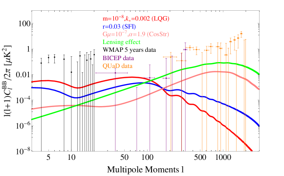
In Fig. 1, we plot the current constraints on the -mode power spectrum along with some representative -mode signals from different theories. The red curve is the predicted calculated from LQG, with a mass parameter and (see Section IV.1 for a discussion on LQG). The blue curve is the predicted from SFI for a tensor-to-scalar ratio , and the pink curve is the BB power spectrum generated by cosmic strings for a string tension and wiggling parameter (see Section V for a discussion on cosmic strings). The green curve is the -mode signal from gravitational lensing which acts as a source of confusion when attempting to measure the primordial -mode signal. The black, purple and orange points with associated error-bars are the currently available -mode data from the WMAP 5-year observations ( lambdaweb ), the BICEP experiment (9 band powers bicepweb ; bicep ), and the QUaD experiment (23 band powers quadweb ; quad ).
The WMAP constraints are relatively weak due to instrumental noise, cosmic variance and residual foreground noise. In addition, the constraining power is further restricted by the uncertainty in the optical depth to the last scattering surface. We will therefore not use the WMAP data in the following likelihood analysis. The BICEP data probes intermediate scales () around the recombination bump in the primordial -mode spectrum. On these scales, the primordial signal is less affected by cosmic variance and is comparable to or larger than the lensing signal for tensor-to-scalar ratios . The QUaD experiment, whose primary aim was a high resolution measurement of the -mode signal, probes small scales (). Its ability to constrain the primordial signal is thus severely restricted due to lensing confusion and the rapid decline in the primordial signal with inverse scale. It may however be useful for constraining the cosmic string signal which peaks on small scales.
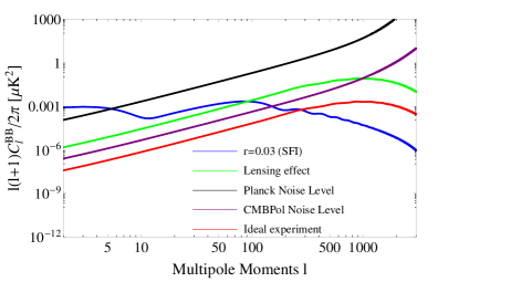
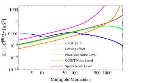
The constraints plotted in Fig. 1 are all consistent with zero signal at the level. Detecting -mode polarization therefore remains an outstanding experimental challenge, and represents a key goal for current and future CMB experiments including ground-based (BICEP-II bicep2 , QUIJOTE quijote , PolarBear polarbear , QUIET quiet ), balloon-borne (EBEX ebex , Spider spider , PIPER) and satellite (Planck planck , B-Pol bpol , litebird litebird , CMBPol cmbpol ) experiments. In what follows, we will forecast the constraints potentially achievable with the following five representative experiments: the Planck and CMBPol satellite missions, the ground-based PolarBear and QUIET (Phase II) experiments, and the balloon-borne experiment, Spider. In addition, for reference, we shall consider the ideal (but unrealistic) case where there is no foreground contamination and no instrumental noise, and where the lensing signal can be cleaned to around 1 part in 40 seljak . The instrumental specifications which we use to model the various experiments are listed in Appendix A. Fig. 2 shows the noise levels of these experiments compared to the SFI signal for .
II.3 Data Analysis Methodology
In this subsection, we describe the methodology we use to constrain the models using current data, and to forecast constraints for future experiments. The parameters of the standard CDM model have already been tightly constrained by CMB TT, EE and TE data Komatsu10 and the remaining uncertainties in these parameters have little impact on the -mode power spectrum, e.g. Lewis06 . Therefore, consistent with the approach adopted by Ref. bicep , throughout this paper, we only vary those parameters which influence the level of primordial -modes. We fix the other cosmological parameters at their WMAP 7-year best-fit values, which are derived under the assumption and constant across all wavelengths Komatsu10 : , , , (pivot scale ), , and .
II.3.1 analysis and hyper-parameters
To constrain the three models using current data, we initially employ a conventional analysis to obtain the likelihood function for each data set. For LQG and SFI, we use the CAMB code CAMBweb to output the transfer function for the -mode power spectrum. can then be calculated as
| (6) |
where is the transfer function for each multipole , and is the primordial tensor power spectrum (see Eqs. (17) and (37)). For the cosmic string model, we use the publicly available code CMBACT CMBACT to generate the -mode power spectrum.
We then follow the pipelines in Refs. bicep ; quad to construct the expected bandpowers for each model, and we use the lognormal approximation (as illustrated in e.g. bicep ) to calculate according to
| (7) |
where is the parameter we wish to constrain, and and are the model and observed band powers, transformed to the lognormal basis. is the covariance matrix of the observed bandpowers, once again transformed to the lognormal basis. Minimizing the across all sampled values of yields the best-fit model.
To obtain joint constraints from BICEP and QUaD, we can simply add the values and minimize the resulting joint ,
| (8) |
The goodness of fit for each model can be ascertained by comparing the minimum value with the number of degrees of freedom . If the value of is close to unity within the range (,), we can say that the model provides a good fit to the data. If , then the model is not a good fit to the data, while if , then the model is overfitting the data which may happen if the model has redundant free parameters and/or the errors on the data have been overestimated.
Note that in the conventional joint analysis of Eq. (8), we have weighted each data set equally. This may be problematic if the two data sets are not mutually consistent, or if there are unquantified systematics in the data Lahav99 ; Hobson02 . In such cases, one may wish to weight the data appropriately. The assignment of weights often occurs when two or more of the data sets are inconsistent, and is usually made in a somewhat ad-hoc manner Hobson02 . Generally speaking, assigning the weights for each data set is a somewhat subjective way of performing a joint analysis, but one well-motivated approach to assigning weights is the “hyper-parameter” approach, formulated within a Bayesian context, which can objectively allow the statistical properties of each data set to determine its own weight in the analysis Lahav99 ; Hobson02 .
In the hyper-parameter technique, the effective is defined as
| (9) |
where sums over all of the data sets, is the for each data set, and is the number of degrees of freedom for each data set 333There is a subtle difference between our definition and those in Lahav99 and Hobson02 . In Lahav99 , is the number of data points in each data set , while in Hobson02 , . However, we prove in Appendix B that, when considering several constraint equations on the random variables, only if the hyper-parameter is defined as Eq. (9), the distribution function form is not changed under the constraints..
Once the values for the combined data set have been obtained, we can find the posterior distribution for the parameter using
| (10) |
where can be either the conventional or the hyper-parameter version Lahav99 .
In Appendix B, we calculate the expectation value and variance (see Eq. (63)) of . This calculation shows that in the hyper-parameter case, a model can be said to be a good fit to the data if the minimum is within the range , where is the number of degrees of freedom for the data sets 444The Bayesian Evidence (BE) is another important technique for discriminating between different models. However, the currently available data is clearly not constraining enough at present to discriminate between models. We therefore defer any discussion of the BE until more precise data becomes available..
II.3.2 Fisher information matrix
In order to make forecasts for the constraints achievable with future experiments, one can make use of the Fisher information matrix under the assumption that each parameter is Gaussian-distributed. The standard Fisher matrix is defined as Kendallbook ; Tegmark97 ,
| (11) |
where is the total covariance matrix, which includes both signal and noise contributions:
| (12) |
Here, is the total noise contribution to the covariance matrix, which includes instrumental noise, foreground contamination as an effective noise, and confusion noise from lensing -modes (see Appendix A for the details). In our case where we consider only -mode polarization, the Fisher matrix can be simplified as Tegmark97 ; fisher2
| (13) |
where is the fraction of sky observed. For Planck, CMBPol, Spider and the ideal experiment, since these are nearly full-sky observations, we perform the summation in Eq. (13) from to . For the ground-based PolarBear and QUIET experiments, the summation is performed from to . We restrict the summation for these experiments to since ground-based experiments are insensitive to the largest angular scales because of their finite survey areas (see jaffe for instance).
The inverse of the Fisher matrix can, crudely speaking, be considered the best achievable covariance matrix for the parameters given the experimental specification. The Cramer-Rao inequality means that no unbiased method can measure the parameter with an uncertainty (standard deviation) less than Kendallbook ; Tegmark97 . If the other parameters are not known but are also estimated from the data, the minimum standard deviation rises to Kendallbook ; Tegmark97 . Therefore we can estimate the best prospective signal-to-noise ratio as , where . This formula will be used frequently in the following discussion.
III Constraining the SFI model
III.1 Scalar and tensor primordial power spectra in the SFI model
In addition to nearly scale-invariant scalar perturbations, inflationary models also predict vector and tensor perturbations grishchuk . However, the vector perturbations are expected to be negligible since these modes decayed very rapidly once they entered the Hubble horizon. We will therefore ignore any vector component in what follows.
We will work in the perturbed Friedmann-Lemaitre-Robertson-Walker Universe, for which the metric can be written as
| (14) |
The tensor perturbations are described by two transverse-traceless components. The power spectrum for the two polarization modes of (, ) is
| (15) |
where is the Fourier component of the perturbation field . Standard inflationary models predict a nearly scale-invariant tensor power spectrum . In order to describe the weak scale-dependence of , we can define the tensor spectral index in the usual way:
| (16) |
The tensor power spectrum can then be written in the following power-law form
| (17) |
In the case where inflation is driven by a single inflaton field, the following calculation yields the primordial power spectrum of the scalar perturbations for slow-roll inflation (see Riotto02 ; Baumann08 for instance. For alternative calculations, see grishchuk2007 .)
| (18) | |||||
while the power spectrum of tensor perturbations is given by
| (19) | |||||
Here, is the inflaton potential, and is the Hubble parameter at the time of inflation. It is customary to define the tensor-to-scalar ratio as
| (20) |
The tensor-to-scalar ratio and the tensor spectral index are related to the slow-roll parameter via Riotto02 ; Baumann08
| (21) |
These expressions lead to the so-called consistency relation for single field slow-roll inflation consistency :
| (22) |
Unfortunately, this consistency relation is extremely difficult to constrain observationally because of the small amplitude of the tensor power spectrum. We discuss the possibilities for testing this relation with future observations in Section III.3.
The normalization of the power spectrum of scalar perturbations (defined at the pivot wavenumber Mpc-1) is ( CL, WMAP 7-year data Komatsu10 ). We can use this normalization together with Eq. (18) to derive the relationship between the energy scale of inflation and the value of :
| (23) |
That is, a detection of the tensor-to-scalar ratio at or greater would indicate that inflation happened at an energy scale comparable to the Grand Unification Theory (GUT) energy scale.
We can also use the slow-roll approximation to derive the following relation, which characterizes the distance in the field space from the end of inflation to the time when CMB scale fluctuations were created, namely the Lyth bound Lyth97 ; Efstathiou05
| (24) |
Thus, a tensor-to-scalar ratio greater than , would directly indicate a super-Planckian field evolving from to . Such a detection could provide important observational clues about the nature of quantum gravity. The boundary is therefore an important benchmark which can confirm or rule out a wide class of large field inflation models.
III.2 Constraints on SFI from current data
In this subsection, we present constraints on the tensor-to-scalar ratio from BICEP and QUaD data. To obtain the constraints, we follow the methodology outlined in Section II.3.1.
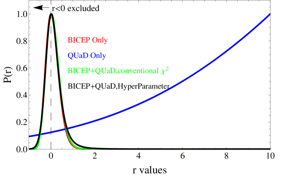
The results of the analysis are shown in Fig. 3. It is clear from the figure that the BICEP data provides a fairly strong upper limit on the value of . The best-fit value is ( CL), which is very close to the result obtained by the BICEP team themselves bicep . As expected, is essentially unconstrained by QUaD, whose measurements are made at much smaller scales () than the scale at which the primordial -mode signal peaks (). In producing joint constraints, we find that both the conventional and the hyper-parameter version () are completely dominated by the BICEP data. For the conventional analysis, the best-fit of the joint analysis gives ( CL), and for the hyper-parameter analysis, we obtain ( CL). The details of the constraints are listed in the first row of Table 1. Note that the tendency for the QUaD data to prefer larger values of appears to be related to a marginal excess of power in the QUaD measurements over the multipole range (see Fig. 1). However, the shape of this apparent “signal” is inconsistent with the SFI model (and indeed with any other primordial -mode model) which suggests that it is likely due to unquantified residual systematics in the data rather than due to a true cosmological signal.
Comparing the BICEP result to the WMAP 7-year results Komatsu10 , the tightest upper-bound on that the WMAP team quote is (). This constraint is derived from a combination of the WMAP data with both large scale structure measurements and the HST key project constraint on the Hubble constant. It is clear that measurements of the and CMB spectra in combination with other astrophysical probes currently play a significant role in constraining the value of . However, we note that the constraints obtained from -mode polarization alone are already comparable to the combined constraints from all other cosmological probes and are likely to overtake them with the next generation of CMB polarization experiments.
In Table 2 we quote the goodness-of-fits for the various analyses and we quote the weights for the hyper-parameter analysis in Table 3. In Table 2, is the expectation value for each fit, calculated using Eqs. (50) and (63). If the model provides a good fit to the data, the minimum over the expectation value should be well within the range (, ). Examining the table, we see that the SFI model can fit the BICEP data well, but that the fit to the QUaD data is relatively poor. This poor fit to the QUaD data adds further weight to our conclusion above regarding the anomalous power in the QUaD results in the range .
| Models | Sampling | Conventional | hyper-parameter | ||
| Range | BICEP | QUaD (tot) | BICEP+QUaD | BICEP+QUaD | |
| SFI: | |||||
| LQG: [Mpl] | |||||
| [Mpc-1] | |||||
| Cosmic String | tot: | ||||
| (l500): | |||||
| Goodness | Conventional | hyper-parameter | ||
| of fits | BICEP | QUaD (tot) | BICEP+QUaD | BICEP+QUaD |
| SFI: | 8 | 22 | 31 | 82.58 |
| 1.00 | 1.64 | 1.56 | 1.26 | |
| Good-fits range | (0.5,1.5) | (0.70,1.30) | (0.75,1.25) | (0.89,1.11) |
| LQG: | 7 | 21 | 30 | 75.49 |
| 1.10 | 1.76 | 1.60 | 1.22 | |
| Good-fits range | (0.47,1.54) | (0.69,1.31) | (0.74,1.26) | (0.90,1.10) |
| CosStr: | 8 | 18 (500) | 27 (QUaD 500) | 66.6 (QUaD 500) |
| 1.0 | 1.35 | 1.21 | 1.08 | |
| Good-fits range | (0.5,1.5) | (0.67,1.33) | (0.73,1.27) | (0.90,1.11) |
| BICEP | QUaD | |
|---|---|---|
| SFI | 1.13 | 0.64 |
| LQG | 1.17 | 0.62 |
| CosStr | 1.13 | 0.95 |
III.3 Prospects for future observations
In this section, we discuss the detection capabilities of future CMB experiments. In order to forecast the error bars of the parameters and in the fiducial models, we use the Fisher matrix technique, introduced in Section II.3.2.
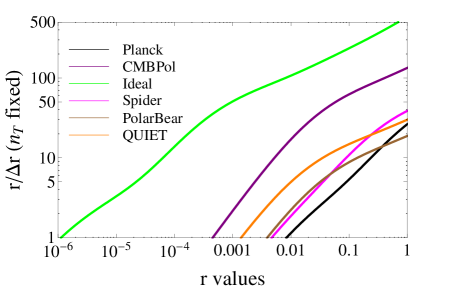
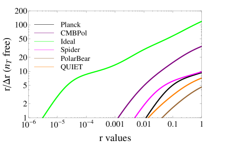
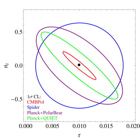
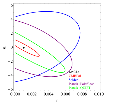
In Fig. 4, we plot the signal-to-noise ratio () for a detection of tensors as a function of the fiducial value of , for a number of current and forthcoming experiments. In the left panel, we only consider as the free parameter, and keep fixed at . We see that the Planck satellite can potentially detect the signal of the tensor perturbations at more than confidence level if . For , the value of becomes which would constitute a robust detection. These results are consistent with those presented in Efstathiou09 ; zbg2010 . The predicted constraints for PolarBear, QUIET and Spider are somewhat tighter with for models with . The predicted constraints for the proposed CMBPol mission suggest that tensor perturbations could be detected (at the 3 level) for values of as low as . Such a measurement would provide an excellent opportunity to differentiate between various inflationary models. We also find that for the ideal CMB experiment which includes only a residual lensing noise contribution (after de-lensing), the SFI primordial signal could be detected (at ) only if is satisfied.
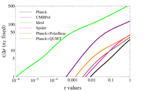
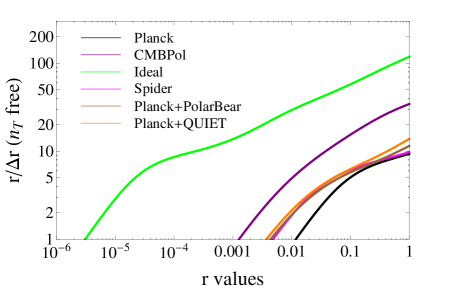
In Fig. 5, we also plot the signal-to-noise ratio for the combination of Planck with the ground-based experiments (PolarBear and QUIET). The former is sensitive to the -mode signal at the lowest multipoles , while the latter are sensitive to the recombination peak of at . Similar to zb , we find that the combination of these experiments yields little formal improvement in the signal-to-noise of the detection compared with the capabilities of the ground-based experiments on their own. However, a detection of both the recombination bump (e.g. from ground-based experiments) and the reionization bump (e.g. from Planck) would constitute much more compelling evidence for tensors than either detection would constitute on its own.
In the right hand panels of Fig. 4 and Fig. 5, we have plotted the results for the case where we treat both and as free parameters. Comparing with the corresponding results in the left panels, we find (in agreement with previous works, e.g. cmbpol ; nt2 ) that the signal-to-noise ratios become much smaller due to correlations between the parameters. These correlations were investigated in some detail by zb who also explored the optimal choice of pivot scale for which the two parameters become decorrelated.
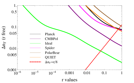
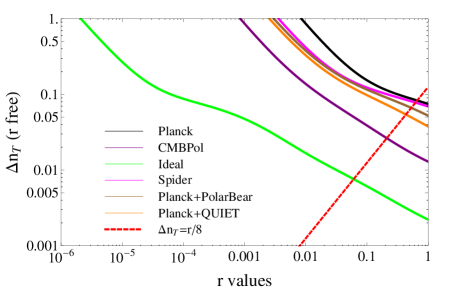
In Fig. 7, we plot the values of as a function of for various cases. Here we find that, for Planck, PolarBear, QUIET and Spider, the constraint on is relatively weak unless the value of is very large. For example, the predicted constraint for Planck is , and for QUIET is for a model with . The combination of Planck and QUIET could in principle do somewhat better with . The proposed CMBPol mission could achieve while the limiting value of the ideal experiment is , which is comparable to the current constraint on the scalar spectral index Komatsu10 . For lower values of , the predicted constraints are correspondingly weaker. For example, for the CMBPol mission, the value of increases from to if we replace the model with .
Testing the consistency relation (see Eq. (22)) is potentially one of the most powerful ways to test the general SFI scenario. To assess whether future experiments might achieve this goal, in Fig. 7 we compare the values of with . If , then the constraint on is tight enough to allow the consistency relation to be tested. We find that is satisfied only if for the CMBPol experiment, and only if for the ideal experiment. An observational confirmation of the consistency relation is therefore extremely unlikely to be achieved with any of the currently envisaged future experiments.
III.4 Single-field slow-roll inflationary models
In this subsection, we discuss four types of single field slow-roll inflationary models, categorized by cata , and the implications for these models of the results presented in the previous section.
In single field slow-roll inflationary models, the observables depend on three slow-roll parameters slow-roll
| (25) |
where is the inflationary potential, and the prime denotes derivatives with respect to the field . Here, quantifies the “steepness” of the slope of the potential, measures the “curvature” of the potential, and quantifies the “jerk”. Since the potential is fairly flat in the slow-roll inflation models, these three parameters must be much smaller than unity for inflation to occur. One of the important predictions of SFI models is that the scalar perturbations are nearly scale-invariant, which has already been confirmed by WMAP results Komatsu10 .
In SFI models, a standard slow-roll analysis yields the following relations
| (26) |
where is the tilt of primordial scalar power spectrum, and is the “running” of . These formulae relate the tensor parameters and to the scalar parameters and ; the latter can be constrained through CMB and large scale structure observations. As shown in Eq. (26), the relation between and involves the slow-roll parameter which in turn depends on the specific inflationary potential.
The strength of the primordial tensor perturbations depends on the value of . Observations have yielded quite tight constraints on , but we currently only have upper limits on the value of . The relation between and depends on the specific inflationary model, and different models predict very different values for . In the following discussion, we categorize SFI models into four classes based on different regimes for the curvature of the potential , and discuss their individual constraints.
Case A: negative curvature models
The negative models arise from a potential of spontaneous symmetry breaking. One type of often-discussed potentials is the form (). This type of model predicts a red tilt in the scalar spectrum (), which is consistent with the WMAP 7-year results Komatsu10 . In addition, these models predict relatively small values for . For the model with in Ref. cata ,
| (27) |
where is the number of e-folds, taken to be in the range based on current observations of the CMB N ; Komatsu10 . Here we choose the value . Using the result Komatsu10 yields the constraint . From Fig. 4 (right panel), we see that this is close to or even beyond the sensitivity range of the Planck satellite, but is within the sensitivity ranges of PolarBear, QUIET, Spider and CMBPol. In other models with , the predicted values of are much smaller than that of the model with .
Case B: small positive curvature models
Two example potentials in this case are the monomial potentials with for and the exponential potential for . In these models, to first order in slow roll, the scalar index is always red and the following constraint on is satisfied
| (28) |
Using the result Komatsu10 , one finds that , which is within the sensitivity range of the Planck satellite, as well as that of forthcoming CMB experiments. Thus, the Planck results may provide some constraints on these type of models.
Case C: intermediate positive curvature models
The supergravity-motivated hybrid models have a potential of the form , up to one-loop correction during inflation. In this case,
| (29) |
are satisfied. Using the result Komatsu10 , one finds that , which is slightly in conflict with the current upper limit (WMAP+BAO+, CL) Komatsu10 . Fig. 4 shows that this model is also in the sensitivity range of the Planck satellite.
Case D: large positive curvature models
This class of models has a typical monomial potential similar to those of Case A, but with a plus sign for the term : . This enables inflation to occur for small values of . The model predicts a blue tilt in the scalar power spectrum (Eq. (26)), which is in conflict with current constraints on unless a running of is allowed Komatsu10 . When a running in is included, the WMAP 7-year results suggest a blue power spectrum ( for CL). Therefore, even though this model is not favoured by the WMAP 7-year results for the case of constant , it is not excluded when a running of the spectral index is included. Planck and future CMB experiments should constrain both and to high precision and so should be able to definitively rule out this model.
IV Loop Quantum Gravity and its observational probes
IV.1 Primordial tensor perturbations in LQG models
Loop Quantum Gravity is a promising framework for constructing a quantum theory of gravity in theoretical physics. Based on the reformulation of General Relativity as a kind of gauge theory obtained by Sen81 ; Ashtekar96 , LQG is now a language and a dynamical framework which leads to a mathematically coherent description of the physics of quantum spacetime Grain09 . Constraining LQG theories experimentally is challenging because the quantum geometrical effect can only be tested at very high energy scales, beyond the reach of current accelerator experiments. In this section, we will calculate the possible observational signature of LQG in the CMB sky, which opens a new window for cosmological tests of quantum gravity.
There are two main quantum corrections in the Hamiltonian of LQG when dealing with the semi-classical approach, namely holonomy corrections and “inverse volume” corrections Grain09 ; Mielczarek10 . The holonomy corrections lead to a dramatic modification of the Friedmann equation as Singh06
| (30) |
where is the energy density, and is the critical energy density,
| (31) |
Here is the Barbero-Immirzi parameter, which is derived from the computation of the black hole entropy Meissner04 . Note that we use the reduced Planck mass in our calculation.
A generic picture for this model with the holonomy correction is the bouncing behavior exhibited when the energy density of the Universe approaches . The negative sign in Eq. (30) is an appealing feature in the framework of LQG such that the repulsive quantum geometry effect becomes dominant in the Planck region Grain09 ; Mielczarek10 . This triggers a contraction period before the bounce, during which time the Hubble parameter is negative and the Hubble radius is shrinking. As a result, the perturbation modes on the largest scales crossed the Hubble horizon and froze out during the contracting period, until the end of the contracting stage when the Hubble horizon increased again. For the very large scale modes, this pre-inflationary bounce may imprint distinctive features in the CMB sky, since they stretched out of the horizon at very early times Grain09 ; Mielczarek10 .
Unfortunately, the power spectrum for the scalar perturbations is somewhat hard to obtain because in the case of the holonomy correction, the anomaly free equations are still to be found Mielczarek10b . Therefore, in the following discussion, we will focus on the tensor power spectrum of LQG and pursue the constraints obtainable on the model from -mode observations.
Due to the pre-inflationary contracting period, the tensor power spectrum for LQG can be calculated numerically. In Mielczarek10 , a simple parameterized form of the power spectrum is introduced as follows
| (32) |
where is the Hubble parameter during the inflationary stage, is the position of the highest peak in the power spectrum, and the quantity is related to the mass of the scalar field as
| (33) |
It is interesting to note that Eq. (32) reduces to the SFI result of Eq. (19) for . In this paper, for simplicity, we consider the tensor power spectrum (Eq. 32) with a constant in the early stage of inflation, which corresponds to the specific case of de Sitter inflation.
In this model, we assume that inflation is driven by the potential . The Hubble parameter is related to this potential via
| (34) |
where is the initial value of the scalar field at the beginning of inflation. The number of e-folds can be calculated as (using the slow-roll approximation )
| (35) | |||||
Since , the above equation is approximately given by The Hubble parameter is then (from Eq. (34))
| (36) |
Substituting this into Eq. (32), we arrive at the following expression for the tensor power spectrum:
| (37) |
where is the number of e-folds which we fix at . Finally, we use Eq. (6) to project the perturbation modes onto the CMB sphere to find for the LQG model.
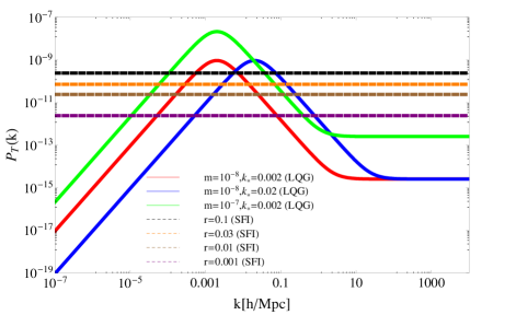
In the left panel of Fig. 8, for a number of representative sets of parameters, we plot the primordial tensor power spectrum for the LQG model alongside the signal expected in an SFI model for a number of different values of . For the SFI model, since the power spectrum tilt is very small ( for de Sitter inflation), the power spectrum is very flat on all scales. In comparison, the tensor power spectrum of LQG exhibits a bump feature, which is in fact the signature of the pre-inflationary contraction period. Very large scale modes stretched out of the Hubble horizon during the contracting period before inflation, and can be described by the solution in the Minkowski vacuum Grain09 ; Mielczarek10 . Thus, the power spectrum at very large scale takes the form Grain09 ; Mielczarek10 . In contrast, the small scale modes are well within the Hubble horizon and so the power on small scales is similar to the scale-invariant power spectrum of the SFI model. The bump in the power spectrum on larger scales is characterized by the magnitude of . As increases, the bump is shifted to smaller scales and vice versa. The amplitude of the spectrum and the width of the bump are determined by the mass parameter . We will link these two important parameters to the energy scale of inflation and the current Hubble horizon scale in the next subsection.
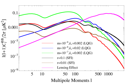
The right panel of Fig. 8 shows that the bump in the primordial power spectrum results in a peak in the CMB -mode power spectrum, which is slightly different to that of the SFI model. In addition, if the peak of the LQG spectrum is normalized to the same magnitude as that of SFI, the small scale power will be suppressed in the LQG model, as compared to the SFI model.
IV.2 Constraints from current data
In this subsection, we use the BICEP and QUaD data to constrain the parameters of LQG models. Before we perform the parameter estimation, we link the two parameters and with the energy scale of inflation, and with the current Hubble horizon scale.
The parameter relates to the energy scale of inflation in LQG as follows
| (38) |
where is around the GUT energy scale. Therefore, a detection of would strongly suggest that the energy scale of inflation is above the GUT scale.
The parameter describes the position of the peak in the primordial power spectrum. We can compare it with the current Hubble wavenumber, which is . If , then modes with physical wavelengths () equal to the Hubble horizon at the beginning of inflation will have wavelengths less than the current Hubble horizon, whereas if their wavelengths will be larger than the current horizon scale. Thus, if , we would expect to be able to find pre-inflationary fluctuations within our current Hubble horizon Grain09 ; Mielczarek10 . Conversely, as , the primordial tensor power spectrum (Eqs. (32) and (37)) reduces to the scale-invariant tensor power spectrum as noted above. Therefore, a non-zero detection of would strongly indicate the existence of a bounce and of a contracting period before inflation.
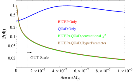
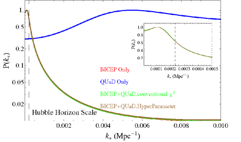
The current constraints on the parameters and are shown in Fig. 9. In the left panel, we have marginalized over the parameter and we plot the PDF for the mass parameter . The upper bound is . The detailed results are listed in the second and third rows of Table 1. We note that the GUT scale mass is excluded at the level, but is still well within . As was the case with the SFI models, the small-scale QUaD data is unable to constrain the LQG models. Once again, the combined constraints are dominated by the BICEP data as is clear from the figure and from the results listed in Table 1.
In the right panel of Fig. 9, we show the PDF for (marginalized over the parameter). Once again the results are dominated by BICEP. From this plot, wee see that there is a peak in the PDF at . Although it is not statistically significant, a detection of such a feature would be an interesting result for the pre-inflationary bouncing behavior, since the bounce of the primordial tensor power spectrum is characterized by a non-zero as we have already discussed. We further note that the peak value of is only slightly smaller than the current Hubble wavenumber , which would indicate that modes which had the same length scale as the Hubble horizon at the beginning of inflation have not evolved into the Hubble horizon yet. In that case, the bump in the tensor power spectrum of LQG is a super-horizon feature. However, we stress again that all of our results are upper limits only and our formal constraint is ( CL).
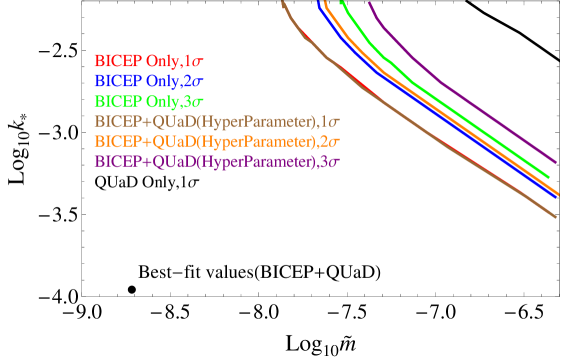
In Fig. 10, we plot the two-dimensional constraints on the parameters and on a log scale. Clearly, the current data is unable to provide strong constraints on the joint distribution of these two parameters and can only provide upper limits. Once again, as expected, the constraints are dominated by the BICEP data.
IV.3 Prospects for future experiments
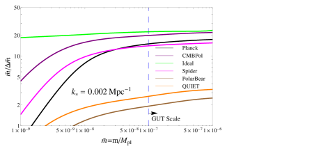
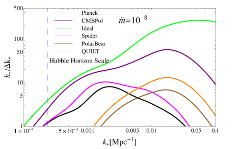
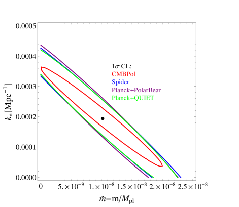
We now investigate the prospects for detection of LQG signatures with future CMB experiments by studying the projected constraints on the two parameters and . Once again, we use the Fisher matrix approach described in Section II.3.2 and as in Section III.3, we fix the background parameters at their WMAP 7-year best-fit values Komatsu10 .
In Fig. 11, we plot the projected signal-to-noise ratio for the parameters (left panel) and (right panel) for forthcoming experiments. In the left panel, we plot the signal-to-noise ratio as a function of . For this plot, we have kept fixed at Mpc-1. We find that, if Mpl, i.e. the energy scale of inflation is higher than the GUT scale, then Planck, Spider and CMBPol could potentially detect the LQG signal at more than due to their large sky coverage. In contrast, the smaller scale experiments (PolarBear and QUIET) would only detect the signal at the 2—3 level. For Mpl, close to the upper bound of the current confidence level, the large scale survey experiments (Planck, Spider and CMBPol) can still detect the signal at more than . For this mass parameter and value of , the ground-based experiments, PolarBear and QUIET, would be insensitive to the signal since the -mode power spectrum from LQG falls off extremely rapidly with increasing . However, for larger values of , the peak of the LQG power spectrum moves to smaller scales. We therefore expect a general trend whereby the large-scale experiments will be sensitive to models with small values of and small-scale experiments will be sensitive to models with larger values of .
This is illustrated in the right-hand panel of Fig. 11 where we plot forecasts for as a function of . For these results, we have fixed Mpl. We find that the signal-to-noise ratio of does not monotonically increase with increasing for any single experiment. Since this parameter controls the angular scale at which the LQG -mode signal peaks, as we vary we move between the sensitivity ranges of different experiments. For example at Mpc-1, both Planck and Spider could detect the signal at more than whereas PolarBear and QUIET would achieve only a marginal detection. Conversely, if Mpc-1, the reverse is true: PolarBear and QUIET would make strong () detections while Planck and Spider would struggle to detect a signal.
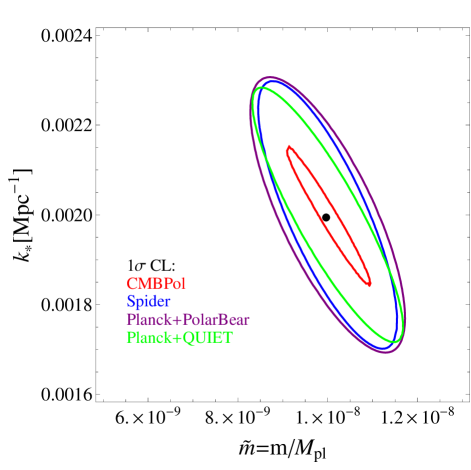
In Fig. 12, we plot the two-dimensional constraints on the parameters and for two typical models. The left panel shows the forecasted constraints for a model with Mpc-1 and the right panel shows the constraints for a model with Mpc-1. In both cases, a fiducial value of Mpl was adopted. We find that the former case can be well constrained by either Spider, CMBPol, Planck+PolarBear or Planck+QUIET while the latter case can only be meaningfully constrained by the CMBPol mission.
V Cosmic strings and their detection
V.1 -mode polarization from cosmic strings
Cosmic strings have been proposed as a possible source of the inhomogeneities in the Universe cosmicstring . Although current observations of the CMB temperature and polarization power spectra suggest that it is inflation, rather than cosmic strings, which is the main source of the primordial density perturbations Komatsu10 , there is still significant motivation to search for the signature of cosmic strings from both theoretical and observational considerations.
Cosmic strings can be formed in several inflationary pictures, and particularly in Brane inflation models kklt ; Kachru03 ; braneinflation . Brane inflation arises from the framework of high dimensional string theory and is a further important model for sourcing the dynamics of inflation. In this model, the high dimensional Brane and anti-Brane collided and annihilated and cosmic strings were produced at the end of the inflationary epoch. If this scenario is correct, the resulting strings would have made an observable imprint on the CMB sky by way of the Kaiser-Stebbins effect kseffect .
Although current observations suggest that inflation sources the majority of the CMB anisotropy, one cannot rule out a significant (up to ) contribution from cosmic strings stringconstraint . In this section, we will use CMB data to constrain the level of cosmic strings. However, in contrast to other works (see e.g. stringconstraint ), we focus on the possible detection of cosmic strings through the -mode power spectrum alone. -mode polarization can only be generated in the early Universe by vector and tensor perturbations, which provides a complementary route for detecting cosmic strings. Although the contribution of scalar perturbations from cosmic strings is subdominant () compared to the contribution from SFI, the contributions of vector and tensor perturbations from cosmic strings may constitute a very significant fraction of the -mode polarization power on small angular scale (high multipoles) Pogosian08 .
To predict the power spectrum generated by cosmic strings, one must understand the evolution of a cosmic string network and it is important to know the characteristics of the scaling regime which needs to be assumed in the numerical simulation. There are two popular ways of making progress. One is to solve the Nambu equations of motion for a string in an expanding universe and ignore the effects of radiation backreaction (hereafter the Nambu-String model); the other is to solve the equations of motion for the Abelian-Higgs (AH) model, but to limit the dynamical range of the simulation. In this work, we will consider only the Nambu-String model but we note that the Abelian-Higgs model can be constrained in a similar way.
In order to calculate the -mode power spectrum, including the contributions of both vector and tensor perturbations, we use the publicly available code CMBACT CMBACT ; Pogosian99 to generate a fiducial for cosmic strings with the tension of the strings set to . Since the amplitude of the -mode power spectrum generated by cosmic strings is simply proportional to the square of the cosmic string tension, we can scale the fiducial spectrum to any other value for the cosmic string tension using
| (39) |
where is the power spectrum normalized at .
V.2 Constraints from current data
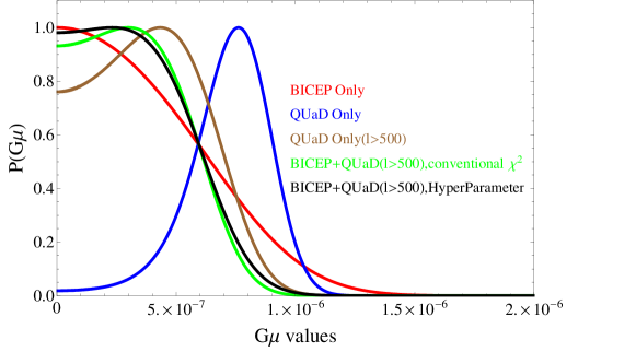
In Fig. 13, we show the current constraints on the cosmic string tension from the BICEP and QUaD data. The upper bound from BICEP alone is ( CL). Using the QUaD data alone the result is , shown as the blue curve in Fig. 13. Taken at face value, the QUaD result represents a detection of the cosmic string tension. Referring back to Fig. 1 and the discussion in Section III.2, this result is likely coming from the apparent excess of power seen in the QUaD data on scales . To investigate further, we have repeated the analysis with the QUaD data removed. This results in the likelihood function for shown as the brown curve in Fig. 13. Excluding the QUaD data shifts the peak of the likelihood significantly towards a smaller value (best-fit ), and the constraint is now consistent with zero at the CL. The upper limit becomes (see Table 1 for the full set of results). The fact that the QUaD result changes drastically when we remove the measurements suggests a problem with the data. As in the case of the SFI constraints presented earlier, we note that the shape of the QUaD data at is clearly inconsistent with the expected -mode signal for cosmic strings. Once again, we suspect that the anomalous signal seen in the QUaD data between and is likely due to unquantified systematics. We therefore consider the QUaD result restricted to to be a more robust constraint and consequently we quote this as our main result.
We now examine the constraints obtained from combining the BICEP data with the QUaD data. Since the peaks of the two likelihood functions do not overlap, we will carefully consider both the conventional analysis and the hyper-parameter . When we use the conventional , the peak of the combined likelihood lies midway between the peaks of the two individual likelihoods (green line in Fig. 13), and the resulting constraint is ( CL). If we use the hyper-parameter , the peak of the joint distribution moves slightly further towards zero, and the best-fit is ( CL). Since the conventional and hyper-parameter approaches give very similar results, this suggests that the BICEP and QUaD data are mutually consistent which adds confidence to the joint constraint.
A number of previous works have also attempted to constrain cosmic strings through their imprint on CMB (), large scale structure and gravitational waves data constrain-bbn ; constrain-pulsar ; constrain-ligo ; constrain-cs1 ; constrain-cs2 ; constrain-cs3 . In a recent work stringconstraint , constraints on the cosmic string tension were obtained from a combination of CMB data (including the WMAP 5-year, ACBAR, BOOMERGANG, CBI, QUAD and BIMA observations), matter power spectrum data from the SDSS Luminous Red Galaxies sample, and Big Bang Nucleosynthesis constraints on the baryon fraction from measurements of deuterium at high redshift. They obtained a combined upper limit of () in the Nambu-String case.
As expected, this limit is much tighter than what we have obtained from -modes alone since current measurements of the and power spectra are much stronger than the data that we have used here. However, we note that in the analysis of Ref. stringconstraint , the main constraining power comes from the CMB and SDSS data and ultimately constraints from such data will be limited by degeneracies with other parameters (most notably, the spectral index ). As is the case for SFI models, the advantage of using the power spectrum to constrain the cosmic string tension is that is only very weakly dependent on the other cosmological parameters, e.g. . Our constraint is therefore an independent check of other constraints obtained on using different data and our result, although weaker, is consistent with previous analyses. Cosmic string constraints from forthcoming CMB polarization experiments will likely close the gap with other techniques in terms of constraining power. We now turn to examining the constraints achievable with these forthcoming experiments.
V.3 Prospects for future experiments
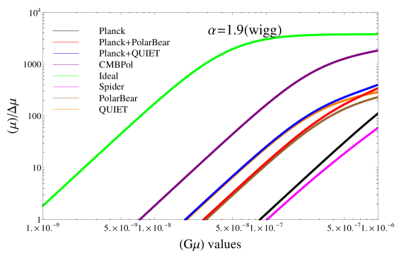
In this subsection, we forecast the detectability of the cosmic string tension for future experiments. Once again, we use the Fisher matrix formalism described in Section II.3.2. In Fig. 14, we plot the signal-to-noise ratio for a measurement of for the various experiments. As one might expect, the Planck and Spider experiments are unable to tightly constrain the cosmic string tension since neither experiment will produce sensitive -mode measurements on small scales where the string signal peaks.
For example, the Planck satellite can detect a cosmic string signal at the level only if is satisfied. The ground-based experiments, PolarBear and QUIET, will obviously be better at constraining than Planck and Spider. PolarBear should be able to detect (at the level) while QUIET should be able to detect (again at ). Adding Planck to either of these experiments does not change the results significantly. CMBPol is much more sensitive than the other experiments for all fiducial values, and its detection limit is . Finally, we find that the ideal CMB experiment can detect cosmic strings at the level if is satisfied, which represents the fundamental detection limit for CMB -mode polarization experiments.
VI Conclusion
In this paper, we have examined the observational signatures of three different models of the early Universe related to the inflationary process. These three models are in turn motivated by three different aspects of microscopic physics: single field slow-roll inflation from effective field theory (SFI), loop quantum cosmology from loop quantum gravity (LQG) and cosmic strings from Brane inflation and/or high dimensional string theory. We have discussed their potential observational signatures in the -mode polarization of the CMB, and we have constrained the parameters of each model using the latest CMB polarization data from the BICEP and QUaD experiments. Using a Fisher matrix formalism we have forecasted the constraints achievable on these models using future CMB polarization observations from a number of experiments including Planck (space), PolarBear (ground), QUIET (ground), Spider (balloon), CMBPol (space) and an idealized experiment.
We first discussed the SFI model. From the Lyth bound relation, we know that is an important bound for inflation reaching the GUT scale, and the inflaton evolves over the trans-Planckian region. The constraints we obtained from current -mode measurements are shown in Fig. 3. Using the BICEP data alone, we find ( CL) in close agreement with the BICEP team’s own analysis bicep . As expected, this constraint does not change significantly on the addition of the small-scale QUaD data. Looking to the future, we find that the Planck satellite may be able to detect (at the CL), while the Spider, QUIET and PolarBear experiments all have the potential to make a detection of . The possible future satellite mission, CMBPol could detect at the CL, and could even detect at the CL. (All of these forecasts are for the case where the tensor spectral index is held fixed at .) In summary, we find that all future experiments can potentially constrain the value of with sufficient sensitivity to allow the SFI model from effective field theory to be tested in an interesting way.
We have also discussed the LQG model, which predicts a pre-inflationary bouncing era. Before the bounce, the Universe was contracting and dominated by vacuum energy. Its tensor power spectrum is characterized by two parameters: and , where the mass parameter controls the magnitude of the -mode power spectrum, and controls the scale of the peak in the -mode spectrum. Our joint likelihood analysis using current data yields and Mpc-1 (both CL upper limits). The PDF for the parameter exhibits a peak at position Mpc-1. Although this peak is not statistically significant, we note that were the value of to be around this value, this would constitute evidence for a pre-inflationary bounce. We have also presented forecasts for constraining the LQG model using future CMB experiments. We find that if the value of is as large as Mpc-1, a number of ongoing and future experiments (Planck, Spider and CMBPol) could potentially detect the signal as long as Mpl. However, if the value of were to be as low as Mpc-1 (as is mildly indicated by current data), then the signature of LQG becomes quite difficult to detect. We find that, for a typical choice of Mpl, only CMBPol and the ideal experiment could detect the signal for such a low value of .
Finally, we have presented current and prospective constraints on the cosmic string tension. We find that the BICEP and QUaD data constrain the cosmic string tension to be and respectively (both CL upper limits). The combined constraint is , which is weaker, but comparable to the constraints from the CMB temperature anisotropy power spectrum. In terms of forecasts for the future, we find that the high-resolution ground-based experiments, PolarBear and QUIET, are more useful for constraining (as compared to e.g. Planck and Spider) since they are much more sensitive to the -mode power spectrum on small angular scales. These two experiments could detect at more than CL. We also find that CMBPol can detect the signal of cosmic strings if at CL, and the ideal CMB experiment can detect the signal at the level even if the tension of cosmic string is as low as .
Although the -mode polarization derived constraints which we have presented in this paper are currently only upper limits, they are nevertheless already comparable to the equivalent constraints obtained using a combination of all other cosmological data. In terms of constraining the parameters of early Universe models, -mode polarization is clearly a very powerful tool and will likely overtake other early Universe probes with the advent of the next generation of CMB polarization experiments. In this paper, we have not directly considered the issue of model selection. However, it is likely that, in addition to constraining model parameters, future sensitive -mode observations will also allow us to distinguish between models of the early Universe such as those considered in this paper.
Acknowledgements.
The authors acknowledge useful communications and discussions with Richard Battye, Daniel Baumann, Cynthia Chiang, Anthony Challinor, George Efstathiou, Eanna Flanagan, Christopher Gordon, Michael Hobson, Deepak Baskaran, Leonid Grishchuk and Mao Zeng. Yin-Zhe Ma thanks Trinity College Cambridge and Cambridge Overseas Trusts for support.Appendix A Instrumental Characteristics of CMB Experiments
| Band center [GHz] | 30 | 44 | 70 | 100 | 143 | 217 | 353 |
|---|---|---|---|---|---|---|---|
| FWHM [arcmin] | 33 | 24 | 14 | ||||
| [K2] | 2683 | 2753 | 2764 | ||||
| Band center [GHz] | 90 | 150 | 220 |
|---|---|---|---|
| FWHM [arcmin] | |||
| [K2] | 5.2 | 4.3 | 44.0 |
| Band center [GHz] | 40 | 90 |
| FWHM [arcmin] | ||
| [K2] | 0.26 | 0.64 |
| Band center [GHz] | 100 | 145 | 225 | 275 |
| FWHM [arcmin] | 26 | 21 | ||
| [K2] | 84.4 | 47.4 | 395 | 1170 |
| Band center [GHz] | 30 | 45 | 70 | 100 | 150 | 220 | 340 |
|---|---|---|---|---|---|---|---|
| FWHM [arcmin] | 26 | 17 | 11 | ||||
| [K2] | 31.21 | 5.79 | 1.48 | 0.89 | 0.83 | 1.95 | 39.46 |
| Parameter | Synchrotron | Dust |
|---|---|---|
| K2 | K2 | |
| 30 GHz | 94 GHz | |
| 350 | 900 | |
| -3 | 2.2 | |
| -2.6 | -1.4 |
To calculate the total noise power spectrum (Section II.3.2), we require the experimental specifications of each experiment, including the levels of both residual foreground noise and instrumental noise. We list the instrumental noise for each frequency channel the experiments we have considered in Table 4-8. The effective noise power spectrum is given by the optimal combination of the channels cmbpol
| (40) |
where and are the instrumental and residual foreground noise power spectra, respectively. Note that the noise power spectra listed in the tables do not include the window function of the instrumental beam .
To model polarized foregrounds, we focus on diffuse synchrotron (S) and dust (D) emission. The foreground contamination can be quantified by the parameter which multiplies the power spectra , of the foreground models. The smaller the value of the deeper the foreground cleaning. Throughout this paper, we adopt . The residual foreground noise is given by (see cmbpol for instance)
| (41) |
where is the noise power spectrum arising from the cleaning procedure itself in the presence of instrumental noise.
Following foreground3 ; cmbpol ; foreground2 , we model the scale () and frequency () dependence of the synchrotron and dust emission as
| (42) |
and
| (43) |
In Eq. (43), is the dust polarization fraction, estimated to be foreground3 , and is the temperature of the dust grains, assumed to be constant across the sky with K foreground3 . Other parameters in Eqs. (42), (43) are specified in Table 9 taken from cmbpol .
The noise term () entering Eq. (41) is calculated in foreground3 ; cmbpol
| (44) |
Here, is the total number of frequency channels used in making the foreground template map, and is the frequency of the reference channel. In the case of dust, is the highest frequency channel included in the template making, while in the case of synchrotron, is the lowest frequency channel. The value of is given in Table 9 for different foreground models. We note that the ground-based experiments are insensitive to the largest angular scales, so when calculating the Fisher matrix using Eq. (13), we sum over the from 21 to 3000. In addition, for ground-based experiments, the small scale fluctuations are not very sensitive to the residual foreground noise, and we can also pick out relatively clean patchs of sky where the foreground contamination is minimal. Therefore, to forecast the results for PolarBear and QUIET, we have not included a residual foreground noise term.
In addition to instrumental and residual foreground noise, gravitational lensing converts -mode polarization into -modes on small angular scales, contaminating the primordial -mode signal lensing . The lensed will also contribute to the total noise power spectrum . The total noise power spectrum therefore becomes
| (45) |
For the ideal case, we assume that there is no instrumental or foreground noise, and that we can successfully de-lens the CMB observations to a level of about of the lensing signal seljak . In this case, the total effective noise power spectrum is
| (46) |
Finally, we adopt for the ideal experiment, which is the same as that used to model CMBPol.
Appendix B Statistics of the conventional and the hyper-parameter
In this appendix, we first review the basic results of conventional statistics and then generalize the analysis to the hyper-parameter technique.
B.1 statistics
A conventional joint analysis will minimize the following combined
| (47) |
where each follows the chi-square distribution
| (48) |
It is easy to show that this chi-square distribution is properly normalized, i.e.
| (49) |
and the expectation value and the variance are
| (50) |
Therefore, the minimum value of a properly constrained model should satisfy the following relation
| (51) |
For the with order , this is
| (52) |
If the , we can say that the model does not provide a good fit to the data, whereas if , we say that the model overfits the data, which may mean that the model has redundant free parameters.
If there are constraints on the random variables, then still follows the chi-square distribution, but with order Rileybook
| (53) |
It is straightforward to verify, that the shape of the distribution does not change, but the expectation value and the variance are changed simply as .
B.2 Hyper-parameter
The hyper-parameter approach to combining the constraints from different data sets can be useful in the case where the different data sets have different levels of systematics. To weight each data set, one should multiply each by a free parameter,
| (54) |
where is the weight parameter for each data set. One can marginalize these weight parameters in a Bayesian analysis, and in Lahav99 , the authors found that instead of minimizing the combined one should instead minimize the following quantity
| (55) |
where is the number of degrees of freedom for each data set. If we only consider one data set, the hyper-parameter statistic becomes
| (56) |
From Eq. (48), using the following transformation
| (57) |
one can show that the distribution of the hyper-parameter statistic is given by
| (58) |
which has already been properly normalized. (When calculating the integral, one should use the transformation ). One can then show that the expectation value and variance of the Hyper-parameter distribution is
| (59) |
where is the “digamma function” defined as derivatives of the log Gamma function
| (60) |
If there are constraints on the random variables (e.g. parameters), then the distribution of the conventional follows Eq. (53). It is then easy to show that the form of the distribution is unchanged only if the is defined as
| (61) |
Proof From Eqs. (53) and (57), one can derive the following PDF
| (62) | |||||
Therefore, in the case of constraints, the distribution keeps its form, and the expectation value and variance become
| (63) |
Thus, to ensure that the form of the distribution function is unchanged, the needs to be defined as
| (64) |
where is the number of degree of freedom.
The hyper-parameter approach is an objective way to weight each data set when producing joint constraints. The value of the weight is simply the value of the effective hyper-parameter, which is defined as Lahav99
| (65) |
where A specifies a particular data set. Therefore, the larger the value of , the larger the weight that the particular data set takes (see Table 3).
References
- (1) C. L. Bennett et al., Astrophys. J. Suppl. 148, 1 (2003).
- (2) G. Hinshaw et al., Astrophys. J. Suppl. 170, 288 (2007).
- (3) E. Komatsu et al., arXiv: 1001.4538.
- (4) A. Lewis and A, Challinor, Phys. Rept. 429 (2006) 1-65.
- (5) M. L. Brown et al., Astrophys. J. 705, 978 (2009).
- (6) H. C. Chiang et al., Astrophys. J. 711, 1123 (2010).
- (7) J. Kovac et al., Nature (London) 420, 772 (2002).
- (8) A. C. S. Readhead et al., Science 306, 836 (2004).
- (9) C. Bischoff et al. (CAPMAP Collaboration), Astrophys. J. 684, 771 (2008).
- (10) W. C. Jones et al., Astrophys. J. 647, 823 (2006).
- (11) J. H. P. Wu et al., Astrophys. J. 665, 55 (2007).
- (12) A. Borde and A. Vilenkin, Phys. Rev. Lett. 72, 3305 (1994).
- (13) V. F. Mukhanov, H. A. Feldman and R. H. Brandenberger, Phys. Rept. 215, 203 (1992); R. H. Brandenberger, Lect. Notes Phys. 646, 127 (2004).
- (14) S. Kachru, R. Kallosh, A. Linde and S. P. Trivedi, Phys. Rev. D 68, 046005 (2003).
- (15) S. Kachru, R. Kallosh, A. Linde, J. M. Maldacena, L. McAllister and S. P. Trivedi, JCAP 0310, 013 (2003); Y. Z. Ma and X. Zhang, JCAP 03, 006 (2009).
- (16) N. T. Jones, H. Stoica and S. H. Tye, JHEP 0207, 051 (2002).
- (17) S. Sarangi and S. H. Tye, Phys. Lett. B 536, 185 (2002).
- (18) M. Bojowald, Living Rev. Relativity, 11, 4 (2008).
- (19) U. Seljak and M. Zaldarriaga, Phys. Rev. Lett. 78, 2054 (1997); M. Kamoinkowski, A. Kosowsky and A. Stebbins, Phys. Rev. Lett. 78, 2058 (1997).
- (20) W. Zhao, D. Baskaran and L. P. Grishchuk, Phys. Rev. D 79, 023002 (2009); 80, 083005 (2009); W. Zhao, Phys. Rev. D 79, 063003 (2009).
- (21) S. Chandrasekhar, in Radiative Transfer (Dover: New York, 1960).
- (22) M. Zaldarriaga and U. Seljak, Phys. Rev. D 55 1830 (1997).
- (23) http://lambda.gsfc.nasa.gov/.
- (24) http://bicep.caltech.edu/.
- (25) http://find.uchicago.edu/quad/.
- (26) H. T. Nguyen. et al., Proc. SPIE, 7020, 70201F (2008).
- (27) J. A. Rubino-Martin et al., arXiv: 0810.314; http://www.iac.es/project/cmb/quijote/.
- (28) http://bolo.berkeley.edu/POLARBEAR/index.html.
- (29) D. Samtleben, arXiv: 0802.2657; http://quiet.uchicago.edu/.
- (30) http://groups.physics.umn.edu/cosmology/ebex/index.html.
- (31) B. P. Crill, et al., arXiv:0807.1548.
- (32) Planck Collaboration, The Science Programme of Planck [astro-ph/0604069].
- (33) B-Pol Collaboration, Exper. Astron. 23, 5 (2009); http://www.b-pol.org/index.php.
- (34) http://cmbpol.kek.jp/litebird/.
- (35) D. Baumann et al., AIP Conf. Proc. 1141 10 (2009).
- (36) U. Seljak and C. M. Hirata, Phys. Rev. D 69, 043005 (2004).
- (37) K. Smith, W. Hu and M. Kaplinghat, Phys. Rev. D 70 (2004) 043002.
- (38) http://camb.info/.
- (39) http://www.sfu.ca/ levon/cmbact.html.
- (40) L. Pogosian and T. Vachaspati, Phys. Rev. D 60 (1999) 083504.
- (41) O. Lahav et.al, Mon. Not. Roy. Astron. Soc. 315, L45 (2000).
- (42) M. P. Hobson, S. L. Bridle, O. Lahav, Mon. Not. Roy. Astron. Soc. 335, 377 (2002).
- (43) M. G. Kendall and A. Stuart, The Advanced Theory of Statistics, Volume II (Griffin, London, 1969).
- (44) M. Tegmark, A. Taylor and A. Heavens, Astrophys. J. 480, 22 (1997); M. Tegmark, Phys. Rev. Lett. 79, 3806 (1997).
- (45) M. Zaldarriaga, D. Spergel and U. Seljak, Astrophys. J. 488, 1 (1997).
- (46) A. H. Jaffe, M. Kamionkowski and L. Wang, Phys. Rev. D 61, 083501 (2000).
- (47) L. P. Grishchuk, Zh. Eksp. Teor. Fiz. 67, 825 (1974) [Sov. Phys. JETP 40, 409 (1975)]; Ann. N. Y. Acad. Sci 302, 439 (1977); Pis’ma Zh. Eksp. Teor. Fiz. 23, 326 (1976) [JETP Lett. 23, 293 (1976)]; Usp. Fiz. Nauk 121, 629 (1977) [Sov. Phys. Usp. 20, 319 (1977)].
- (48) A. Riotto, hep-th/0210162.
- (49) L. P. Grishchuk, ‘Discovering Relic Gravitational Waves in Cosmic Microwave Background Radiation’, chapter in General Relativity and John Archibald Wheeler, Eds. I. Ciufolini and R. Matzner (Springer, 2010, 151-199) [arXiv: 0707.3319].
- (50) D. Baumann et al., arXiv: 0811.3919.
- (51) A. R. Liddle, D. H. Lyth, Phys. Rep. 231, 1 (1993).
- (52) D. H. Lyth, Phys. Rev. Lett. 78, 1861 (1997).
- (53) G. Efstathiou and K. J. Mack, JCAP 0505, 008 (2005).
- (54) G. Efstathiou and S. Gratton, arXiv: 0903.0345.
- (55) W. Zhao, D. Baskaran and L. P. Grishchuk, arXiv: 1005.4549 (to be published in Phys. Rev. D).
- (56) W. Zhao and D. Baskaran, Phys. Rev. D 79, 083003 (2009); W. Zhao and W. Zhang, Phys. Lett. B 677, 16 (2009).
- (57) L. P. L. Colombo, E. Pierpaoli and J. R. Pritchard, arXiv: 0811.2622.
- (58) H. V. Peiris et al., Astrophys. J. Suppl. 148, 175 (2003).
- (59) A. R. Liddle and D. H. Lyth, Phys. Rep. 231, 1 (1993).
- (60) L. Alabidi and D. Lyth, JCAP 0605, 016 (2006); L. Alabidi and D. Lyth, JCAP 0608, 013 (2006).
- (61) A. Sen, J. Math. Phys. 22, 1781 (1981).
- (62) A. Ashtekar, Phys. Rev. Lett. 57, 2244 (1986).
- (63) J. Grain and A. Barrau, Phys. Rev. Lett. 102, 081301 (2009).
- (64) J. Mielczarek, T. Cailleteau, J. Grain and A. Barrau, Phys. Rev. D 81, 104049 (2010).
- (65) P. Singh, K. Vandersloot and G. V. Vereshchagin, Phys. Rev. D. 74, 043510 (2006).
- (66) K. A. Meissner, Class. Quant. Grav. 21, 5245 (2004).
- (67) J. Mielczarek, M. Kamionka, A. Kurek and M. Szydlowski, arXiv: 1005.0814.
- (68) A. Vilenkin and E. P. S. Shellard, Cosmic Strings and Other Topological Defects, (Cambridge University Press, 2000).
- (69) G. R. Dvali and S. H. H. Tye, Phys. Lett. B 450, 72 (1999).
- (70) N. Kaiser and A. Stebbins, Natuer 310, 391 (1984).
- (71) R. Battye and A. Moss, arXiv: 1005.0479.
- (72) L. Pogosian and M. Wyman, Phys. Rev. D 77, 083509 (2008).
- (73) R. R. Caldwell and B. Allen, Phys. Rev. D 45, 3447 (1992).
- (74) R. R. Caldwell, R. A. Battye and E. P. S. Shellard, Phys. Rev. D 54, 7146 (1996).
- (75) B. Abbott et al. [LIGO Scientific Collaboration], Phys. Rev. D 80, 062002 (2009).
- (76) M. Wyman, L. Pogosian and I. Wasserman, Phys. Rev. D 72, 023513 (2005); L. Pogosian, I. Wasserman and M. Wyman, astro-ph/0604141.
- (77) N. Bevis, M. Hindmarsh, M. Kunz and J. Urrestilla, Phys. Rev. Lett. 100, 021301 (2008).
- (78) J. Sievers et al., arXiv: 0901.4540.
- (79) L. Verde, H. Peiris and R. Jimenez, J. Cosmol. Astropart. Phys. 0601, 019 (2006).
- (80) M. Tucci, E. Martinez-Gonzalez, P. Vielva and J. Delabrouille, Mon. Not. R. Astron. Soc. 360, 926 (2005).
- (81) M. Zaldarriaga and U. Seljak, Phys. Rev. D 58, 023003 (1998); M. Kesden, A. Cooray and M. Kamionkowski Phys. Rev. Lett. 89, 011304 (2002); L. Knox and Y. S. Song, Phys. Rev. Lett. 89, 011303 (2002); W.Hu, M. M. Hedman and M. Zaldarriaga, Phys. Rev. D 67, 043004 (2003).
- (82) K. Riley, M. P. Hobson and S. J. Bence, Mathematica Methods for Physics and Engineering (Cambridge University Press, 2005).