IPHT

LPTENS 10/23


A matrix model for the topological string II
The spectral curve and mirror geometry

B. Eynard1, A. Kashani-Poor2,3, O. Marchal1,4


1 Institut de Physique Théorique,
CEA, IPhT, F-91191 Gif-sur-Yvette, France,
CNRS, URA 2306, F-91191 Gif-sur-Yvette, France.

2 Institut des Hautes Études Scientifiques
Le Bois-Marie, 35, route de Chartres, 91440 Bures-sur-Yvette, France

3 Laboratoire de Physique Théorique de l’École Normale Supérieure,
24 rue Lhomond, 75231 Paris, France

4 Centre de recherches mathématiques, Université de Montréal
C.P. 6128, Succ. centre-ville Montréal, Qué, H3C 3J7, Canada.


In a previous paper, we presented a matrix model reproducing the topological string partition function on an arbitrary given toric Calabi-Yau manifold. Here, we study the spectral curve of our matrix model and thus derive, upon imposing certain minimality assumptions on the spectral curve, the large volume limit of the BKMP “remodeling the B-model” conjecture, the claim that Gromov-Witten invariants of any toric Calabi-Yau 3-fold coincide with the spectral invariants of its mirror curve.

1 Introduction

In a previous paper [1], we presented a matrix model that computes the topological string partition function at large radius on an arbitrary toric Calabi-Yau manifold 𝔛𝔛{\mathfrak{X}}. The goal of this paper is to determine the corresponding spectral curve 𝒮𝒮{{\mathcal{S}}}.

That the partition function of a matrix model can be recovered to all genus from its spectral curve was first demonstrated in [2]. [3] pushed this formalism further, showing that symplectic invariants Fg(𝒮)subscript𝐹𝑔𝒮F_{g}({{\mathcal{S}}}) can be defined for any analytic affine curve 𝒮𝒮{{\mathcal{S}}}, with no reference to an underlying matrix model. These invariants coincide with the partition function of a matrix model when 𝒮𝒮{{\mathcal{S}}} is chosen as the associated spectral curve. The symplectic invariants Fgsubscript𝐹𝑔F_{g} satisfy many properties reminiscent of the topological string partition function [4, 5, 6, 7], motivating Bouchard, Klemm, Mariño, and Pasquetti (BKMP) [8], building on work of Mariño [9], to conjecture that Fg(𝒮)subscript𝐹𝑔𝒮F_{g}({{\mathcal{S}}}) in fact coincides with the topological string partition function on the toric Calabi-Yau manifold with mirror curve 𝒮𝒮{{\mathcal{S}}}. BKMP successfully checked their claim for various examples, at least to low genus. The conjecture was subsequently proved in numerous special cases [10, 11, 12, 13, 14, 15].

Bouchard and Mariño [16] noticed that an infinite framing limit of the BKMP conjecture for the framed vertex, 𝔛=3𝔛superscript3{\mathfrak{X}}=\mathbb{C}^{3}, implies a conjecture for the computation of Hurwitz numbers, namely that the Hurwitz numbers of genus g𝑔g are the symplectic invariants of genus g𝑔g for the Lambert spectral curve ex=yeysuperscript𝑒𝑥𝑦superscript𝑒𝑦e^{x}=y\,e^{-y}. This conjecture was proved recently by a generalization of [10] using a matrix model for summing over partitions [17], and also by a direct combinatorial method [18]. Matrix models and the BKMP conjecture related to toric Calabi-Yau geometries arising from the triangulation of a strip were recently studied in [19].

In this paper, we derive the large radius limit of the BKMP conjecture for arbitrary toric Calabi-Yau manifolds, but with one caveat: to determine the spectral curve of our matrix model, we must make several minimality assumptions along the way. To elevate our results to a rigorous proof of the BKMP conjecture, one needs to establish a uniqueness result underlying our prescription for finding the spectral curve to justify these minimal choices. Such a uniqueness result does not exist to date.

Recall that in [1], we first compute the topological string partition function on a toric Calabi-Yau geometry 𝔛0subscript𝔛0{\mathfrak{X}}_{0} which we refer to as fiducial. We then present a matrix model which reproduces this partition function. Flops and limits in the Kähler cone relate 𝔛0subscript𝔛0{\mathfrak{X}}_{0} to an arbitrary toric Calabi-Yau 3-fold. As we can follow the action of these operations on the partition function, we thus arrive at a matrix model for the topological string on any toric Calabi-Yau 3-folds. Here, we follow the analogous strategy, by first computing the spectral curve of the matrix model associated to 𝔛0subscript𝔛0{\mathfrak{X}}_{0}, and then studying the action of flops and limits on this curve.

The plan of the paper is as follows. In section 2, we introduce the fiducial geometry 𝔛0subscript𝔛0{\mathfrak{X}}_{0} and its mirror. The matrix model reproducing the partition function on 𝔛0subscript𝔛0{\mathfrak{X}}_{0}, as derived in [1], is a chain of matrices matrix model. It is summarized in section 3 and appendix A. We review general aspects of this class of matrix models and their solutions in section 4. In section 5, we determine a spectral curve which satisfies all specifications outlined in section 4, and demonstrate that it coincides, up to symplectic transformations, with the B-model mirror of the fiducial geometry. While in our experience with simpler models, the conditions of section 4 on the spectral curve specify it uniquely, we lack a proof of this uniqueness property. We thus provide additional consistency arguments for our proposal for the spectral curve in section 5.5. Flops and limits in the Kähler cone relate the fiducial to an arbitrary toric Calabi-Yau manifold. Following the action of these operations on both sides of the conjecture in section 6 completes the argument yielding the BKMP conjecture for arbitrary toric Calabi-Yau manifolds in the large radius limit. We conclude by discussing possible avenues along this work can be extended.

2 The fiducial geometry and its mirror

2.1 The fiducial geometry

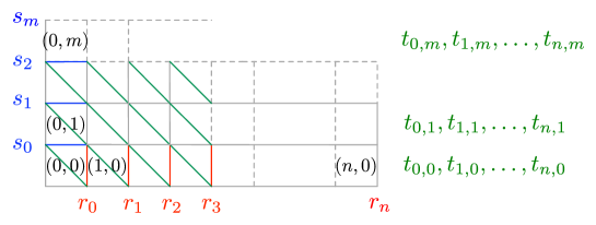
In [1], we derived a matrix model reproducing the topological string partition function on the toric Calabi-Yau geometry 𝔛0subscript𝔛0{\mathfrak{X}}_{0} whose toric fan is depicted in figure 1. We refer to 𝔛0subscript𝔛0{\mathfrak{X}}_{0} as our fiducial geometry; we will obtain the partition function on an arbitrary toric Calabi-Yau manifolds by considering flops and limits of 𝔛0subscript𝔛0{\mathfrak{X}}_{0}.

Refer to caption
Figure 1: Fiducial geometry 𝔛0subscript𝔛0{\mathfrak{X}}_{0} with boxes numbered and choice of basis of H2(𝔛0,)subscript𝐻2subscript𝔛0H_{2}({\mathfrak{X}}_{0},\mathbb{Z}).

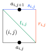
We have indicated a basis of H2(𝔛0,)subscript𝐻2subscript𝔛0H_{2}({\mathfrak{X}}_{0},\mathbb{Z}) in figure 1. Applying the labeling scheme introduced in figure 2, the curve classes of our geometry are expressed in this basis as follows,

ri,jsubscript𝑟𝑖𝑗\displaystyle r_{i,j} =\displaystyle= ri+k=1j(ti+1,k1ti,k)subscript𝑟𝑖superscriptsubscript𝑘1𝑗subscript𝑡𝑖1𝑘1subscript𝑡𝑖𝑘\displaystyle r_{i}+\sum_{k=1}^{j}(t_{i+1,k-1}-t_{i,k})
si,jsubscript𝑠𝑖𝑗\displaystyle s_{i,j} =\displaystyle= sj+k=1i(tk1,j+1tk,j).subscript𝑠𝑗superscriptsubscript𝑘1𝑖subscript𝑡𝑘1𝑗1subscript𝑡𝑘𝑗\displaystyle s_{j}+\sum_{k=1}^{i}(t_{k-1,j+1}-t_{k,j})\,.

It proves convenient to express these classes as differences of what we will refer to as a𝑎a-parameters [1], defined via

ti,j=ai,jai,j+1,ri,j=ai,j+1ai+1,j.t_{i,j}=a_{i,j}-a_{i,j+1}\quad\,,\quad\quad r_{i,j}=a_{i,j+1}-a_{i+1,j}\,.
Refer to caption
Figure 2: Labeling curve classes, and introducing a𝑎a-parameters.

2.2 The mirror of the fiducial geometry

The Hori-Vafa prescription [20] allows us to assign a mirror curve to a toric Calabi-Yau manifold. Each torically invariant divisor, corresponding to a 1-cone ρΣ(1)𝜌Σ1\rho\in\Sigma(1), is mapped to a superscript\mathbb{C}^{*} variable eYρsuperscript𝑒subscript𝑌𝜌e^{-Y_{\rho}}. These are constrained by the equation

ρΣ(1)eYρ=0.subscript𝜌Σ1superscript𝑒subscript𝑌𝜌0\sum_{\rho\in\Sigma(1)}e^{-Y_{\rho}}=0\,.

Relations between the 1-cones, as captured by the lattice ΛhsubscriptΛ\Lambda_{h} introduced in section (2.1) of [1], map to relations between these variables: for σΣ(2)𝜎Σ2\sigma\in\Sigma(2),

ρΣ(1)λρ(σ)Yρ=Wσ.subscript𝜌Σ1subscript𝜆𝜌𝜎subscript𝑌𝜌subscript𝑊𝜎\sum_{\rho\in\Sigma(1)}\lambda_{\rho}(\sigma)Y_{\rho}=W_{\sigma}\,. (2.1)

The Wσsubscript𝑊𝜎W_{\sigma} are complex structure parameters of the mirror geometry, related to the Kähler parameters wσ=ri,j,si,j,subscript𝑤𝜎subscript𝑟𝑖𝑗subscript𝑠𝑖𝑗w_{\sigma}=r_{i,j},s_{i,j},\ldots introduced in the previous subsection via the mirror map, as we will explain in the next subsection.

The Hori-Vafa prescription gives rise to the following mirror curve 𝒞𝔛0subscript𝒞subscript𝔛0{{\mathcal{C}}}_{{\mathfrak{X}}_{0}} of our fiducial geometry 𝔛0subscript𝔛0{\mathfrak{X}}_{0},

i=0n+1j=0m+1xi,j=0.superscriptsubscript𝑖0𝑛1superscriptsubscript𝑗0𝑚1subscript𝑥𝑖𝑗0\sum_{i=0}^{n+1}\sum_{j=0}^{m+1}x_{i,j}=0\,. (2.2)

We have here labeled the 1-cones by coordinates (i,j)𝑖𝑗(i,j), beginning with (0,0)00(0,0) for the cone (0,0,1)001(0,0,1) in the bottom left corner of box (0,0)00(0,0) as labeled in figure 1, and introduced the notation

xi,j=eYi,j.subscript𝑥𝑖𝑗superscript𝑒subscript𝑌𝑖𝑗x_{i,j}=e^{-Y_{i,j}}\,.

Eliminating dependent variables by invoking (2.1) yields an equation of the form

i=0n+1j=0m+1ci,jzi,j=0.superscriptsubscript𝑖0𝑛1superscriptsubscript𝑗0𝑚1subscript𝑐𝑖𝑗subscript𝑧𝑖𝑗0\sum_{i=0}^{n+1}\sum_{j=0}^{m+1}c_{i,j}z_{i,j}=0\,. (2.3)

Here,

zi,j=x01ijx1ix2j,subscript𝑧𝑖𝑗superscriptsubscript𝑥01𝑖𝑗superscriptsubscript𝑥1𝑖superscriptsubscript𝑥2𝑗z_{i,j}=x_{0}^{1-i-j}x_{1}^{i}x_{2}^{j}\,,

where we have defined

x0=x0,0,x1=x1,0,x2=x0,1.formulae-sequencesubscript𝑥0subscript𝑥00formulae-sequencesubscript𝑥1subscript𝑥10subscript𝑥2subscript𝑥01x_{0}=x_{0,0}\,,\,\,x_{1}=x_{1,0}\,,\,\,x_{2}=x_{0,1}\,.

(x0:x1:x2):subscript𝑥0subscript𝑥1:subscript𝑥2(x_{0}:x_{1}:x_{2}) define homogeneous coordinates on 2superscript2\mathbb{C}\mathbb{P}^{2}. The form of the equation is independent of the choice of triangulation of the toric diagram. What does depend on this choice are the coefficients ci,jsubscript𝑐𝑖𝑗c_{i,j}. It is not hard to write these down for the fiducial geometry 𝔛0subscript𝔛0{\mathfrak{X}}_{0} with the choice of basis for H2(𝔛0,)subscript𝐻2subscript𝔛0H_{2}({\mathfrak{X}}_{0},\mathbb{Z}) indicated in figure 1. Explicitly, the relations between the coordinates of the mirror curve (2.2) are

xi,0=xi1,0xi1,1xi2,1eRi2,x0,j=x0,j1x1,j1x1,j2eSj2,xi,j=xi1,jxi,j1xi1,j1eTi1,j1.formulae-sequencesubscript𝑥𝑖0subscript𝑥𝑖10subscript𝑥𝑖11subscript𝑥𝑖21superscript𝑒subscript𝑅𝑖2formulae-sequencesubscript𝑥0𝑗subscript𝑥0𝑗1subscript𝑥1𝑗1subscript𝑥1𝑗2superscript𝑒subscript𝑆𝑗2subscript𝑥𝑖𝑗subscript𝑥𝑖1𝑗subscript𝑥𝑖𝑗1subscript𝑥𝑖1𝑗1superscript𝑒subscript𝑇𝑖1𝑗1x_{i,0}=\frac{x_{i-1,0}x_{i-1,1}}{x_{i-2,1}}e^{R_{i-2}}\,,\quad x_{0,j}=\frac{x_{0,j-1}x_{1,j-1}}{x_{1,j-2}}e^{S_{j-2}}\,,\quad x_{i,j}=\frac{x_{i-1,j}x_{i,j-1}}{x_{i-1,j-1}}e^{T_{i-1,j-1}}\,. (2.4)

Solving in terms of x0,x1,x2subscript𝑥0subscript𝑥1subscript𝑥2x_{0},x_{1},x_{2} yields the coefficients c0,0=c0,1=c1,0=1subscript𝑐00subscript𝑐01subscript𝑐101c_{0,0}=c_{0,1}=c_{1,0}=1,

ci,0subscript𝑐𝑖0\displaystyle c_{i,0} =exp[k=1i1(ik)(Rk1+Tk1,0)],absentsuperscriptsubscript𝑘1𝑖1𝑖𝑘subscript𝑅𝑘1subscript𝑇𝑘10\displaystyle=\exp\left[\sum_{k=1}^{i-1}(i-k)(R_{k-1}+T_{k-1,0})\right]\,,
c0,jsubscript𝑐0𝑗\displaystyle c_{0,j} =exp[l=1j1(jl)(Sl1+T0,l1)],absentsuperscriptsubscript𝑙1𝑗1𝑗𝑙subscript𝑆𝑙1subscript𝑇0𝑙1\displaystyle=\exp\left[\sum_{l=1}^{j-1}(j-l)(S_{l-1}+T_{0,l-1})\right]\,,
and for i,j>0𝑖𝑗0i,j>0
ci,jsubscript𝑐𝑖𝑗\displaystyle c_{i,j} =exp[(i+j1)T0,0+k=1i1(ik)(Rk1+Tk,0)+l=1j1(jl)(Sl1+T0,l)+k=1i1l=1j1Tk,l].absent𝑖𝑗1subscript𝑇00superscriptsubscript𝑘1𝑖1𝑖𝑘subscript𝑅𝑘1subscript𝑇𝑘0superscriptsubscript𝑙1𝑗1𝑗𝑙subscript𝑆𝑙1subscript𝑇0𝑙superscriptsubscript𝑘1𝑖1superscriptsubscript𝑙1𝑗1subscript𝑇𝑘𝑙\displaystyle=\exp\left[(i+j-1)T_{0,0}+\sum_{k=1}^{i-1}(i-k)(R_{k-1}+T_{k,0})+\sum_{l=1}^{j-1}(j-l)(S_{l-1}+T_{0,l})+\sum_{k=1}^{i-1}\sum_{l=1}^{j-1}T_{k,l}\right]\,.

Note that the number of coefficients ci,jsubscript𝑐𝑖𝑗c_{i,j}, up to an overall rescaling, is equal to the number of independent curve classes risubscript𝑟𝑖r_{i}, sjsubscript𝑠𝑗s_{j}, ti,jsubscript𝑡𝑖𝑗t_{i,j}.

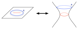
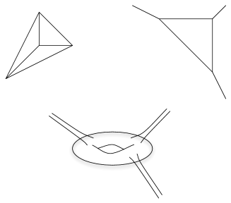
In [21], the thickening prescription was put forth for determining the genus and number of punctures of the mirror curve: one is to thicken the web diagram of the original geometry to obtain the Riemann surface of the mirror geometry. The procedure is illustrated in figure 3. We will now verify this procedure by studying the curve (2.3) explicitly.
Refer to caption
Figure 3: Example of the thickening prescription: depicted are the fan for 𝒪(3)2𝒪3superscript2{\cal O}(-3)\rightarrow\mathbb{P}^{2}, the corresponding web diagram, and the mirror curve obtained via the thickening prescription.

Let’s consider the curve (2.3) for a single strip (i.e. n=0𝑛0n=0) of length m+1𝑚1m+1,

x0m+2+x0m+1x1+x0m+1x2+c1,1x0mx1x2+c2,0x0mx12+c2,1x0m1x12x2+c3,0x0m1x13++cm+1,0x0x1m+1+cm+1,1x1m+1x2=0.superscriptsubscript𝑥0𝑚2superscriptsubscript𝑥0𝑚1subscript𝑥1superscriptsubscript𝑥0𝑚1subscript𝑥2subscript𝑐11superscriptsubscript𝑥0𝑚subscript𝑥1subscript𝑥2subscript𝑐20superscriptsubscript𝑥0𝑚superscriptsubscript𝑥12subscript𝑐21superscriptsubscript𝑥0𝑚1superscriptsubscript𝑥12subscript𝑥2subscript𝑐30superscriptsubscript𝑥0𝑚1superscriptsubscript𝑥13subscript𝑐𝑚10subscript𝑥0superscriptsubscript𝑥1𝑚1subscript𝑐𝑚11superscriptsubscript𝑥1𝑚1subscript𝑥20x_{0}^{m+2}+x_{0}^{m+1}x_{1}+x_{0}^{m+1}x_{2}+c_{1,1}\,x_{0}^{m}x_{1}x_{2}+c_{2,0}\,x_{0}^{m}x_{1}^{2}+c_{2,1}\,x_{0}^{m-1}x_{1}^{2}x_{2}+c_{3,0}\,x_{0}^{m-1}x_{1}^{3}+\ldots\\ +c_{m+1,0}\,x_{0}x_{1}^{m+1}+c_{m+1,1}\,x_{1}^{m+1}x_{2}=0\,. (2.5)

Note that the equation is of degree m+2𝑚2m+2, but the point (0:0:1):00:1(0:0:1) is an m+1𝑚1m+1-tuple point. By choosing the coefficients to be generic, we can arrange for this singular point to be ordinary. The genus formula then yields

𝔤=(d1)(d2)2m(m+1)2=0.𝔤𝑑1𝑑22𝑚𝑚120{\mathfrak{g}}=\frac{(d-1)(d-2)}{2}-\frac{m(m+1)}{2}=0\,.

In terms of the physical variables Yisubscript𝑌𝑖Y_{i}, any point on the curve with a vanishing homogeneous coordinate corresponds to a puncture. The punctures on the curve (2.5) thus lie at

(0:0:1):00:1\displaystyle(0:0:1)\quad :m+1:𝑚1\displaystyle:\quad m+1
(0:1:0):01:0\displaystyle(0:1:0)\quad :1:1\displaystyle:\quad 1
(1:x1i:0):1superscriptsubscript𝑥1𝑖:0\displaystyle(1:x_{1}^{i}:0)\quad :m+1:𝑚1\displaystyle:\quad m+1
(1:0:1):10:1\displaystyle(1:0:-1)\quad :1,:1\displaystyle:\quad 1\,,

where x1isuperscriptsubscript𝑥1𝑖x_{1}^{i}, i=1,,m+1𝑖1𝑚1i=1,\dots,m+1, are the solutions of the equation

1+x1+j=1mdix1i+11subscript𝑥1superscriptsubscript𝑗1𝑚subscript𝑑𝑖superscriptsubscript𝑥1𝑖1\displaystyle 1+x_{1}+\sum_{j=1}^{m}d_{i}x_{1}^{i+1} =\displaystyle= 0.0\displaystyle 0\,.

Note that we reproduce the 2m+42𝑚42m+4 punctures expected from the thickening prescription of the toric diagram.

For the general case parametrized by (m,n)𝑚𝑛(m,n), the degree of the curve is d=m+n+2𝑑𝑚𝑛2d=m+n+2, and we have an ordinary m+1𝑚1m+1-tuple point at (0:0:1):00:1(0:0:1) and an ordinary n+1𝑛1n+1-tuple point at (0:1:0):01:0(0:1:0). The genus formula now yields

g=(m+n)(m+n+1)2m(m+1)2n(n+1)2=mn.𝑔𝑚𝑛𝑚𝑛12𝑚𝑚12𝑛𝑛12𝑚𝑛g=\frac{(m+n)(m+n+1)}{2}-\frac{m(m+1)}{2}-\frac{n(n+1)}{2}=mn\,.

The punctures lie at

(0:0:1):00:1\displaystyle(0:0:1)\quad :m+1:𝑚1\displaystyle:\quad m+1
(0:1:0):01:0\displaystyle(0:1:0)\quad :n+1:𝑛1\displaystyle:\quad n+1
(1:x1i:0):1superscriptsubscript𝑥1𝑖:0\displaystyle(1:x_{1}^{i}:0)\quad :m+1:𝑚1\displaystyle:\quad m+1
(1:0:x2j):10:superscriptsubscript𝑥2𝑗\displaystyle(1:0:x_{2}^{j})\quad :n+1,:𝑛1\displaystyle:\quad n+1\,,

with x1isuperscriptsubscript𝑥1𝑖x_{1}^{i} the roots of i=0m+1ci,0x1i=0superscriptsubscript𝑖0𝑚1subscript𝑐𝑖0superscriptsubscript𝑥1𝑖0\sum_{i=0}^{m+1}c_{i,0}x_{1}^{i}=0 and x2jsuperscriptsubscript𝑥2𝑗x_{2}^{j} the roots of j=0n+1c0,jx2j=0superscriptsubscript𝑗0𝑛1subscript𝑐0𝑗superscriptsubscript𝑥2𝑗0\sum_{j=0}^{n+1}c_{0,j}x_{2}^{j}=0. Again, we see that we reproduce the thickening prescription.

2.3 The mirror map

Above, we have distinguished between Kähler (A𝐴A-model) parameters wσsubscript𝑤𝜎w_{\sigma} and complex structure (B𝐵B-model) parameters Wσsubscript𝑊𝜎W_{\sigma}. At large radius/complex structure, these are identified between mirror pairs, but this identification is corrected by the so-called mirror map,111One could take exception to this nomenclature, arguing that the parameters Wσsubscript𝑊𝜎W_{\sigma} are the geometric parameters on both sides of the mirror, and refer to the wσsubscript𝑤𝜎w_{\sigma} as the instanton or quantum corrected parameters. In such conventions, the curve classes in the various toric diagrams should be labeled by upper case letters.

Wσ=wσ+𝒪(ewσ).subscript𝑊𝜎subscript𝑤𝜎𝒪superscript𝑒subscript𝑤𝜎W_{\sigma}=w_{\sigma}+{\cal O}(e^{-w_{\sigma}})\,. (2.6)

The exponentials of the parameters Wσsubscript𝑊𝜎W_{\sigma} appear as coefficients in the equation defining the mirror curve. They are global coordinates on the complex structure moduli space of the mirror curve. To compare expressions obtained in the A-model to those obtained in the B-model, all expressions are conventionally expressed in terms of flat coordinates wσsubscript𝑤𝜎w_{\sigma}. On the A-model side, these coordinates enter (in exponentiated form denoted generically as Qα,βsubscript𝑄𝛼𝛽Q_{\alpha,\beta} below) in the definition of the topological vertex. On the B-model side, they arise as the appropriate periods of a meromorphic one-form λ𝜆\lambda, defined in terms of the affine variables x=x1x0𝑥subscript𝑥1subscript𝑥0x=\frac{x_{1}}{x_{0}}, y=x2x0𝑦subscript𝑥2subscript𝑥0y=\frac{x_{2}}{x_{0}} in the patch x00subscript𝑥00x_{0}\neq 0 of the curve (2.3) as

λ=logydxx.𝜆𝑦𝑑𝑥𝑥\lambda=\log y\frac{dx}{x}\,.

By calculating these periods as a function of the coefficients defining the mirror curve, we obtain the mirror map (2.6).

The coordinates wσsubscript𝑤𝜎w_{\sigma} are not globally defined functions on the complex structure moduli space. In the slightly clearer compact setting, this is due to the fact that the symplectic basis {αA,βA}subscript𝛼𝐴superscript𝛽𝐴\{\alpha_{A},\beta^{A}\} of H3(𝔛,)superscript𝐻3𝔛H^{3}({\mathfrak{X}},\mathbb{Z}) in which we expand ΩΩ\Omega (the compact analogue of the meromorphic 1-form λ𝜆\lambda introduced above) such that the coefficients of αAsubscript𝛼𝐴\alpha_{A} furnish our (local) coordinate system of the complex structure moduli space, undergo monodromy when transported around a singularity in moduli space.222Note that the symplectic basis makes no reference to complex structure, one might hence be led to believe that a global choice (i.e. one valid for any choice of complex structure) should be possible. This is not so. We consider the family π:𝒳𝒮:𝜋𝒳𝒮\pi:{\cal X}\rightarrow{\cal S}, with 𝒮𝒮{\cal S} the complex structure moduli space. The fiber over each point w𝒮𝑤𝒮w\in{\cal S}, π1w=Xwsuperscript𝜋1𝑤subscript𝑋𝑤\pi^{-1}w=X_{w}, is the Calabi-Yau manifold with the respective complex structure. Hn(Xw,)superscript𝐻𝑛subscript𝑋𝑤H^{n}(X_{w},\mathbb{C}) fit together to form a vector bundle 0subscript0{\cal F}_{0} over 𝒮𝒮{\cal S}, with a canonical flat connection, the Gauss-Manin connection. Using this connection, we can parallel transport a symplectic basis of H3(Xw,)superscript𝐻3subscript𝑋𝑤H^{3}(X_{w},\mathbb{C}) along a curve in 𝒮𝒮{\cal S}. As 𝒮𝒮{\cal S} is not generically simply connected (due to the existence of degeneration points of the geometry), this transport may exhibit monodromy. Note that ΩΩ\Omega can be defined as the section of a sheaf in the Hodge filtration of H3superscript𝐻3H^{3} which extends to the singular divisor, hence is single valued. The monodromy in our choice of flat coordinates is therefore entirely due to the choice of symplectic basis. A good choice of coordinates in the vicinity of a singular divisor D𝐷D hence involves a choice of basis forms that are invariant under monodromy around that divisor.

3 Our matrix model

We derived a chain of matrices matrix model that reproduces the topological string partition function on 𝔛0subscript𝔛0{\mathfrak{X}}_{0} in [1]. For 𝔛0subscript𝔛0{\mathfrak{X}}_{0} of size (n+1)×(m+1)𝑛1𝑚1(n+1)\times(m+1), as depicted in figure 1, it is given by

ZMM(Q,gs,αm+1,α0T)subscript𝑍MM𝑄subscript𝑔𝑠subscript𝛼𝑚1superscriptsubscript𝛼0𝑇\displaystyle{Z}_{\rm MM}(\vec{Q},g_{s},\vec{\alpha}_{m+1},\vec{\alpha}_{0}^{T}) =\displaystyle= Δ(X(αm+1))Δ(X(α0))i=0m+1HN(Γi)𝑑Mii=1m+1HN(+)𝑑RiΔ𝑋subscript𝛼𝑚1Δ𝑋subscript𝛼0superscriptsubscriptproduct𝑖0𝑚1subscriptsubscript𝐻𝑁subscriptΓ𝑖differential-dsubscript𝑀𝑖superscriptsubscriptproduct𝑖1𝑚1subscriptsubscript𝐻𝑁subscriptdifferential-dsubscript𝑅𝑖\displaystyle\Delta(X(\vec{\alpha}_{m+1}))\,\,\Delta(X(\vec{\alpha}_{0}))\,\,\prod_{i=0}^{m+1}\int_{H_{N}(\Gamma_{i})}dM_{i}\,\prod_{i=1}^{m+1}\int_{H_{N}({\mathbb{R}}_{+})}\,dR_{i} (3.1)
i=1me1gstr[Vai(Mi)Vai1(Mi)]i=1me1gstr[Vai1(Mi1)Vai(Mi1)]superscriptsubscriptproduct𝑖1𝑚superscript𝑒1subscript𝑔𝑠trdelimited-[]subscript𝑉subscript𝑎𝑖subscript𝑀𝑖subscript𝑉subscript𝑎𝑖1subscript𝑀𝑖superscriptsubscriptproduct𝑖1𝑚superscript𝑒1subscript𝑔𝑠trdelimited-[]subscript𝑉subscript𝑎𝑖1subscript𝑀𝑖1subscript𝑉subscript𝑎𝑖subscript𝑀𝑖1\displaystyle\prod_{i=1}^{m}e^{{-1\over g_{s}}\,{\rm tr\,}\left[V_{\vec{a}_{i}}(M_{i})-V_{\vec{a}_{i-1}}(M_{i})\right]}\,\,\,\prod_{i=1}^{m}e^{{-1\over g_{s}}\,{\rm tr\,}\left[V_{\vec{a}_{i-1}}(M_{i-1})-V_{\vec{a}_{i}}(M_{i-1})\right]}
i=1m+1e1gstr(MiMi1)Rii=1me(Si+iπgs)trlnMisuperscriptsubscriptproduct𝑖1𝑚1superscript𝑒1subscript𝑔𝑠trsubscript𝑀𝑖subscript𝑀𝑖1subscript𝑅𝑖superscriptsubscriptproduct𝑖1𝑚superscript𝑒subscript𝑆𝑖𝑖𝜋subscript𝑔𝑠trsubscript𝑀𝑖\displaystyle\prod_{i=1}^{m+1}e^{{1\over g_{s}}{\rm tr\,}(M_{i}-M_{i-1})R_{i}}\,\,\,\prod_{i=1}^{m}e^{(S_{i}+{i\pi\over g_{s}})\,{\rm tr\,}\,\ln M_{i}}\,
etrlnf0(M0)etrlnfm+1(Mm+1)i=1metrlnfi(Mi).superscript𝑒trsubscript𝑓0subscript𝑀0superscript𝑒trsubscript𝑓𝑚1subscript𝑀𝑚1superscriptsubscriptproduct𝑖1𝑚superscript𝑒trsubscript𝑓𝑖subscript𝑀𝑖\displaystyle e^{{\rm tr\,}\ln f_{0}(M_{0})}\,\,e^{{\rm tr\,}\ln f_{m+1}(M_{m+1})}\,\,\prod_{i=1}^{m}e^{{\rm tr\,}\ln f_{i}(M_{i})}\,.

We give the explicit expressions for the various functions entering in this definition in appendix A. Here, we briefly explain some of its general features.

The matrix model (3.1) is designed to reproduce the topological string partition function on the toric Calabi-Yau manifold 𝔛0subscript𝔛0{\mathfrak{X}}_{0} as computed using the topological vertex [22]. Recall that in this formalism, the dual web diagram to the toric diagram underlying the geometry is decomposed into trivalent vertices. Each such vertex contributes a factor C(αi,αj,αkC(\alpha_{i},\alpha_{j},\alpha_{k}) [22], where αisubscript𝛼𝑖\alpha_{i} denote Young tableaux (partitions) of arbitrary size, one associated to each leg of the vertex. Legs of different vertices are glued by matching these Young tableaux and summing over them with appropriate weight.

Aside from the coupling constant gssubscript𝑔𝑠g_{s} and Kähler parameters of the geometry, denoted collectively as Q𝑄\vec{Q}, the matrix model (3.1) depends on partitions α0subscript𝛼0\vec{\alpha}_{0}, αm+1subscript𝛼𝑚1\vec{\alpha}_{m+1} associated to the outer legs of the web diagram, which we choose to be trivial in this paper. The two classes of integrals dRi𝑑subscript𝑅𝑖dR_{i} and dMi𝑑subscript𝑀𝑖dM_{i} correspond to the two steps in which the topological string partition function on the fiducial geometry 𝔛0subscript𝔛0{\mathfrak{X}}_{0} can be evaluated: First, the geometry can be decomposed into m+1𝑚1m+1 horizontal strips, with partitions αj,i+1subscript𝛼𝑗𝑖1\alpha_{j,i+1} and αj,isubscript𝛼𝑗𝑖\alpha_{j,i} associated to the upper and lower outer legs of the associated strip web diagram. j=0,,n𝑗0𝑛j=0,\ldots,n counts the boxes in figure 1 in the horizontal direction, i=0,,m+1𝑖0𝑚1i=0,\ldots,m+1 is essentially the strip index. Each such strip has a dRi𝑑subscript𝑅𝑖dR_{i} integration associated to it. The partition function on such strips was calculated in [23]. Following [12], we introduce two matrices Misubscript𝑀𝑖M_{i}, Mi+1subscript𝑀𝑖1M_{i+1} per strip. Their eigenvalues encode the partitions αj,isubscript𝛼𝑗𝑖\alpha_{j,i} and αj,i+1subscript𝛼𝑗𝑖1\alpha_{j,i+1} for all j𝑗j. To work with finite size matrices, we introduce a cut-off d𝑑d on the number of rows of the Young tableaux we sum over. As we argue in section 5.2.1, our matrix model depends on d𝑑d only non-perturbatively. The strip partition function is essentially given by the Cauchy determinant of the two matrices Misubscript𝑀𝑖M_{i}, Mi+1subscript𝑀𝑖1M_{i+1} [1], and the dRi𝑑subscript𝑅𝑖dR_{i} integrals are the associated Laplace transforms. Gluing the strips together involves summing over the partitions αj,isubscript𝛼𝑗𝑖\alpha_{j,i}. This step is implemented by the dMi𝑑subscript𝑀𝑖dM_{i} integrations. To obtain a discrete sum over partitions from integration, we introduce functions fi(Mi)subscript𝑓𝑖subscript𝑀𝑖f_{i}(M_{i}) with integrally spaced poles. Integrating Misubscript𝑀𝑖M_{i} along appropriate contours then yields the sum over partitions as a sum over residues, the potentials Vaisubscript𝑉subscript𝑎𝑖V_{\vec{a}_{i}} chosen to provide the proper weight per partition.

4 Generalities on solving matrix models

4.1 Introduction to the topological expansion of chain of matrices

Chain of matrices matrix models have been extensively studied (see Mehta’s book [24] and the review article [25]), and the computation of their topological expansion was performed recently in [26, 27].

The solution provided in [27] is based on the computation of the spectral curve 𝒮MMsubscript𝒮MM{{\mathcal{S}}_{\rm MM}} of the matrix model. In [27, 26], only the case of potentials whose derivatives are rational functions is considered, and similarly to the one matrix model, the planar333For matrix models with N𝑁N-independent polynomial potentials whose gssubscript𝑔𝑠g_{s} dependence is given by an overall prefactor, the planar limit coincides with the large N𝑁N limit, but this correspondence can fail if the potential or the integration contours have a non-trivial N𝑁N or gssubscript𝑔𝑠g_{s} dependence. The planar limit is defined by keeping only planar graphs in the Feynman graph perturbative expansion around an extremum of the potential. However, it is helpful to have in mind the intuitive picture that the planar limit is similar to a large N𝑁N limit. expectation value of the resolvent of the first matrix of the chain is shown to satisfy an algebraic equation. The spectral curve is defined to be the solution locus of this equation. A general recipe is provided in [26, 27] to obtain the spectral curve from algebraic equations and analyticity properties related to rational potentials and integration contours. Here, our potentials contain logs of g𝑔g-functions. As they are not rational, we will have to present a slight extension of the recipe of [27] in section 4.2.2. This extension from rational potentials to analytical potentials, although not published, is straightforward, and the derivation of these results will appear in [28]. In some sense, the derivative of lng(x)𝑔𝑥\ln g(x) can be viewed as a rational function with an infinite number of simple poles, i.e. as a limit of a rational function. More precisely, as an expansion in powers of q𝑞q, to each order, it is a rational function. Since the spectral curve can be described by local properties, independent of the number of poles, one can take the limit of the recipe of [26, 27]. This is what we shall do in section 4.2.2 below.

Having found the spectral curve 𝒮MMsubscript𝒮MM{{\mathcal{S}}_{\rm MM}} of the matrix model, we will compute its symplectic invariants

Fg(𝒮MM),g=0,1,2,3,formulae-sequencesubscript𝐹𝑔subscript𝒮MM𝑔0123F_{g}({{\mathcal{S}}_{\rm MM}})\,,\quad g=0,1,2,3,\dots

Symplectic invariants Fg(𝒮)subscript𝐹𝑔𝒮F_{g}({{\mathcal{S}}}) can be computed for any analytical plane curve 𝒮𝒮{{\mathcal{S}}}, and thus in particular for 𝒮=𝒮MM𝒮subscript𝒮MM{{\mathcal{S}}}={{\mathcal{S}}_{\rm MM}}. For a general 𝒮𝒮{{\mathcal{S}}} they were first introduced in [3], as a generalization of the solution of matrix models loop equations of [2]. Their definition is algebraic and involves computation of residues at branch points of 𝒮𝒮{{\mathcal{S}}}. We recall the definition below in section 4.3.

4.2 Definition of the general chain of matrices

We consider chain of matrices matrix models of the form

Z=𝑑M1𝑑MLe1gsTri=1LVi(Mi)e1gsTri=1L1ciMiMi+1.𝑍subscriptdifferential-dsubscript𝑀1differential-dsubscript𝑀𝐿superscript𝑒1subscript𝑔𝑠Trsuperscriptsubscript𝑖1𝐿subscript𝑉𝑖subscript𝑀𝑖superscript𝑒1subscript𝑔𝑠Trsuperscriptsubscript𝑖1𝐿1subscript𝑐𝑖subscript𝑀𝑖subscript𝑀𝑖1Z=\int_{{\cal E}}dM_{1}\dots dM_{L}\,\,e^{-{1\over g_{s}}{\rm Tr\,}\sum_{i=1}^{L}V_{i}(M_{i})}\,\,e^{{1\over g_{s}}{\rm Tr\,}\sum_{i=1}^{L-1}c_{i}M_{i}M_{i+1}}\,. (4.1)

Note that aside from the potentials Vi(Mi)subscript𝑉𝑖subscript𝑀𝑖V_{i}(M_{i}), the only interactions are between nearest neighbors, whence the name “chain of matrices.” Chain of matrices matrix models can be solved when the interaction terms between different matrices are of the form TrMiMi+1Trsubscript𝑀𝑖subscript𝑀𝑖1{\rm Tr\,}M_{i}M_{i+1}, as is the case here.

{\cal E} can be any ensemble of L𝐿L normal matrices of size N×N𝑁𝑁N\times N, i.e. a submanifold of LN2superscript𝐿superscript𝑁2\mathbb{C}^{LN^{2}} of real dimension LN2𝐿superscript𝑁2LN^{2}, such that the integral is convergent. {\cal E} can be many things; for a chain of matrices model, it is characterized by the contours on which eigenvalues of the various normal matrices are integrated (see [29] for the 2-matrix model case). For (4.1) to have a topological expansion, {\cal E} must be a so-called steepest descent ensemble (see [30], section 5.5). For a generic ensemble {\cal E} which would not be steepest descent, lnZ𝑍\ln Z would be an oscillating function of 1/gs1subscript𝑔𝑠1/g_{s}, and no small gssubscript𝑔𝑠g_{s} expansion would exist, see [31].

The matrix model introduced in [1] and reproduced in section 3 was defined to reproduce the topological string partition function, which is defined as a formal series in gssubscript𝑔𝑠g_{s}, and therefore has a topological expansion by construction.

An ensemble {\cal E} is characterized by filling fractions nj,isubscript𝑛𝑗𝑖n_{j,i},

=i=1Li,i=HN(γ1,in1,i×γ2,in2,i××γki,inki,i),{\cal E}=\prod_{i=1}^{L}{\cal E}_{i}\quad,\quad{\cal E}_{i}=H_{N}(\gamma_{1,i}^{n_{1,i}}\times\gamma_{2,i}^{n_{2,i}}\times\dots\times\gamma_{k_{i},i}^{n_{k_{i},i}})\,, (4.2)

where HN(γ1n1××γknk)subscript𝐻𝑁superscriptsubscript𝛾1subscript𝑛1superscriptsubscript𝛾𝑘subscript𝑛𝑘H_{N}(\gamma_{1}^{n_{1}}\times\dots\times\gamma_{k}^{n_{k}}) is the set of normal matrices with n1subscript𝑛1n_{1} eigenvalues on path γ1subscript𝛾1\gamma_{1}, n2subscript𝑛2n_{2} eigenvalues on path γ2subscript𝛾2\gamma_{2}, \dots, nksubscript𝑛𝑘n_{k} eigenvalues on path γksubscript𝛾𝑘\gamma_{k}.

As the filling fractions nj,isubscript𝑛𝑗𝑖n_{j,i} must satisfy the relation

j=1kinj,i=Nsuperscriptsubscript𝑗1subscript𝑘𝑖subscript𝑛𝑗𝑖𝑁\sum_{j=1}^{k_{i}}n_{j,i}=N

for all i𝑖i, only i(ki1)subscript𝑖subscript𝑘𝑖1\sum_{i}(k_{i}-1) of them are independent.

We also allow some paths γj,isubscript𝛾𝑗𝑖\gamma_{j,i} to have endpoints where eTri=1L(Vi(Mi)MiMi+1)0superscript𝑒Trsuperscriptsubscript𝑖1𝐿subscript𝑉𝑖subscript𝑀𝑖subscript𝑀𝑖subscript𝑀𝑖10e^{-{\rm Tr\,}\sum_{i=1}^{L}(V_{i}(M_{i})-M_{i}M_{i+1})}\neq 0 – indeed, in our matrix model, the matrices Risubscript𝑅𝑖R_{i} are integrated on H(+N)𝐻superscriptsubscript𝑁H(\mathbb{R}_{+}^{N}).

4.2.1 The resolvent

The spectral curve encodes all Wi(x)subscript𝑊𝑖𝑥W_{i}(x), the planar limits (see footnote 3) of the resolvents of the matrices Misubscript𝑀𝑖M_{i},

Wi(x)=gstr1xMiplanar,subscript𝑊𝑖𝑥subscript𝑔𝑠subscriptdelimited-⟨⟩tr1𝑥subscript𝑀𝑖𝑝𝑙𝑎𝑛𝑎𝑟W_{i}(x)=g_{s}\,\left<{\rm tr\,}{1\over x-M_{i}}\right>_{planar}\,,

see equation (4.5) below. The respective Wisubscript𝑊𝑖W_{i} can be expressed as the Stieljes transform

Wi(x)=ρi(x)dxxxsubscript𝑊𝑖𝑥subscript𝜌𝑖superscript𝑥𝑑superscript𝑥𝑥superscript𝑥W_{i}(x)=\int{\rho_{i}(x^{\prime})dx^{\prime}\over x-x^{\prime}}

of the planar expectation value of the eigenvalue density ρi(x)subscript𝜌𝑖𝑥\rho_{i}(x) of the matrix Misubscript𝑀𝑖M_{i},

ρi(x)=gstrδ(xMi)planar.subscript𝜌𝑖𝑥subscript𝑔𝑠subscriptdelimited-⟨⟩tr𝛿𝑥subscript𝑀𝑖𝑝𝑙𝑎𝑛𝑎𝑟\rho_{i}(x)=g_{s}\,\left<{\rm tr\,}\delta(x-M_{i})\right>_{planar}\,.

By general properties of Stieljes transforms, singularities of Wi(x)subscript𝑊𝑖𝑥W_{i}(x) coincide with the support of the distribution ρi(x)dxsubscript𝜌𝑖𝑥𝑑𝑥\rho_{i}(x)dx:

  • Simple poles of Wi(x)subscript𝑊𝑖𝑥W_{i}(x) correspond to delta distributions i.e. isolated eigenvalues.

  • Multiple poles correspond to higher derivatives of delta distributions.

  • Cuts correspond to finite densities, the density being the discontinuity of Wi(x)subscript𝑊𝑖𝑥W_{i}(x) along the cut,

    ρi(x)=12iπ(Wi(xi0)Wi(x+i0)).subscript𝜌𝑖𝑥12𝑖𝜋subscript𝑊𝑖𝑥𝑖0subscript𝑊𝑖𝑥𝑖0\rho_{i}(x)={1\over 2i\pi}\,(W_{i}(x-i0)-W_{i}(x+i0))\,. (4.3)

In particular, cuts emerging from algebraic singularities (generically square root singularities) correspond to densities vanishing algebraically (generically as square roots) at the endpoints of the cut. Cuts emerging from logarithmic singularities correspond to constant densities.

4.2.2 The spectral curve of the general chain of matrices

When all Visubscriptsuperscript𝑉𝑖V^{\prime}_{i} are rational, the spectral curve was found in [26, 27], and it is algebraic. We present here a generalization of this result to more general potentials. The derivations of these results will appear in [28].

The spectral curve can be obtained by the following procedure:

  1. 1.

    Consider a compact Riemann surface 𝒞𝒞{{\mathcal{C}}} of genus

    𝔤=i=1L(ki1),𝔤superscriptsubscript𝑖1𝐿subscript𝑘𝑖1{\mathfrak{g}}=\sum_{i=1}^{L}(k_{i}-1)\,,

    where kisubscript𝑘𝑖k_{i} denotes the number of cuts of the i𝑖i-th matrix, as implicitly defined in (4.2).

  2. 2.

    Look for L+2𝐿2L+2 functions on 𝒞𝒞{{\mathcal{C}}},

    x0(z),x1(z),x2(z),,xL(z),xL+1(z):𝒞1.:subscript𝑥0𝑧subscript𝑥1𝑧subscript𝑥2𝑧subscript𝑥𝐿𝑧subscript𝑥𝐿1𝑧𝒞superscript1x_{0}(z),\,x_{1}(z),\,x_{2}(z),\,\dots,\,x_{L}(z),\,x_{L+1}(z):{{\mathcal{C}}}\rightarrow\mathbb{C}\mathbb{P}^{1}\,.

    The xisubscript𝑥𝑖x_{i} are to be holomorphic away from points z𝒞𝑧𝒞z\in{{\mathcal{C}}} at which Vi1(xi1)subscriptsuperscript𝑉𝑖1subscript𝑥𝑖1V^{\prime}_{i-1}(x_{i-1}) or Vi+1(xi+1)subscriptsuperscript𝑉𝑖1subscript𝑥𝑖1V^{\prime}_{i+1}(x_{i+1}) become singular, and satisfy the functional relations

    ci1xi1(z)+cixi+1(z)=Vi(xi(z)).subscript𝑐𝑖1subscript𝑥𝑖1𝑧subscript𝑐𝑖subscript𝑥𝑖1𝑧subscriptsuperscript𝑉𝑖subscript𝑥𝑖𝑧c_{i-1}x_{i-1}(z)+c_{i}x_{i+1}(z)=V^{\prime}_{i}(x_{i}(z))\,. (4.4)

    Recall that the cisubscript𝑐𝑖c_{i} are the coefficients of the interaction potentials in (4.1). We have set c0=cL=1subscript𝑐0subscript𝑐𝐿1c_{0}=c_{L}=1.

    For each i=1,,L𝑖1𝐿i=1,\dots,L, the Riemann surface 𝒞𝒞{{\mathcal{C}}} can be realized as a branched covering of 1superscript1\mathbb{C}\mathbb{P}^{1} by the projection xi:𝒞1:subscript𝑥𝑖𝒞superscript1x_{i}:{{\mathcal{C}}}\to\mathbb{C}\mathbb{P}^{1}. A choice of branched covering is not unique: the choice consists in the set of cuts connecting branch points (recall that these are points at which dxi(z)=0𝑑subscript𝑥𝑖𝑧0dx_{i}(z)=0). We will determine an appropriate covering below in step 4.

  3. 3.

    If some path γj,isubscript𝛾𝑗𝑖\gamma_{j,i} has an endpoint a𝑎a (called “hard edge” in the matrix model literature, see [32]), then choose a pre-image aixi1(a)subscript𝑎𝑖superscriptsubscript𝑥𝑖1𝑎a_{i}\in x_{i}^{-1}(a) and require

    dxi(ai)=0andxi1(z)hasasimplepoleatz=ai.formulae-sequence𝑑subscript𝑥𝑖subscript𝑎𝑖0andsubscript𝑥𝑖1𝑧hasasimplepoleat𝑧subscript𝑎𝑖dx_{i}(a_{i})=0\quad{\rm and}\quad x_{i-1}(z)\,\,{\rm has\,a\,simple\,pole\,at\,}z=a_{i}.

    The topological recursion is proved in [27] without hard edges, but it is not difficult to see, by mixing the results of [32], [33] and [27], that the topological recursion continues to hold in the presence of hard edges. The proof will appear in a forthcoming publication [28]. Here, we shall assume that it holds.

  4. 4.

    Choose some contours 𝒜^j,isubscript^𝒜𝑗𝑖\widehat{\cal A}_{j,i}, j=1,,ki𝑗1subscript𝑘𝑖j=1,\dots,k_{i} in 1superscript1\mathbb{C}\mathbb{P}^{1}, such that each 𝒜^j,isubscript^𝒜𝑗𝑖\widehat{\cal A}_{j,i} surrounds all points of the contour γj,isubscript𝛾𝑗𝑖\gamma_{j,i} (related to the matrix ensemble isubscript𝑖{\cal E}_{i} defined in (4.2)) in the clockwise direction and no other contour γj,isubscript𝛾superscript𝑗𝑖\gamma_{j^{\prime},i}. For x1𝑥superscript1x\in\mathbb{C}\mathbb{P}^{1} not enclosed in the contours 𝒜^j,isubscript^𝒜𝑗𝑖\widehat{{\cal A}}_{j,i}, j=1,,ki,𝑗1subscript𝑘𝑖j=1,\dots,k_{i}, and given a connected component 𝒜j,isubscript𝒜𝑗𝑖{{\cal A}_{j,i}} of the pre-image of the contour 𝒜^j,isubscript^𝒜𝑗𝑖\widehat{{\cal A}}_{j,i} under xisubscript𝑥𝑖x_{i},

    𝒜j,ixi1(𝒜^j,i),subscript𝒜𝑗𝑖superscriptsubscript𝑥𝑖1subscript^𝒜𝑗𝑖{\cal A}_{j,i}\subset x_{i}^{-1}(\widehat{{\cal A}}_{j,i})\,,

    define the function

    Wi(x)=ci12iπj=1ki𝒜j,ixi1(z)dxi(z)xxi(z).subscript𝑊𝑖𝑥subscript𝑐𝑖12𝑖𝜋superscriptsubscript𝑗1subscript𝑘𝑖subscriptcontour-integralsubscript𝒜𝑗𝑖subscript𝑥𝑖1𝑧𝑑subscript𝑥𝑖𝑧𝑥subscript𝑥𝑖𝑧W_{i}(x)={c_{i-1}\over 2i\pi}\sum_{j=1}^{k_{i}}\,\oint_{{\cal A}_{j,i}}\,\,{x_{i-1}(z)\,dx_{i}(z)\over x-x_{i}(z)}. (4.5)

    Generalizing [26] to non-polynomial potentials, we claim that a choice of 𝒜j,isubscript𝒜𝑗𝑖{\cal A}_{j,i} exists such that Wi(x)subscript𝑊𝑖𝑥W_{i}(x) is the planar limit of the resolvent of the matrix Misubscript𝑀𝑖M_{i}. In the following, it is this choice that will be referred to as 𝒜j,isubscript𝒜𝑗𝑖{\cal A}_{j,i}.

    Notice that not all 𝒜j,isubscript𝒜𝑗𝑖{\cal A}_{j,i} will be homologically independent on 𝒞𝒞{{\mathcal{C}}}. We require that we have 𝔤=i=1L(ki1)𝔤superscriptsubscript𝑖1𝐿subscript𝑘𝑖1\mathfrak{g}=\sum_{i=1}^{L}(k_{i}-1) homologically independent 𝒜j,isubscript𝒜𝑗𝑖{\cal A}_{j,i}’s, which coincides with the genus of 𝒞𝒞{{\mathcal{C}}}. As a condition on the choice of branched covering, we impose that 𝒜j,isubscript𝒜𝑗𝑖{\cal A}_{j,i} and aisubscript𝑎𝑖a_{i} lie on the same sheet of xisubscript𝑥𝑖x_{i}. This condition, in our experience, uniquely fixes this choice. We will assume that this is the case. We refer to the sheet of xisubscript𝑥𝑖x_{i} containing 𝒜j,isubscript𝒜𝑗𝑖{\cal A}_{j,i} and aisubscript𝑎𝑖a_{i} as the physical sheet for xisubscript𝑥𝑖x_{i}.

  5. 5.

    In accord with (4.3), we consider the discontinuity of Wi(x)subscript𝑊𝑖𝑥W_{i}(x) along the j𝑗j-th cut. It is given by

    DiscjWi(x)subscriptDisc𝑗subscript𝑊𝑖𝑥\displaystyle\mathop{{\rm Disc}\,}_{j}\,W_{i}(x) =\displaystyle= 12πi(Wi(x+)Wi(x))12𝜋𝑖subscript𝑊𝑖subscript𝑥subscript𝑊𝑖subscript𝑥\displaystyle\frac{1}{2\pi i}\left(W_{i}(x_{+})-W_{i}(x_{-})\right) (4.6)
    =\displaystyle= 12πici1Discjxi1,12𝜋𝑖subscript𝑐𝑖1subscriptDisc𝑗subscript𝑥𝑖1\displaystyle\frac{1}{2\pi i}c_{i-1}\,\mathop{{\rm Disc}\,}_{j}\,x_{i-1}\,,

    as we explain in figure 5.

    Refer to caption
    Figure 4: The integration contour 𝒜^j,isubscript^𝒜𝑗𝑖\widehat{\cal A}_{j,i} on the x𝑥x-plane, and its image 𝒜j,isubscript𝒜𝑗𝑖{\cal A}_{j,i} on 𝒞𝒞{{\mathcal{C}}}.
    Refer to caption
    Figure 5: The preimage of the points x+subscript𝑥x_{+} and xsubscript𝑥x_{-} of (4.6) are depicted as dots in the above diagram, 𝒜^j,isubscript^𝒜𝑗𝑖\widehat{{\cal A}}_{j,i} is given by the blue contour, and the preimage of the cut is drawn in red. To take the limit x+xsubscript𝑥subscript𝑥x_{+}\rightarrow x_{-}, one must first shift the contours. The second and fourth term on the RHS of the above diagrammatic equation then cancel, yielding the RHS of (4.6).

    The definition (4.2) of the matrix ensemble isubscript𝑖{\cal E}_{i} is the condition that there are nj,isubscript𝑛𝑗𝑖n_{j,i} eigenvalues of Misubscript𝑀𝑖M_{i} on the contour γj,isubscript𝛾𝑗𝑖\gamma_{j,i}, hence corresponds to imposing the filling fraction conditions

    12πi𝒜j,ici1xi1𝑑xi=gsnj,i12𝜋𝑖subscriptcontour-integralsubscript𝒜𝑗𝑖subscript𝑐𝑖1subscript𝑥𝑖1differential-dsubscript𝑥𝑖subscript𝑔𝑠subscript𝑛𝑗𝑖\frac{1}{2\pi i}\oint_{{\cal A}_{j,i}}c_{i-1}x_{i-1}dx_{i}=g_{s}\,\,n_{j,i}

    for i=1,,L𝑖1𝐿i=1,\dots,L, j=1,,ki𝑗1subscript𝑘𝑖j=1,\dots,k_{i}.


In our experience, the conditions enumerated above have a unique solution and define a unique spectral curve. As emphasized in the introduction, a formal uniqueness proof is however still lacking.

The spectral curve is defined as the data of the Riemann surface 𝒞𝒞{{\mathcal{C}}}, and the two functions x1(z)subscript𝑥1𝑧x_{1}(z) and x2(z)subscript𝑥2𝑧x_{2}(z),

   𝒮MM=(𝒞,x1,x2).subscript𝒮𝑀𝑀𝒞subscript𝑥1subscript𝑥2\displaystyle{{\mathcal{S}}}_{MM}=({{\mathcal{C}}},x_{1},x_{2}).    (4.7)

4.3 Symplectic invariants of a spectral curve

Once we have found the spectral curve 𝒮MMsubscript𝒮𝑀𝑀{{\mathcal{S}}}_{MM} of our matrix model, we can compute the coefficients Fgsubscript𝐹𝑔F_{g} in the topological expansion of its partition function,

lnZ=g=0gs2g2Fg,𝑍superscriptsubscript𝑔0superscriptsubscript𝑔𝑠2𝑔2subscript𝐹𝑔\ln Z=\sum_{g=0}^{\infty}g_{s}^{2g-2}F_{g}\,,

by computing the symplectic invariants of this curve,

Fg=Fg(𝒮MM),subscript𝐹𝑔subscript𝐹𝑔subscript𝒮𝑀𝑀F_{g}=F_{g}({{\mathcal{S}}}_{MM})\,,

following [27].

Let us recall the definition of these invariants for an arbitrary spectral curve 𝒮𝒮{{\mathcal{S}}}.

Let 𝒮=(𝒞,x,y)𝒮𝒞𝑥𝑦{{\mathcal{S}}}=({{\mathcal{C}}},x,y) be a spectral curve, comprised of the data of a Riemann surface 𝒞𝒞{{\mathcal{C}}} and two functions x(z),y(z):𝒞:𝑥𝑧𝑦𝑧𝒞x(z),\,y(z):{{\mathcal{C}}}\rightarrow\mathbb{C}, meromorphic on 𝒞𝒞{{\mathcal{C}}} away from a finite set of points (we wish to allow logarithms).444In fact, the most general setting in which this formalism is valid has not yet been established. We will state it within the generality we need here i.e. we assume that dx𝑑𝑥dx is meromorphic forms on 𝒞𝒞{{\mathcal{C}}} (this allows x𝑥x and y𝑦y to have logarithms). We will assume that dx𝑑𝑥dx is a meromorphic form on all of 𝒞𝒞{{\mathcal{C}}}.

4.3.1 Branchpoints

Let aisubscript𝑎𝑖a_{i} be the branch points of the function x𝑥x,

dx(ai)=0.𝑑𝑥subscript𝑎𝑖0dx(a_{i})=0.

We assume that all branch points are simple, i.e. that dx𝑑𝑥dx has a simple zero at aisubscript𝑎𝑖a_{i}. This implies that in the vicinity of aisubscript𝑎𝑖a_{i}, the map x𝑥x is 2:1:212:1. We introduce the notation z¯z¯𝑧𝑧\bar{z}\neq z such that

x(z¯)=x(z).𝑥¯𝑧𝑥𝑧x(\bar{z})=x(z).

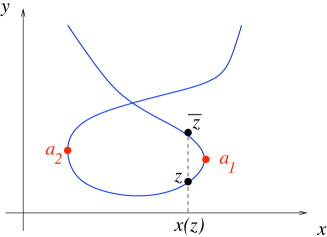
z¯¯𝑧\bar{z} is called the conjugate point to z𝑧z, and it is defined only in the vicinity of branch points, as depicted in figure 6.

We also require that the branch points of x𝑥x and y𝑦y do not coincide, such that dy(ai)0𝑑𝑦subscript𝑎𝑖0dy(a_{i})\neq 0 and y(z)𝑦𝑧y(z) therefore has a square-root branchcut as a function of x𝑥x at x(ai)𝑥subscript𝑎𝑖x(a_{i}). If y𝑦y is finite at aisubscript𝑎𝑖a_{i}, its local behavior is hence given by

y(z)y(ai)+Cix(z)x(ai).similar-to𝑦𝑧𝑦subscript𝑎𝑖subscript𝐶𝑖𝑥𝑧𝑥subscript𝑎𝑖y(z)\sim y(a_{i})+C_{i}\sqrt{x(z)-x(a_{i})}\,.

If aisubscript𝑎𝑖a_{i} corresponds to a hard edge, we require y𝑦y to have a pole here. Its local behavior is hence given by
y(z)Cix(z)x(ai).similar-to𝑦𝑧subscript𝐶𝑖𝑥𝑧𝑥subscript𝑎𝑖y(z)\sim{C_{i}\over\sqrt{x(z)-x(a_{i})}}\,.
Refer to caption
Figure 6: At a regular branch point a𝒞𝑎𝒞a\in{{\mathcal{C}}} of x𝑥x, y𝑦y as a function of x𝑥x has a branchcut yy(a)+Cxx(a)similar-to𝑦𝑦𝑎𝐶𝑥𝑥𝑎y\sim y(a)+C\sqrt{x-x(a)}. If z𝑧z is a point on one branch near a𝑎a, we call z¯¯𝑧\bar{z} the conjugate point on the other branch; it has the same x𝑥x projection, x(z¯)=x(z)𝑥¯𝑧𝑥𝑧x(\bar{z})=x(z). Notice that z¯¯𝑧\bar{z} is defined only locally near branch points. If we follow z𝑧z from a1subscript𝑎1a_{1} to a2subscript𝑎2a_{2}, z¯¯𝑧\bar{z} may have to jump from one branch to another.

4.3.2 Bergman kernel

On a curve 𝒞𝒞{{\mathcal{C}}}, there exists a unique symmetric 2-form B(z1,z2)𝐵subscript𝑧1subscript𝑧2B(z_{1},z_{2}) with a double pole on the diagonal z1=z2subscript𝑧1subscript𝑧2z_{1}=z_{2} and no other poles, with the following normalization on 𝒜𝒜{\cal A}-cycles,

z2𝒜j,iB(z1,z2)=0.subscriptcontour-integralsubscript𝑧2subscript𝒜𝑗𝑖𝐵subscript𝑧1subscript𝑧20\oint_{z_{2}\in{\cal A}_{j,i}}B(z_{1},z_{2})=0.

In any local coordinate near z1=z2subscript𝑧1subscript𝑧2z_{1}=z_{2}, one has

B(z1,z2)dz1dz2(z1z2)2+regular.similar-to𝐵subscript𝑧1subscript𝑧2𝑑subscript𝑧1𝑑subscript𝑧2superscriptsubscript𝑧1subscript𝑧22regularB(z_{1},z_{2})\sim{dz_{1}\,dz_{2}\over(z_{1}-z_{2})^{2}}+{\rm regular}\,.

B𝐵B is called the Bergman kernel of 𝒞𝒞{{\mathcal{C}}}, or the fundamental 2-form of the second kind [34].

4.3.3 Recursion kernel

We now define the recursion kernel K𝐾K as

K(z0,z)=z¯zB(z0,z)2(y(z¯)y(z))dx(z).𝐾subscript𝑧0𝑧superscriptsubscript¯𝑧𝑧𝐵subscript𝑧0superscript𝑧2𝑦¯𝑧𝑦𝑧𝑑𝑥𝑧K(z_{0},z)=\frac{\int_{\bar{z}}^{z}B(z_{0},z^{\prime})}{2(y(\bar{z})-y(z))\,dx(z)}\,.

This kernel is a globally defined 1-form in the variable z0𝒞subscript𝑧0𝒞z_{0}\in{{\mathcal{C}}}. In the variable z𝑧z, it is the inverse of a 1-form (that means we have to multiply it with a quadratic differential before computing any integral with it); it is defined only locally near branch points of x𝑥x, such that K(z0,z¯)=K(z0,z)𝐾subscript𝑧0¯𝑧𝐾subscript𝑧0𝑧K(z_{0},\bar{z})=K(z_{0},z). At the branch points, it has simple poles,

K(z0,z)B(z0,z)2dx(z)dy(z)+regular.similar-to𝐾subscript𝑧0𝑧𝐵subscript𝑧0𝑧2𝑑𝑥𝑧𝑑𝑦𝑧regularK(z_{0},z)\sim-{B(z_{0},z)\over 2\,dx(z)\,dy(z)}+{\rm regular}.

4.3.4 Topological recursion

Correlation forms Wn(g)(z1,,zn)superscriptsubscript𝑊𝑛𝑔subscript𝑧1subscript𝑧𝑛W_{n}^{(g)}(z_{1},\ldots,z_{n}) (not to be confused with the resolvents Wi(z)subscript𝑊𝑖𝑧W_{i}(z) introduced above) are symmetric n𝑛n-forms defined by

W1(0)(z)=y(z)dx(z),superscriptsubscript𝑊10𝑧𝑦𝑧𝑑𝑥𝑧W_{1}^{(0)}(z)=-y(z)dx(z)\,,
W2(0)(z1,z2)=B(z1,z2),superscriptsubscript𝑊20subscript𝑧1subscript𝑧2𝐵subscript𝑧1subscript𝑧2W_{2}^{(0)}(z_{1},z_{2})=B(z_{1},z_{2})\,,

and then by recursion (we write collectively J={z1,,zn}𝐽subscript𝑧1subscript𝑧𝑛J=\{z_{1},\dots,z_{n}\}),

Wn+1(g)(z0,J)superscriptsubscript𝑊𝑛1𝑔subscript𝑧0𝐽\displaystyle W_{n+1}^{(g)}(z_{0},J) =\displaystyle= iReszaiK(z0,z)[Wn+2(g1)(z,z¯,J)\displaystyle\sum_{i}\mathop{{\rm Res}\,}_{z\to a_{i}}K(z_{0},z)\,\Big{[}W_{n+2}^{(g-1)}(z,\bar{z},J)
+h=0gIJW1+|I|(h)(z,I)W1+n|I|(gh)(z¯,JI)]\displaystyle+\sum_{h=0}^{g}\sum^{\prime}_{I\subset J}W_{1+|I|}^{(h)}(z,I)\,W_{1+n-|I|}^{(g-h)}(\bar{z},J\setminus I)\Big{]}

where Isubscriptsuperscript𝐼\sum^{\prime}_{I} is the sum over all subsets of J𝐽J, restricted to (h,I)(0,)𝐼0(h,I)\neq(0,\emptyset) and (h,I)(g,J)𝐼𝑔𝐽(h,I)\neq(g,J).

Although it is not obvious from the definition, the forms Wn(g)superscriptsubscript𝑊𝑛𝑔W_{n}^{(g)} are symmetric. For 22gn<022𝑔𝑛02-2g-n<0, they are meromorphic n𝑛n-forms with poles only at branch points. These poles are of degree at most 6g4+2n6𝑔42𝑛6g-4+2n, and have vanishing residues.

For the one matrix model, the Wn(g)superscriptsubscript𝑊𝑛𝑔W_{n}^{(g)} coincide with the n𝑛n-point function of the trace of the resolvent at order g𝑔g in the topological expansion.

4.3.5 Symplectic invariants

Finally, for g2𝑔2g\geq 2, we define the symplectic invariants Fgsubscript𝐹𝑔F_{g} (also denoted W0(g)subscript𝑊0𝑔W_{0}(g) in [3]) by

Fg(𝒮)=122giReszaiΦ(z)W1(g)(z),subscript𝐹𝑔𝒮122𝑔subscript𝑖subscriptRes𝑧subscript𝑎𝑖Φ𝑧superscriptsubscript𝑊1𝑔𝑧F_{g}({{\mathcal{S}}})={1\over 2-2g}\,\sum_{i}\mathop{{\rm Res}\,}_{z\to a_{i}}\Phi(z)\,W_{1}^{(g)}(z)\,,

where ΦΦ\Phi is any function defined locally near branch points of x𝑥x such that dΦ=ydx𝑑Φ𝑦𝑑𝑥d\Phi=ydx.

The definitions of F1subscript𝐹1F_{1} and F0subscript𝐹0F_{0} are more involved and we refer the reader to [3]. F0subscript𝐹0F_{0} is called the prepotential, and F1subscript𝐹1F_{1} is closely related to the determinant of the Laplacian on 𝒞𝒞{{\mathcal{C}}} with metrics |ydx|2superscript𝑦𝑑𝑥2|ydx|^{2}, see [35, 36].

The Fg(𝒮)subscript𝐹𝑔𝒮F_{g}({{\mathcal{S}}})’s depend only on the orbit of 𝒮𝒮{{\mathcal{S}}} under the group of transformations generated by

  • ::absent\mathfrak{R}:

    𝒮𝒮~=(𝒞,x,y+R(x))maps-to𝒮~𝒮𝒞𝑥𝑦𝑅𝑥{{\mathcal{S}}}\mapsto\tilde{{\mathcal{S}}}=({{\mathcal{C}}},x,y+R(x)) where R(x)𝑅𝑥R(x) is any rational function of x𝑥x,

  • 𝔉::𝔉absent\mathfrak{F}:

    𝒮𝒮~=(𝒞,f(x),y/f(x))maps-to𝒮~𝒮𝒞𝑓𝑥𝑦superscript𝑓𝑥{{\mathcal{S}}}\mapsto\tilde{{\mathcal{S}}}=({{\mathcal{C}}},f(x),y/f^{\prime}(x)) where f(x)𝑓𝑥f(x) is an analytical function of x𝑥x, with fsuperscript𝑓f^{\prime} rational, such that df=fdx𝑑𝑓superscript𝑓𝑑𝑥df=f^{\prime}dx has the same number of zeroes as dx𝑑𝑥dx,

  • 𝔖::𝔖absent\mathfrak{S}:

    𝒮𝒮~=(𝒞,y,x)maps-to𝒮~𝒮𝒞𝑦𝑥{{\mathcal{S}}}\mapsto\tilde{{\mathcal{S}}}=({{\mathcal{C}}},y,-x).

These transformations are symplectic, i.e. they leave dxdy𝑑𝑥𝑑𝑦dx\wedge dy invariant.

The symplectic invariants are homogeneous of degree 22g22𝑔2-2g,

Fg(𝒞,x,λy)=λ22gFg(𝒞,x,y).subscript𝐹𝑔𝒞𝑥𝜆𝑦superscript𝜆22𝑔subscript𝐹𝑔𝒞𝑥𝑦F_{g}({{\mathcal{C}}},x,\lambda y)=\lambda^{2-2g}\,F_{g}({{\mathcal{C}}},x,y). (4.8)

In particular, they are invariant under the parity transformation Fg(𝒞,x,y)=Fg(𝒞,x,y)subscript𝐹𝑔𝒞𝑥𝑦subscript𝐹𝑔𝒞𝑥𝑦F_{g}({{\mathcal{C}}},x,-y)=F_{g}({{\mathcal{C}}},x,y).

5 The spectral curve for the topological string’s matrix model

Applying the procedure outlined in section 4.2.2 to our matrix model, we will determine a spectral curve 𝒮MM(𝔛0)subscript𝒮𝑀𝑀subscript𝔛0{{\mathcal{S}}}_{MM}({\mathfrak{X}}_{0}) in this section. [27] demonstrated that for a chain of matrices, we have

lnZ=ggs2g2Fg(𝒮MM),𝑍subscript𝑔superscriptsubscript𝑔𝑠2𝑔2subscript𝐹𝑔subscript𝒮MM\ln{Z}=\sum_{g}g_{s}^{2g-2}F_{g}({{\mathcal{S}}_{\rm MM}})\,,

with Fgsubscript𝐹𝑔F_{g} the symplectic invariants of [3]. In our case, since we have engineered our matrix model to yield555As we have here reserved the notation Fgsubscript𝐹𝑔F_{g} for the symplectic invariants of our matrix model, we refer to the topological string free energies as GWg𝐺subscript𝑊𝑔GW_{g}. GWg(𝔛0)𝐺subscript𝑊𝑔subscript𝔛0GW_{g}({\mathfrak{X}}_{0}) as its partition function, re-computing the partition function via the methods of [27] will yield

GWg(𝔛0)=Fg(𝒮MM).𝐺subscript𝑊𝑔subscript𝔛0subscript𝐹𝑔subscript𝒮MMGW_{g}({\mathfrak{X}}_{0})=F_{g}({{\mathcal{S}}_{\rm MM}})\,.

This relation is already quite interesting, as it allows for explicit computation of the Gromov-Witten invariants. Our goal however will be to go further. We will argue that 𝒮MMsubscript𝒮MM{{\mathcal{S}}_{\rm MM}} is symplectically equivalent to the mirror spectral curve 𝒮𝔛^0subscript𝒮subscript^𝔛0{{\mathcal{S}}}_{\hat{\mathfrak{X}}_{0}} of section 2.2,

𝒮MM𝒮𝔛0.similar-tosubscript𝒮MMsubscript𝒮subscript𝔛0{{\mathcal{S}}_{\rm MM}}\sim{{\mathcal{S}}}_{{\mathfrak{X}}_{0}}\,.

Since the Fgsubscript𝐹𝑔F_{g}’s are symplectic invariants, this will imply the BKMP conjecture for 𝔛0subscript𝔛0{\mathfrak{X}}_{0}, i.e.

GWg(𝔛0)=Fg(𝒮𝔛0).𝐺subscript𝑊𝑔subscript𝔛0subscript𝐹𝑔subscript𝒮subscript𝔛0GW_{g}({\mathfrak{X}}_{0})=F_{g}({{\mathcal{S}}}_{{\mathfrak{X}}_{0}}).

5.1 Applying the chain of matrices rules

We now apply the rules of section 4.2.2 to the chain of matrices model introduced in section 3.

  • Recall that the integration ensembles for the matrices M0subscript𝑀0M_{0} and Mm+1subscript𝑀𝑚1M_{m+1} are such that for each matrix, all eigenvalues are integrated on the same contour (A.7). Hence, k0=km+1=1subscript𝑘0subscript𝑘𝑚11k_{0}=k_{m+1}=1, and the corresponding filling fractions are equal to N𝑁N. For i=1,,m𝑖1𝑚i=1,\dots,m, the matrix Misubscript𝑀𝑖M_{i} is integrated on H(γ0,id×γ2,id××γn,id)𝐻superscriptsubscript𝛾0𝑖𝑑superscriptsubscript𝛾2𝑖𝑑superscriptsubscript𝛾𝑛𝑖𝑑H(\gamma_{0,i}^{d}\times\gamma_{2,i}^{d}\times\dots\times\gamma_{n,i}^{d}), where γj,isubscript𝛾𝑗𝑖\gamma_{j,i} is a contour which surrounds all points of the form qaj,i+superscript𝑞subscript𝑎𝑗𝑖q^{a_{j,i}+\mathbb{N}}. There are thus ki=n+1subscript𝑘𝑖𝑛1k_{i}=n+1 filling fractions, each equal to d𝑑d. The matrices Risubscript𝑅𝑖R_{i} are integrated on H(+N)𝐻superscriptsubscript𝑁H(\mathbb{R}_{+}^{N}). We denote the number of their cuts by ki~~subscript𝑘𝑖\tilde{k_{i}}. Hence, k~i=1subscript~𝑘𝑖1\tilde{k}_{i}=1, with the respective filling fraction equal to N𝑁N.

    According to condition 1 of section 4.2.2, the genus of the spectral curve 𝒞𝒞{{\mathcal{C}}} is thus given by

    𝔤=i=0m+1(ki1)+i=1m+1(k~i1)=nm.𝔤superscriptsubscript𝑖0𝑚1subscript𝑘𝑖1superscriptsubscript𝑖1𝑚1subscript~𝑘𝑖1𝑛𝑚\mathfrak{g}=\sum_{i=0}^{m+1}(k_{i}-1)+\sum_{i=1}^{m+1}(\tilde{k}_{i}-1)=nm\,.
  • Following condition 2 of section 4.2.2, we introduce functions xi(z)subscript𝑥𝑖𝑧x_{i}(z), i=0,,m+1𝑖0𝑚1i=0,\dots,m+1, associated to the matrices Misubscript𝑀𝑖M_{i}, and functions yi(z)subscript𝑦𝑖𝑧y_{i}(z), i=1,,m+1𝑖1𝑚1i=1,\dots,m+1, associated to the matrices Risubscript𝑅𝑖R_{i}, as well as two additional functions y0(z)subscript𝑦0𝑧y_{0}(z) and ym+2(z)subscript𝑦𝑚2𝑧y_{m+2}(z) at the ends of the chain.

    They must satisfy the following requirements:

    • Since there is no potential for the matrices Risubscript𝑅𝑖R_{i}, equation (4.4) implies that we have, for i=1,,m+1𝑖1𝑚1i=1,\dots,m+1,

      xi(z)xi1(z)=0.subscript𝑥𝑖𝑧subscript𝑥𝑖1𝑧0x_{i}(z)-x_{i-1}(z)=0\,.

      We can hence suppress the index i𝑖i on these functions, x(z)=xi(z)𝑥𝑧subscript𝑥𝑖𝑧x(z)=x_{i}(z).

    • For i=1,,m𝑖1𝑚i=1,\dots,m, equation (4.4) gives

      yi(z)yi+1(z)=2Vai(x(z))Vai+1(x(z))Vai1(x(z))gsfi(x(z))fi(x(z))gsSi+iπx(z)subscript𝑦𝑖𝑧subscript𝑦𝑖1𝑧2subscriptsuperscript𝑉subscript𝑎𝑖𝑥𝑧subscriptsuperscript𝑉subscript𝑎𝑖1𝑥𝑧subscriptsuperscript𝑉subscript𝑎𝑖1𝑥𝑧subscript𝑔𝑠subscriptsuperscript𝑓𝑖𝑥𝑧subscript𝑓𝑖𝑥𝑧subscript𝑔𝑠subscript𝑆𝑖𝑖𝜋𝑥𝑧y_{i}(z)-y_{i+1}(z)=2V^{\prime}_{\vec{a}_{i}}(x(z))-V^{\prime}_{\vec{a}_{i+1}}(x(z))-V^{\prime}_{\vec{a}_{i-1}}(x(z))-g_{s}{f^{\prime}_{i}(x(z))\over f_{i}(x(z))}-{g_{s}\,S_{i}+i\pi\over x(z)}

      and

      y0(z)y1(z)=Va0(x(z))Va1(x(z))gsf0(x(z))f0(x(z)),subscript𝑦0𝑧subscript𝑦1𝑧subscriptsuperscript𝑉subscript𝑎0𝑥𝑧subscriptsuperscript𝑉subscript𝑎1𝑥𝑧subscript𝑔𝑠subscriptsuperscript𝑓0𝑥𝑧subscript𝑓0𝑥𝑧y_{0}(z)-y_{1}(z)=V^{\prime}_{\vec{a}_{0}}(x(z))-V^{\prime}_{\vec{a}_{1}}(x(z))-g_{s}{f^{\prime}_{0}(x(z))\over f_{0}(x(z))}\,,
      ym+1(z)ym+2(z)=Vam+1(x(z))Vam(x(z))gsfm+1(x(z))fm+1(x(z)).subscript𝑦𝑚1𝑧subscript𝑦𝑚2𝑧subscriptsuperscript𝑉subscript𝑎𝑚1𝑥𝑧subscriptsuperscript𝑉subscript𝑎𝑚𝑥𝑧subscript𝑔𝑠subscriptsuperscript𝑓𝑚1𝑥𝑧subscript𝑓𝑚1𝑥𝑧y_{m+1}(z)-y_{m+2}(z)=V^{\prime}_{\vec{a}_{m+1}}(x(z))-V^{\prime}_{\vec{a}_{m}}(x(z))-g_{s}{f^{\prime}_{m+1}(x(z))\over f_{m+1}(x(z))}\,.

      More explicitly, in terms of the function

      ψq(x)=xg(x)/g(x),subscript𝜓𝑞𝑥𝑥superscript𝑔𝑥𝑔𝑥\psi_{q}(x)=xg^{\prime}(x)/g(x)\,,

      whose small gssubscript𝑔𝑠g_{s} expansion

      ψq(x)subscript𝜓𝑞𝑥\displaystyle\psi_{q}(x) =\displaystyle= 1lnqn=0(1)nBnn!(lnq)nLi1n(1/x)1𝑞superscriptsubscript𝑛0superscript1𝑛subscript𝐵𝑛𝑛superscript𝑞𝑛subscriptLi1n1x\displaystyle-\,{1\over\ln q}\,\sum_{n=0}^{\infty}{(-1)^{n}\,B_{n}\over n!}\,(\ln q)^{n}\,\,\rm Li_{1-n}(1/x)
      =\displaystyle= 1lnq[ln(11x)lnq2(x1)n=1B2n(2n)!(lnq)2nLi12n(x)].1𝑞delimited-[]11𝑥𝑞2𝑥1superscriptsubscript𝑛1subscript𝐵2𝑛2𝑛superscript𝑞2𝑛subscriptLi12nx\displaystyle{1\over\ln{q}}\,\Big{[}\ln{(1-{1\over x})}-{\ln q\over 2(x-1)}-\sum_{n=1}^{\infty}{B_{2n}\over(2n)!}\,\,(\ln q)^{2n}\,\rm Li_{1-2n}(x)\Big{]}\,.

      we worked out in appendix A of [1], we obtain

      x(z)(yi+1(z)yi(z))𝑥𝑧subscript𝑦𝑖1𝑧subscript𝑦𝑖𝑧\displaystyle x(z)(y_{i+1}(z)-y_{i}(z)) (5.1)
      =\displaystyle= iπ+gsSigsj(2ψq(qaj,i/x(z))ψq(qaj,i+1/x(z))ψq(qaj,i1/x(z)))𝑖𝜋subscript𝑔𝑠subscript𝑆𝑖subscript𝑔𝑠subscript𝑗2subscript𝜓𝑞superscript𝑞subscript𝑎𝑗𝑖𝑥𝑧subscript𝜓𝑞superscript𝑞subscript𝑎𝑗𝑖1𝑥𝑧subscript𝜓𝑞superscript𝑞subscript𝑎𝑗𝑖1𝑥𝑧\displaystyle i\pi+g_{s}S_{i}-g_{s}\sum_{j}(2\psi_{q}(q^{a_{j,i}}/x(z))-\psi_{q}(q^{a_{j,i+1}}/x(z))-\psi_{q}(q^{a_{j,i-1}}/x(z)))
      +gsx(z)fi(x(z))fi(x(z)),subscript𝑔𝑠𝑥𝑧subscriptsuperscript𝑓𝑖𝑥𝑧subscript𝑓𝑖𝑥𝑧\displaystyle+g_{s}{x(z)f^{\prime}_{i}(x(z))\over f_{i}(x(z))}\,,

      as well as

      x(z)(y1(z)y0(z))𝑥𝑧subscript𝑦1𝑧subscript𝑦0𝑧\displaystyle x(z)(y_{1}(z)-y_{0}(z)) =\displaystyle= gsjψq(qaj,0/x(z))+gsjψq(qaj,1/x(z))subscript𝑔𝑠subscript𝑗subscript𝜓𝑞superscript𝑞subscript𝑎𝑗0𝑥𝑧subscript𝑔𝑠subscript𝑗subscript𝜓𝑞superscript𝑞subscript𝑎𝑗1𝑥𝑧\displaystyle-g_{s}\sum_{j}\psi_{q}(q^{a_{j,0}}/x(z))+g_{s}\sum_{j}\psi_{q}(q^{a_{j,1}}/x(z))
      gsjk=0d1x(z)x(z)qaj,0+k,subscript𝑔𝑠subscript𝑗superscriptsubscript𝑘0𝑑1𝑥𝑧𝑥𝑧superscript𝑞subscript𝑎𝑗0𝑘\displaystyle-g_{s}\sum_{j}\sum_{k=0}^{d-1}\frac{x(z)}{x(z)-q^{a_{j,0}+k}}\,,
      x(z)(ym+2(z)ym+1(z))𝑥𝑧subscript𝑦𝑚2𝑧subscript𝑦𝑚1𝑧\displaystyle x(z)(y_{m+2}(z)-y_{m+1}(z)) =\displaystyle= gsjψq(qaj,m+1/x(z))+gsjψq(qaj,m/x(z))subscript𝑔𝑠subscript𝑗subscript𝜓𝑞superscript𝑞subscript𝑎𝑗𝑚1𝑥𝑧subscript𝑔𝑠subscript𝑗subscript𝜓𝑞superscript𝑞subscript𝑎𝑗𝑚𝑥𝑧\displaystyle-g_{s}\sum_{j}\psi_{q}(q^{a_{j,m+1}}/x(z))+g_{s}\sum_{j}\psi_{q}(q^{a_{j,m}}/x(z))
      gsjk=0d1x(z)x(z)qaj,m+1+ksubscript𝑔𝑠subscript𝑗superscriptsubscript𝑘0𝑑1𝑥𝑧𝑥𝑧superscript𝑞subscript𝑎𝑗𝑚1𝑘\displaystyle-g_{s}\sum_{j}\sum_{k=0}^{d-1}\frac{x(z)}{x(z)-q^{a_{j,m+1}+k}}

      Note that we have explicitly used the fact that the partitions αj,m+1subscript𝛼𝑗𝑚1\alpha_{j,m+1} and αj,0subscript𝛼𝑗0\alpha_{j,0} are chosen to be trivial.

    • Since the integral over Risubscript𝑅𝑖R_{i} is over HN(+)subscript𝐻𝑁subscriptH_{N}(\mathbb{R}_{+}), i.e. its eigenvalues are integrated on +subscript\mathbb{R}_{+}, the integration contour has an endpoint (hard edge) at yi=0subscript𝑦𝑖0y_{i}=0. Condition 3 hence requires that at a pre-image yi1(0)superscriptsubscript𝑦𝑖10y_{i}^{-1}(0), which we will refer to as isubscript𝑖\infty_{i}, the following holds

      yi(i)=0,dyi(i)=0,x(z)hasasimplepoleatz=i.formulae-sequencesubscript𝑦𝑖subscript𝑖0formulae-sequence𝑑subscript𝑦𝑖subscript𝑖0𝑥𝑧hasasimplepoleat𝑧subscript𝑖y_{i}(\infty_{i})=0\,,\quad dy_{i}(\infty_{i})=0\,,\quad x(z){\rm\,\,has\,a\,simple\,pole\,at\,}z=\infty_{i}\,.

      Furthermore, introducing a local parameter z𝑧z in the neighborhood of isubscript𝑖\infty_{i}, the above translates into

      yi(z)z2,x(z)1/z.formulae-sequencesimilar-tosubscript𝑦𝑖𝑧superscript𝑧2similar-to𝑥𝑧1𝑧y_{i}(z)\sim z^{2}\,,\quad x(z)\sim 1/z\,.

      Hence, i=1,,m+1for-all𝑖1𝑚1\forall\,i=1,\dots,m+1,

      yi𝒪(1/x2).similar-tosubscript𝑦𝑖𝒪1superscript𝑥2y_{i}\sim{\cal O}(1/x^{2})\,.
  • The relations (5.1) imply that near isubscript𝑖\infty_{i}, we have

    x(yj+1yj)ziiπ+gsSj+gsl=0n(2al,jal,j+1al,j1)+O(1/x).𝑥subscript𝑦𝑗1subscript𝑦𝑗subscriptsimilar-to𝑧subscript𝑖𝑖𝜋subscript𝑔𝑠subscript𝑆𝑗subscript𝑔𝑠superscriptsubscript𝑙0𝑛2subscript𝑎𝑙𝑗subscript𝑎𝑙𝑗1subscript𝑎𝑙𝑗1𝑂1𝑥x(y_{j+1}-y_{j})\mathop{{\sim}}_{z\to\infty_{i}}i\pi+g_{s}S_{j}+g_{s}\sum_{l=0}^{n}(2a_{l,j}-a_{l,j+1}-a_{l,j-1})+O(1/x)\,.

    In particular, it follows that jisubscript𝑗subscript𝑖\infty_{j}\neq\infty_{i}. Thus, all points {1,,m+1}x1()subscript1subscript𝑚1superscript𝑥1\{\infty_{1},\dots,\infty_{m+1}\}\subset x^{-1}(\infty) are distinct , i.e. condition 3 requires that x1()superscript𝑥1x^{-1}(\infty) have at least m+1𝑚1m+1 points.

    We will make the minimal assumption that x1()superscript𝑥1x^{-1}(\infty) has exactly m+1𝑚1m+1 elements that are simple poles of x𝑥x, and that x𝑥x has no further singularities, i.e. that x𝑥x is a meromorphic function of degree m+1𝑚1m+1 on 𝒞𝒞{{\mathcal{C}}}.

  • By condition 5, since for i=0,,m+2𝑖0𝑚2i=0,\dots,m+2 there are d𝑑d eigenvalues of Misubscript𝑀𝑖M_{i} of the form qaj,i+superscript𝑞subscript𝑎𝑗𝑖q^{a_{j,i}+\mathbb{N}} surrounded by the path 𝒜^j,isubscript^𝒜𝑗𝑖\widehat{\cal A}_{j,i} , we have the (m+2)×(n+1)𝑚2𝑛1(m+2)\times(n+1) filling fraction conditions

    12iπ𝒜j,iyi𝑑x=dgsfori=0,,m+1,j=0,,n.formulae-sequence12𝑖𝜋subscriptcontour-integralsubscript𝒜𝑗𝑖subscript𝑦𝑖differential-d𝑥𝑑subscript𝑔𝑠formulae-sequencefor𝑖0𝑚1𝑗0𝑛{1\over 2i\pi}\oint_{{\cal A}_{j,i}}y_{i}\,dx=d\,g_{s}\qquad\mathrm{for}\,\,i=0,\dots,m+1,\,\,\,j=0,\dots,n\,.
Refer to caption
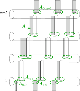
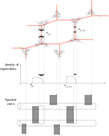
Figure 7: The spectral curve of our matrix model can be represented as follows. The cover of 1superscript1\mathbb{C}\mathbb{P}^{1} provided by x𝑥x has m+1𝑚1m+1 sheets. Instead of the projective plane of x𝑥x, we represent the sheets of lnx𝑥\ln x, which are cylinders. Cycles 𝒜j,isubscript𝒜𝑗𝑖{\cal A}_{j,i} appear in sheets i1𝑖1i-1 and i𝑖i. They enclose singularities of the resolvent Wisubscript𝑊𝑖W_{i}. Algebraic cuts are represented as vertical cylinders, and poles and log singularities are represented as grey strips. There is only one cycle 𝒜j,0subscript𝒜𝑗0{\cal A}_{j,0} (which is in sheet 00) and one 𝒜j,m+1subscript𝒜𝑗𝑚1{\cal A}_{j,m+1} (in sheet m𝑚m), and they enclose only poles or log singularities of y0subscript𝑦0y_{0} resp. ym+1subscript𝑦𝑚1y_{m+1}.

x𝑥x hence defines an m+1𝑚1m+1 sheeted cover of 1superscript1\mathbb{C}\mathbb{P}^{1}. Considering the function lnx𝑥\ln x instead, with singularities at x=0𝑥0x=0 and x=𝑥x=\infty, each sheet of this cover is mapped to a cylinder. We have depicted this covering in figure 7, and indicated the singularities of yisubscript𝑦𝑖y_{i} on each sheet: algebraic cuts are represented by vertical cylinders, and poles and logarithmic cuts by grey strips.

In sheet i𝑖i we have represented some contours 𝒜j,isubscript𝒜𝑗𝑖{\cal A}_{j,i} whose image under the projection x:𝒞1:𝑥𝒞superscript1x:{{\mathcal{C}}}\to\mathbb{C}\mathbb{P}^{1} surrounds all points of type qaj,i+superscript𝑞subscript𝑎𝑗𝑖q^{a_{j,i}+\mathbb{N}}.

For i=1,,m𝑖1𝑚i=1,\dots,m, the resolvent Wi(x)subscript𝑊𝑖𝑥W_{i}(x) of the ithsuperscript𝑖thi^{\rm th} matrix Misubscript𝑀𝑖M_{i} is computed as a contour integral around the sum over j𝑗j of cycles 𝒜j,isubscript𝒜𝑗𝑖{\cal A}_{j,i} on sheet i𝑖i,

Wi(x)=j=0n12iπ𝒜j,iyi(z)dx(z)xx(z).subscript𝑊𝑖𝑥superscriptsubscript𝑗0𝑛12𝑖𝜋subscriptcontour-integralsubscript𝒜𝑗𝑖subscript𝑦𝑖superscript𝑧𝑑𝑥superscript𝑧𝑥𝑥superscript𝑧W_{i}(x)=\sum_{j=0}^{n}\,{1\over 2i\pi}\oint_{{\cal A}_{j,i}}\,{y_{i}(z^{\prime})dx(z^{\prime})\over x-x(z^{\prime})}\,.

Also, as argued in [1], the potentials of M0subscript𝑀0M_{0} and Mm+1subscript𝑀𝑚1M_{m+1} are such that in fact the matrices M0subscript𝑀0M_{0} and Mm+1subscript𝑀𝑚1M_{m+1} are frozen, and thus their resolvents contain only poles. In terms of the functions y0subscript𝑦0y_{0} and ym+1subscript𝑦𝑚1y_{m+1}, we conclude that the singularities of y0subscript𝑦0y_{0} in 𝒜j,0subscript𝒜𝑗0{\cal A}_{j,0} in sheet 111 and the singularities of ym+1subscript𝑦𝑚1y_{m+1} in 𝒜j,m+1subscript𝒜𝑗𝑚1{\cal A}_{j,m+1} in sheet m+1𝑚1m+1 can be only poles, not cuts.

Since condition 1 requires that the genus be 𝔤=nm𝔤𝑛𝑚\mathfrak{g}=nm, we see that there can be no other cuts than the ones already discussed – the genus would be higher, otherwise.

5.2 Symplectic change of functions

The spectral curve of the matrix model is 𝒮MM=(𝒞,x,y0)subscript𝒮𝑀𝑀𝒞𝑥subscript𝑦0{{\mathcal{S}}}_{MM}=({{\mathcal{C}}},x,y_{0}), and our goal is to relate it to the mirror curve described in section 2.2. The mirror curve is described via the algebraic equation (2.3) in the two functions x1,x2:𝒞mirror1:subscript𝑥1subscript𝑥2subscript𝒞𝑚𝑖𝑟𝑟𝑜𝑟superscript1x_{1},x_{2}:{{\mathcal{C}}}_{mirror}\rightarrow\mathbb{C}\mathbb{P}^{1} (in the patch x0=1subscript𝑥01x_{0}=1). We wish to obtain a similar algebraic description of 𝒞𝒞{{\mathcal{C}}}. Due to log singularities in y0subscript𝑦0y_{0}, to be traced to the small gssubscript𝑔𝑠g_{s} behavior of ψq(x)subscript𝜓𝑞𝑥\psi_{q}(x), an algebraic equation in the variables (x,y0)𝑥subscript𝑦0(x,y_{0}) cannot exist (recall that x𝑥x is meromorphic). In this section, we shall, via a series of symplectic transformations on the yisubscript𝑦𝑖y_{i} of the type enumerated in section 4.3.5, arrive at functions Yisubscript𝑌𝑖Y_{i} that are meromorphic on 𝒞𝒞{{\mathcal{C}}}, and hence each present a viable candidate to pair with x𝑥x to yield an algebraic equation for 𝒞𝒞{{\mathcal{C}}}.


Essentially, we wish to introduce the exponentials of yisubscript𝑦𝑖y_{i}. While this will eliminate the log singularities, poles in yisubscript𝑦𝑖y_{i} would be elevated to essential singularities. We hence first turn to the question of eliminating these poles.

5.2.1 The arctic circle property

On the physical sheet, the interpretation of a pole of yisubscript𝑦𝑖y_{i} is as an eigenvalue of the matrix Misubscript𝑀𝑖M_{i} with delta function support. Such a so-called frozen eigenvalue can arise in the following way:

The sum over all partitions is dominated by partitions close to a typical equilibrium partition, i.e. a saddle point. The typical partition has a certain typical length referred to as its equilibrium length n¯¯𝑛\bar{n}. All partitions with a length very different from the equilibrium length contribute only in an exponentially small way (and thus non-perturbatively) to the full partition function. Introducing a cutoff on the length of partitions which is larger than the equilibrium length hence does not change the perturbative part of the partition function. Now recall that when we defined the hi(γ)subscript𝑖𝛾h_{i}(\gamma) of a representation γ𝛾\gamma in appendix A, we introduced an arbitrary maximal length d𝑑d such that l(γ)d𝑙𝛾𝑑l(\gamma)\leq d and set

hi(γ)=aγ+di+γi.subscript𝑖𝛾subscript𝑎𝛾𝑑𝑖subscript𝛾𝑖h_{i}(\gamma)=a_{\gamma}+d-i+\gamma_{i}\,.

Setting γi=0subscript𝛾𝑖0\gamma_{i}=0 for di>n¯𝑑𝑖¯𝑛d\geq i>\bar{n} yields hisubscript𝑖h_{i} that do not depend on the integration variables, hence are frozen at fixed values. This behavior is referred to as the arctic circle property [37], as all eigenvalues beyond the arctic circle situated at equilibrium length n¯¯𝑛\bar{n} are frozen.

Returning to our matrix model, the eigenvalues of the matrices Misubscript𝑀𝑖M_{i} are given by q(hj,i)lsuperscript𝑞subscriptsubscript𝑗𝑖𝑙q^{(h_{j,i})_{l}}. For dl>nj,i𝑑𝑙subscript𝑛𝑗𝑖d\geq l>n_{j,i}, they are frozen, and thus contribute poles to yisubscript𝑦𝑖y_{i} by (4.5) (recall that poles of the resolvent correspond to eigenvalues with delta function support) in the physical sheet. We will assume that these are the only poles in the physical sheet and we subtract them to obtain new functions y~isubscript~𝑦𝑖\tilde{y}_{i},

y~0(z)=x(z)y0(z)jk=0d1gsx(z)x(z)qaj,0+k,subscript~𝑦0𝑧𝑥𝑧subscript𝑦0𝑧subscript𝑗superscriptsubscript𝑘0𝑑1subscript𝑔𝑠𝑥𝑧𝑥𝑧superscript𝑞subscript𝑎𝑗0𝑘\displaystyle\tilde{y}_{0}(z)=x(z)y_{0}(z)-\sum_{j}\sum_{k=0}^{d-1}{g_{s}x(z)\over x(z)-q^{a_{j,0}+k}}\,,
y~m+2(z)=x(z)ym+2(z)+j0d1gsx(z)x(z)qaj,m+1+ksubscript~𝑦𝑚2𝑧𝑥𝑧subscript𝑦𝑚2𝑧subscript𝑗superscriptsubscript0𝑑1subscript𝑔𝑠𝑥𝑧𝑥𝑧superscript𝑞subscript𝑎𝑗𝑚1𝑘\displaystyle\tilde{y}_{m+2}(z)=x(z)y_{m+2}(z)+\sum_{j}\sum_{0}^{d-1}{g_{s}x(z)\over x(z)-q^{a_{j,m+1}+k}}

and for i=1,,m+1𝑖1𝑚1i=1,\dots,m+1,

y~i(z)=x(z)yi(z)jk=0dnj,i1gsx(z)x(z)qaj,i+k+jk=0dnj,i11gsx(z)x(z)qaj,i1+k.subscript~𝑦𝑖𝑧𝑥𝑧subscript𝑦𝑖𝑧subscript𝑗superscriptsubscript𝑘0𝑑subscript𝑛𝑗𝑖1subscript𝑔𝑠𝑥𝑧𝑥𝑧superscript𝑞subscript𝑎𝑗𝑖𝑘subscript𝑗superscriptsubscript𝑘0𝑑subscript𝑛𝑗𝑖11subscript𝑔𝑠𝑥𝑧𝑥𝑧superscript𝑞subscript𝑎𝑗𝑖1𝑘\displaystyle\tilde{y}_{i}(z)=x(z)y_{i}(z)-\sum_{j}\sum_{k=0}^{d-n_{j,i}-1}{g_{s}x(z)\over x(z)-q^{a_{j,i}+k}}+\sum_{j}\sum_{k=0}^{d-n_{j,i-1}-1}{g_{s}x(z)\over x(z)-q^{a_{j,i-1}+k}}\,.

We have set

nj,0=0,nj,m+1=0.formulae-sequencesubscript𝑛𝑗00subscript𝑛𝑗𝑚10n_{j,0}=0\,\,,\quad n_{j,m+1}=0\,.

Notice that at large x(z)𝑥𝑧x(z) in sheet i𝑖i we have

y~0O(1/x(z)),y~m+2O(1/x(z))formulae-sequencesimilar-tosubscript~𝑦0𝑂1𝑥𝑧similar-tosubscript~𝑦𝑚2𝑂1𝑥𝑧\tilde{y}_{0}\sim O(1/x(z))\,\,\,,\qquad\tilde{y}_{m+2}\sim O(1/x(z))

and for i=1,,m+1𝑖1𝑚1i=1,\dots,m+1

y~igsj(nj,inj,i1)+O(1/x(z)).similar-tosubscript~𝑦𝑖subscript𝑔𝑠subscript𝑗subscript𝑛𝑗𝑖subscript𝑛𝑗𝑖1𝑂1𝑥𝑧\tilde{y}_{i}\sim g_{s}\sum_{j}(n_{j,i}-n_{j,i-1})+O(1/x(z)).

As a general property of ψqsubscript𝜓𝑞\psi_{q}, we have for any integer nj,idsubscript𝑛𝑗𝑖𝑑n_{j,i}\leq d

ψq(qaj,i/x)=ψq(qaj,i+dnj,i/x)+k=0dnj,i1xxqaj,i+k.subscript𝜓𝑞superscript𝑞subscript𝑎𝑗𝑖𝑥subscript𝜓𝑞superscript𝑞subscript𝑎𝑗𝑖𝑑subscript𝑛𝑗𝑖𝑥superscriptsubscript𝑘0𝑑subscript𝑛𝑗𝑖1𝑥𝑥superscript𝑞subscript𝑎𝑗𝑖𝑘\psi_{q}(q^{a_{j,i}}/x)=\psi_{q}(q^{a_{j,i}+d-n_{j,i}}/x)+\sum_{k=0}^{d-n_{j,i}-1}{x\over x-q^{a_{j,i}+k}}\,.

Hence, the loop equations for the new functions y~isubscript~𝑦𝑖\tilde{y}_{i} read

y~i+1(z)y~i(z)subscript~𝑦𝑖1𝑧subscript~𝑦𝑖𝑧\displaystyle\tilde{y}_{i+1}(z)-\tilde{y}_{i}(z) =\displaystyle= iπ+gsSi𝑖𝜋subscript𝑔𝑠subscript𝑆𝑖\displaystyle i\pi\,+g_{s}\,S_{i}
+gsj(2ψq(qaj,i+dnj,i/x(z))ψq(qaj,i+1+dnj,i+1/x(z))\displaystyle+g_{s}\sum_{j}(2\psi_{q}(q^{a_{j,i}+d-n_{j,i}}/x(z))-\psi_{q}(q^{a_{j,i+1}+d-n_{j,i+1}}/x(z))
ψq(qaj,i1+dnj,i1/x(z)))+gsx(z)fi(x(z))fi(x(z)),\displaystyle-\psi_{q}(q^{a_{j,i-1}+d-n_{j,i-1}}/x(z)))+g_{s}\,{x(z)f_{i}^{\prime}(x(z))\over f_{i}(x(z))}\,,
y~1(z)y~0(z)subscript~𝑦1𝑧subscript~𝑦0𝑧\displaystyle\tilde{y}_{1}(z)-\tilde{y}_{0}(z) =\displaystyle= gsjψq(qaj,0+d/x(z))gsjψq(qaj,1+dnj,1/x(z)),subscript𝑔𝑠subscript𝑗subscript𝜓𝑞superscript𝑞subscript𝑎𝑗0𝑑𝑥𝑧subscript𝑔𝑠subscript𝑗subscript𝜓𝑞superscript𝑞subscript𝑎𝑗1𝑑subscript𝑛𝑗1𝑥𝑧\displaystyle g_{s}\sum_{j}\psi_{q}(q^{a_{j,0}+d}/x(z))-g_{s}\sum_{j}\psi_{q}(q^{a_{j,1}+d-n_{j,1}}/x(z))\,,
y~m+2(z)y~m+1(z)subscript~𝑦𝑚2𝑧subscript~𝑦𝑚1𝑧\displaystyle\tilde{y}_{m+2}(z)-\tilde{y}_{m+1}(z) =\displaystyle= gsjψq(qaj,m+1+d/x(z))gsjψq(qaj,m+dnj,m/x(z)).subscript𝑔𝑠subscript𝑗subscript𝜓𝑞superscript𝑞subscript𝑎𝑗𝑚1𝑑𝑥𝑧subscript𝑔𝑠subscript𝑗subscript𝜓𝑞superscript𝑞subscript𝑎𝑗𝑚𝑑subscript𝑛𝑗𝑚𝑥𝑧\displaystyle g_{s}\sum_{j}\psi_{q}(q^{a_{j,m+1}+d}/x(z))-g_{s}\sum_{j}\psi_{q}(q^{a_{j,m}+d-n_{j,m}}/x(z))\,.
Refer to caption
Figure 8: We shift the cut-off d𝑑d on the representation lengths, dnj,i𝑑subscript𝑛𝑗𝑖d\to n_{j,i}, with nj,isubscript𝑛𝑗𝑖n_{j,i} chosen such that frozen eigenvalues in the expected distribution of the hisubscript𝑖h_{i} are suppressed. In the limit of vanishing spacing (gs0subscript𝑔𝑠0g_{s}\to 0), the equidistant frozen eigenvalues give rise to a constant eigenvalue density region.

The nj,isubscript𝑛𝑗𝑖n_{j,i} in the above definitions are defined as the equilibrium lengths, i.e. by the property that the functions y~isubscript~𝑦𝑖\tilde{y}_{i} have no poles on their physical sheet. That such a choice of nj,isubscript𝑛𝑗𝑖n_{j,i} exists is suggested by the arctic circle property.

Note that the nj,isubscript𝑛𝑗𝑖n_{j,i} can also be specified by the fact that qaj,i+dnj,isuperscript𝑞subscript𝑎𝑗𝑖𝑑subscript𝑛𝑗𝑖q^{a_{j,i}+d-n_{j,i}} be the beginning of the cut encircled by γj,isubscript𝛾𝑗𝑖\gamma_{j,i}. As we have identified the discontinuities of yisubscript𝑦𝑖y_{i} to lie across branchcuts of x𝑥x, this implies that x𝑥x has ramification points at the element of x1(qaj,i+dnj,i)superscript𝑥1superscript𝑞subscript𝑎𝑗𝑖𝑑subscript𝑛𝑗𝑖x^{-1}(q^{a_{j,i}+d-n_{j,i}}) lying on the physical sheets of yisubscript𝑦𝑖y_{i}.

Note that the arctic circle property also implies the perturbative independence of our expressions from the arbitrary cut-off d𝑑d. Changing d𝑑d to d+d𝑑superscript𝑑d+d^{\prime} merely introduces dsuperscript𝑑d^{\prime} new frozen eigenvalues hisubscript𝑖h_{i}. This independence from d𝑑d is important in establishing the equality between the topological string partition function and our matrix integral (3.1), as the topological vertex formulae in fact are formulated in the limit d𝑑d\rightarrow\infty.

5.2.2 Obtaining globally meromorphic functions

We have arrived at functions yi~~subscript𝑦𝑖\tilde{y_{i}} that have no poles on their physical sheet, and are thus safely exponentiated there. We wish now to use the loop equations to obtain functions which are globally well-behaved.

To this end, we note that since the Gromov-Witten invariants are defined as a formal power series in gssubscript𝑔𝑠g_{s}, we can compute the spectral curve order by order in gssubscript𝑔𝑠g_{s}, invoking the following small lnq𝑞\ln q expansion [1]:

ψq(qaj,i+dnj,i/x)subscript𝜓𝑞superscript𝑞subscript𝑎𝑗𝑖𝑑subscript𝑛𝑗𝑖𝑥\displaystyle\psi_{q}(q^{a_{j,i}+d-n_{j,i}}/x) similar-to\displaystyle\sim 1gsln(1xqaj,i+dnj,i)+x2(xqaj,i+dnj,i)1subscript𝑔𝑠1𝑥superscript𝑞subscript𝑎𝑗𝑖𝑑subscript𝑛𝑗𝑖𝑥2𝑥superscript𝑞subscript𝑎𝑗𝑖𝑑subscript𝑛𝑗𝑖\displaystyle-\frac{1}{g_{s}}\ln(1-\frac{x}{q^{a_{j,i}+d-n_{j,i}}})+\frac{x}{2(x-q^{a_{j,i}+d-n_{j,i}})}
+1gsn=1B2ngs2n(2n)!Li12n(qdnj,i+aj,i/x).1subscript𝑔𝑠superscriptsubscript𝑛1subscript𝐵2𝑛superscriptsubscript𝑔𝑠2𝑛2𝑛subscriptLi12nsuperscriptqdsubscriptnjisubscriptajix\displaystyle+\frac{1}{g_{s}}\sum_{n=1}^{\infty}{B_{2n}\,g_{s}^{2n}\over(2n)!}\,\rm Li_{1-2n}(q^{d-n_{j,i}+a_{j,i}}/x)\,.

The functions fi/fisubscriptsuperscript𝑓𝑖subscript𝑓𝑖f^{\prime}_{i}/f_{i} are completely non-perturbative; one can easily check with the above expansion that they can be replaced by 00 to every order in gssubscript𝑔𝑠g_{s}.

Introducing new functions X(z)𝑋𝑧X(z) and Yisubscript𝑌𝑖Y_{i} by the formulae

x(z)=qdX(z),𝑥𝑧superscript𝑞𝑑𝑋𝑧x(z)=q^{d}\,X(z)\,,
y~0(z)=lnY0(z),subscript~𝑦0𝑧subscript𝑌0𝑧\tilde{y}_{0}(z)=\ln{Y_{0}(z)}\,,
y~m+2(z)=lnYm+2(z),subscript~𝑦𝑚2𝑧subscript𝑌𝑚2𝑧\tilde{y}_{m+2}(z)=\ln{Y_{m+2}(z)}\,,

and for i=1,,m+1𝑖1𝑚1i=1,\dots,m+1

y~i(z)subscript~𝑦𝑖𝑧\displaystyle\tilde{y}_{i}(z) =\displaystyle= lnYi(z)+jX(z)gs2(X(z)qaj,inj,i)+1gsjn=1B2ngs2n(2n)!Li12n(qaj,inj,i/X(z))subscript𝑌𝑖𝑧subscript𝑗𝑋𝑧subscript𝑔𝑠2𝑋𝑧superscript𝑞subscript𝑎𝑗𝑖subscript𝑛𝑗𝑖1subscript𝑔𝑠subscript𝑗superscriptsubscript𝑛1subscript𝐵2𝑛superscriptsubscript𝑔𝑠2𝑛2𝑛subscriptLi12nsuperscriptqsubscriptajisubscriptnjiXz\displaystyle\ln{Y_{i}(z)}+\sum_{j}{X(z)g_{s}\over 2(X(z)-q^{a_{j,i}-n_{j,i}})}+\frac{1}{g_{s}}\sum_{j}\sum_{n=1}^{\infty}{B_{2n}\,g_{s}^{2n}\over(2n)!}\,\rm Li_{1-2n}(q^{a_{j,i}-n_{j,i}}/X(z))
jX(z)gs2(X(z)qaj,i1nj,i1)1gsjn=1B2ngs2n(2n)!Li12n(qaj,i1nj,i1/X(z))subscript𝑗𝑋𝑧subscript𝑔𝑠2𝑋𝑧superscript𝑞subscript𝑎𝑗𝑖1subscript𝑛𝑗𝑖11subscript𝑔𝑠subscript𝑗superscriptsubscript𝑛1subscript𝐵2𝑛superscriptsubscript𝑔𝑠2𝑛2𝑛subscriptLi12nsuperscriptqsubscriptaji1subscriptnji1Xz\displaystyle-\sum_{j}{X(z)g_{s}\over 2(X(z)-q^{a_{j,i-1}-n_{j,i-1}})}-\frac{1}{g_{s}}\sum_{j}\sum_{n=1}^{\infty}{B_{2n}\,g_{s}^{2n}\over(2n)!}\,\rm Li_{1-2n}(q^{a_{j,i-1}-n_{j,i-1}}/X(z))

yields loop equations that are algebraic on their right hand side,

YiYi+1subscript𝑌𝑖subscript𝑌𝑖1\displaystyle\frac{Y_{i}}{Y_{i+1}} =\displaystyle= egsSij(Xqaj,i+1nj,i+1)(Xqaj,i1nj,i1)(Xqaj,inj,i)2superscript𝑒subscript𝑔𝑠subscript𝑆𝑖subscriptproduct𝑗𝑋superscript𝑞subscript𝑎𝑗𝑖1subscript𝑛𝑗𝑖1𝑋superscript𝑞subscript𝑎𝑗𝑖1subscript𝑛𝑗𝑖1superscript𝑋superscript𝑞subscript𝑎𝑗𝑖subscript𝑛𝑗𝑖2\displaystyle-\,e^{-g_{s}\,S_{i}}\prod_{j}\frac{(X-q^{a_{j,i+1}-n_{j,i+1}})(X-q^{a_{j,i-1}-n_{j,i-1}})}{(X-q^{a_{j,i}-n_{j,i}})^{2}} (5.3)
jq2(aj,inj,i)(aj,i+1nj,i+1)(aj,i1nj,i1),subscriptproduct𝑗superscript𝑞2subscript𝑎𝑗𝑖subscript𝑛𝑗𝑖subscript𝑎𝑗𝑖1subscript𝑛𝑗𝑖1subscript𝑎𝑗𝑖1subscript𝑛𝑗𝑖1\displaystyle\qquad\prod_{j}q^{2(a_{j,i}-n_{j,i})-(a_{j,i+1}-n_{j,i+1})-(a_{j,i-1}-n_{j,i-1})}\,,
Y0Y1subscript𝑌0subscript𝑌1\displaystyle\frac{Y_{0}}{Y_{1}} =\displaystyle= j(Xqaj,1nj,1)(Xqaj,0)jqaj,0(aj,1nj,1),subscriptproduct𝑗𝑋superscript𝑞subscript𝑎𝑗1subscript𝑛𝑗1𝑋superscript𝑞subscript𝑎𝑗0subscriptproduct𝑗superscript𝑞subscript𝑎𝑗0subscript𝑎𝑗1subscript𝑛𝑗1\displaystyle\prod_{j}\frac{(X-q^{a_{j,1}-n_{j,1}})}{(X-q^{a_{j,0}})}\prod_{j}q^{a_{j,0}-(a_{j,1}-n_{j,1})}\,, (5.4)
Ym+1Ym+2subscript𝑌𝑚1subscript𝑌𝑚2\displaystyle\frac{Y_{m+1}}{Y_{m+2}} =\displaystyle= j(Xqaj,mnj,m)(Xqaj,m+1)jqaj,m+1(aj,mnj,m),subscriptproduct𝑗𝑋superscript𝑞subscript𝑎𝑗𝑚subscript𝑛𝑗𝑚𝑋superscript𝑞subscript𝑎𝑗𝑚1subscriptproduct𝑗superscript𝑞subscript𝑎𝑗𝑚1subscript𝑎𝑗𝑚subscript𝑛𝑗𝑚\displaystyle\prod_{j}\frac{(X-q^{a_{j,m}-n_{j,m}})}{(X-q^{a_{j,m+1}})}\prod_{j}q^{a_{j,m+1}-(a_{j,m}-n_{j,m})}\,, (5.5)

i.e.

YiY0=egs(S1++Si1)jq(aj,inj,i)(aj,i1nj,i1)jXqaj,i1nj,i1Xqaj,inj,i.subscript𝑌𝑖subscript𝑌0superscript𝑒subscript𝑔𝑠subscript𝑆1subscript𝑆𝑖1subscriptproduct𝑗superscript𝑞subscript𝑎𝑗𝑖subscript𝑛𝑗𝑖subscript𝑎𝑗𝑖1subscript𝑛𝑗𝑖1subscriptproduct𝑗𝑋superscript𝑞subscript𝑎𝑗𝑖1subscript𝑛𝑗𝑖1𝑋superscript𝑞subscript𝑎𝑗𝑖subscript𝑛𝑗𝑖\displaystyle{Y_{i}\over Y_{0}}=e^{g_{s}(S_{1}+\dots+S_{i-1})}\,\prod_{j}q^{(a_{j,i}-n_{j,i})-(a_{j,i-1}-n_{j,i-1})}\,\prod_{j}{X-q^{a_{j,i-1}-n_{j,i-1}}\over X-q^{a_{j,i}-n_{j,i}}}\,.

Since we have argued that the Yisubscript𝑌𝑖Y_{i} are holomorphic on their physical sheet, and the ratio Yi/Yi+1subscript𝑌𝑖subscript𝑌𝑖1Y_{i}/Y_{i+1} is purely algebraic, we conclude that the Yisubscript𝑌𝑖Y_{i} are meromorphic functions on all of 𝒞𝒞{{\mathcal{C}}}. This was the goal we had set out to achieve.

Note that the above changes of variables have modified the asymptotics at infinity and the integrals over the 𝒜𝒜\cal{A}-cycles. More precisely, we have

i[1,m+1]:lnYiiy~iigsj(nj,inj,i1)+O(1x),:for-all𝑖1𝑚1subscript𝑌𝑖subscriptsimilar-tosubscript𝑖subscript~𝑦𝑖subscriptsimilar-tosubscript𝑖subscript𝑔𝑠subscript𝑗subscript𝑛𝑗𝑖subscript𝑛𝑗𝑖1𝑂1𝑥\forall i\in[1,m+1]:\,\ln Y_{i}\mathop{\sim}_{\infty_{i}}\tilde{y}_{i}\mathop{\sim}_{\infty_{i}}g_{s}\sum_{j}(n_{j,i}-n_{j,i-1})+O(\frac{1}{x})\,, (5.6)
lnY0=y~0O(1x),subscript𝑌0subscript~𝑦0subscriptsimilar-to𝑂1𝑥\ln Y_{0}=\tilde{y}_{0}\mathop{\sim}_{\infty}O(\frac{1}{x})\,,
lnYm+2=y~m+2O(1x).subscript𝑌𝑚2subscript~𝑦𝑚2subscriptsimilar-to𝑂1𝑥\ln Y_{m+2}=\tilde{y}_{m+2}\mathop{\sim}_{\infty}O(\frac{1}{x})\,.

The filling fraction equation reads

12iπ𝒜j,iy~i(z)x(z)𝑑x(z)=gs(d(dnj,i))=gsnj,i.12𝑖𝜋subscriptsubscript𝒜𝑗𝑖subscript~𝑦𝑖𝑧𝑥𝑧differential-d𝑥𝑧subscript𝑔𝑠𝑑𝑑subscript𝑛𝑗𝑖subscript𝑔𝑠subscript𝑛𝑗𝑖\frac{1}{2i\pi}\int_{{\cal{A}}_{j,i}}\frac{\tilde{y}_{i}(z)}{x(z)}dx(z)=g_{s}(d-(d-n_{j,i}))=g_{s}\,n_{j,i}\,. (5.7)

In terms of Y0subscript𝑌0Y_{0}, these conditions can be rewritten as

lnY0igs(S1++Si1)+gsj=0n(aj,iaj,i1)+O(1x)subscript𝑌0subscriptsimilar-tosubscript𝑖subscript𝑔𝑠subscript𝑆1subscript𝑆𝑖1subscript𝑔𝑠superscriptsubscript𝑗0𝑛subscript𝑎𝑗𝑖subscript𝑎𝑗𝑖1𝑂1𝑥\ln Y_{0}\mathop{\sim}_{\infty_{i}}-g_{s}(S_{1}+\dots+S_{i-1})+g_{s}\sum_{j=0}^{n}(a_{j,i}-a_{j,i-1})+O(\frac{1}{x})

and

12iπ𝒜j,ilnY0dXX12𝑖𝜋subscriptsubscript𝒜𝑗𝑖subscript𝑌0𝑑𝑋𝑋\displaystyle\frac{1}{2i\pi}\int_{{\cal{A}}_{j,i}}\ln{Y_{0}}\,\frac{dX}{X} =\displaystyle= 12iπ𝒜j,ilnYidXX+12iπ𝒜j,ilnXdln(YiY0)12𝑖𝜋subscriptsubscript𝒜𝑗𝑖subscript𝑌𝑖𝑑𝑋𝑋12𝑖𝜋subscriptsubscript𝒜𝑗𝑖𝑋𝑑subscript𝑌𝑖subscript𝑌0\displaystyle\frac{1}{2i\pi}\int_{{\cal{A}}_{j,i}}\ln{Y_{i}}\,\frac{dX}{X}+\frac{1}{2i\pi}\int_{{\cal{A}}_{j,i}}\ln{X}\,\,d\ln\left(\frac{Y_{i}}{Y_{0}}\right)
=\displaystyle= 12iπ𝒜j,ilnYidXX+12iπ𝒜j,ilnXd(k=1ilnYkYk1)12𝑖𝜋subscriptsubscript𝒜𝑗𝑖subscript𝑌𝑖𝑑𝑋𝑋12𝑖𝜋subscriptsubscript𝒜𝑗𝑖𝑋𝑑superscriptsubscript𝑘1𝑖subscript𝑌𝑘subscript𝑌𝑘1\displaystyle\frac{1}{2i\pi}\int_{{\cal{A}}_{j,i}}\ln{Y_{i}}\,\frac{dX}{X}+\frac{1}{2i\pi}\int_{{\cal{A}}_{j,i}}\ln{X}\,\,d\left(\sum_{k=1}^{i}\ln\frac{Y_{k}}{Y_{k-1}}\right)
=\displaystyle= 12iπ𝒜j,ilnYidXX12iπ𝒜j,ilnX(ldXXqal,inl,idXXqal,i1nl,i1)12𝑖𝜋subscriptsubscript𝒜𝑗𝑖subscript𝑌𝑖𝑑𝑋𝑋12𝑖𝜋subscriptsubscript𝒜𝑗𝑖𝑋subscript𝑙𝑑𝑋𝑋superscript𝑞subscript𝑎𝑙𝑖subscript𝑛𝑙𝑖𝑑𝑋𝑋superscript𝑞subscript𝑎𝑙𝑖1subscript𝑛𝑙𝑖1\displaystyle\frac{1}{2i\pi}\int_{{\cal{A}}_{j,i}}\ln{Y_{i}}\,\frac{dX}{X}-\frac{1}{2i\pi}\int_{{\cal{A}}_{j,i}}\ln{X}\,\,\left(\sum_{l}{dX\over X-q^{a_{l,i}-n_{l,i}}}-{dX\over X-q^{a_{l,i-1}-n_{l,i-1}}}\right)
=\displaystyle= 12iπ𝒜j,ilnYidXX+gs(aj,inj,i)12𝑖𝜋subscriptsubscript𝒜𝑗𝑖subscript𝑌𝑖𝑑𝑋𝑋subscript𝑔𝑠subscript𝑎𝑗𝑖subscript𝑛𝑗𝑖\displaystyle\frac{1}{2i\pi}\int_{{\cal{A}}_{j,i}}\ln{Y_{i}}\,\frac{dX}{X}+g_{s}(a_{j,i}-n_{j,i})
=\displaystyle= gsnj,i+gs(aj,inj,i)subscript𝑔𝑠subscript𝑛𝑗𝑖subscript𝑔𝑠subscript𝑎𝑗𝑖subscript𝑛𝑗𝑖\displaystyle g_{s}n_{j,i}+g_{s}\,(a_{j,i}-n_{j,i})
=\displaystyle= gsaj,i.subscript𝑔𝑠subscript𝑎𝑗𝑖\displaystyle g_{s}a_{j,i}\,.

5.3 Recovering the mirror curve

We have argued above that X𝑋X and Yisubscript𝑌𝑖Y_{i}, and hence in particular Y0subscript𝑌0Y_{0}, are meromorphic functions on 𝒞𝒞{{\mathcal{C}}}. There must hence exist a polynomial H(X,Y)𝐻𝑋𝑌H(X,Y) such that (see e.g. Theorem 5.8.1 in [38])

H(X,Y0)=0.𝐻𝑋subscript𝑌00H(X,Y_{0})=0\,.

The facts that X𝑋X provides an m+1𝑚1m+1 sheeted cover of 1superscript1\mathbb{C}\mathbb{P}^{1} and that Y0subscript𝑌0Y_{0} may have n+1𝑛1n+1 poles in its physical sheet imply that the polynomial H𝐻H has degrees at least (n+1,m+1)𝑛1𝑚1(n+1,m+1). As above, we shall choose the minimal hypothesis that it has exactly these degrees. Thus,

H(X,Y)=i=0m+1j=0n+1Hi,jXjYi.𝐻𝑋𝑌superscriptsubscript𝑖0𝑚1superscriptsubscript𝑗0𝑛1subscript𝐻𝑖𝑗superscript𝑋𝑗superscript𝑌𝑖H(X,Y)=\sum_{i=0}^{m+1}\sum_{j=0}^{n+1}H_{i,j}X^{j}\,Y^{i}. (5.8)

As we saw in section 2.2, projectivizing a generic polynomial of these degrees (yielding a homogeneous polynomial of degree m+n+2𝑚𝑛2m+n+2) indeed gives rise to a curve of genus 𝔤=nm𝔤𝑛𝑚{\mathfrak{g}}=nm.

We now need to determine the (n+2)(m+2)1𝑛2𝑚21(n+2)(m+2)-1 unknown coefficients of H𝐻H (H𝐻H is defined up to a global multiplicative constant).


The cycle integrals

𝒜j,ilnY0dXX=2iπgsaj,isubscriptcontour-integralsubscript𝒜𝑗𝑖subscript𝑌0𝑑𝑋𝑋2𝑖𝜋subscript𝑔𝑠subscript𝑎𝑗𝑖\oint_{{\cal A}_{j,i}}\ln{Y_{0}}\,\,{dX\over X}=2i\pi g_{s}\,\,a_{j,i}

provide (n+1)m𝑛1𝑚(n+1)m constraints on the coefficients of H𝐻H. We also have m+1𝑚1m+1 constraints for the behavior at isubscript𝑖\infty_{i}, i=1,,m+1𝑖1𝑚1i=1,\ldots,m+1,

ResilnY0dXX=gs(S1++Si1)gsj=0n(aj,iaj,i1).subscriptRessubscript𝑖subscript𝑌0𝑑𝑋𝑋subscript𝑔𝑠subscript𝑆1subscript𝑆𝑖1subscript𝑔𝑠superscriptsubscript𝑗0𝑛subscript𝑎𝑗𝑖subscript𝑎𝑗𝑖1\mathop{{\rm Res}\,}_{\infty_{i}}\ln{Y_{0}}\,\,{dX\over X}=g_{s}(S_{1}+\dots+S_{i-1})-g_{s}\sum_{j=0}^{n}(a_{j,i}-a_{j,i-1})\,.

Finally, requiring that Y0subscript𝑌0Y_{0} has poles at qaj,0superscript𝑞subscript𝑎𝑗0q^{a_{j,0}} and Ym+2subscript𝑌𝑚2Y_{m+2} has zeroes at qaj,m+1superscript𝑞subscript𝑎𝑗𝑚1q^{a_{j,m+1}} gives another 2(n+1)2𝑛12(n+1) constraints, which we may write as

Resqaj,0lnXdY0Y0=gsaj,0,subscriptRessuperscript𝑞subscript𝑎𝑗0𝑋𝑑subscript𝑌0subscript𝑌0subscript𝑔𝑠subscript𝑎𝑗0\mathop{{\rm Res}\,}_{q^{a_{j,0}}}\ln{X}\,\,{dY_{0}\over Y_{0}}=g_{s}a_{j,0}\,,
Resqaj,m+1lnXdYm+2Ym+2=gsaj,m+1.subscriptRessuperscript𝑞subscript𝑎𝑗𝑚1𝑋𝑑subscript𝑌𝑚2subscript𝑌𝑚2subscript𝑔𝑠subscript𝑎𝑗𝑚1\mathop{{\rm Res}\,}_{q^{a_{j,m+1}}}\ln{X}\,\,{dY_{m+2}\over Y_{m+2}}=g_{s}a_{j,m+1}\,.

This gives enough equations to completely determine H𝐻H. Knowing H𝐻H, we know the location of branch points as functions of aj,isubscript𝑎𝑗𝑖a_{j,i}’s and Sisubscript𝑆𝑖S_{i}’s, and can hence determine the nj,isubscript𝑛𝑗𝑖n_{j,i} by requiring that qaj,inj,isuperscript𝑞subscript𝑎𝑗𝑖subscript𝑛𝑗𝑖q^{a_{j,i}-n_{j,i}} be a branch point.

Notice that we can choose to express the period integrals in any linear combination of 𝒜𝒜{\cal A}-cycles. In particular,

𝒜j,i+1𝒜j,ilnY0dXX=2iπgs(aj,i+1aj,i)=2iπgstj,i,subscriptcontour-integralsubscript𝒜𝑗𝑖1subscript𝒜𝑗𝑖subscript𝑌0𝑑𝑋𝑋2𝑖𝜋subscript𝑔𝑠subscript𝑎𝑗𝑖1subscript𝑎𝑗𝑖2𝑖𝜋subscript𝑔𝑠subscript𝑡𝑗𝑖\oint_{{\cal A}_{j,i+1}-{\cal A}_{j,i}}\ln{Y_{0}}\,\,{dX\over X}=2i\pi g_{s}\,\,(a_{j,i+1}-a_{j,i})=2i\pi\,\,g_{s}\,t_{j,i}\,,
𝒜j,i+1𝒜j+1,ilnY0dXX=2iπgs(aj,i+1aj+1,i)=2iπgsrj,i.subscriptcontour-integralsubscript𝒜𝑗𝑖1subscript𝒜𝑗1𝑖subscript𝑌0𝑑𝑋𝑋2𝑖𝜋subscript𝑔𝑠subscript𝑎𝑗𝑖1subscript𝑎𝑗1𝑖2𝑖𝜋subscript𝑔𝑠subscript𝑟𝑗𝑖\oint_{{\cal A}_{j,i+1}-{\cal A}_{j+1,i}}\ln{Y_{0}}\,\,{dX\over X}=2i\pi g_{s}\,\,(a_{j,i+1}-a_{j+1,i})=2i\pi\,\,g_{s}\,r_{j,i}\,.

Similarly, we may also take linear combinations of 𝒜𝒜{\cal A}-cycles together with circles surrounding the poles or zeroes of x𝑥x in order to get the sj,isubscript𝑠𝑗𝑖s_{j,i} classes. We hence conclude that the periods of the curve H(X,Y0)=0𝐻𝑋subscript𝑌00H(X,Y_{0})=0 yield the quantum corrected Kähler parameters of the fiducial toric geometry 𝔛0subscript𝔛0{\mathfrak{X}}_{0}, allowing us to identify it with the corresponding mirror curve.

Refer to caption
Figure 9: The spectral curve (X,1Xln(Y0))𝑋1𝑋subscript𝑌0(X,{1\over X}\ln{(Y_{0})}) has the following structure: X(z)𝑋𝑧X(z) is a meromorphic function of degree m+1𝑚1m+1 on a curve of genus 𝔤=nm𝔤𝑛𝑚{\mathfrak{g}}=nm. Therefore it has m+1𝑚1m+1 poles and m+1𝑚1m+1 zeroes. It provides a branched covering of 1superscript1\mathbb{C}\mathbb{P}^{1}. We prefer to represent lnX𝑋\ln X instead of X𝑋X, and thus we have m+1𝑚1m+1 copies of the lnX𝑋\ln X-cylinder. In each sheet there is one zero and one pole of X𝑋X. Y0subscript𝑌0Y_{0} is a meromorphic function of degree n+1𝑛1n+1, so that it has n+1𝑛1n+1 zeroes in sheet 00, and n+1𝑛1n+1 poles in sheet m+1𝑚1m+1. We recognize the mirror curve 𝒮𝔛^0subscript𝒮subscript^𝔛0{\cal S}_{\hat{\mathfrak{X}}_{0}}, which is a thickening of the toric web diagram.

5.4 Topological expansion and symplectic invariants

Following [27], we obtained

𝒮MM=(𝒞,x,y0)subscript𝒮𝑀𝑀𝒞𝑥subscript𝑦0{{\mathcal{S}}}_{MM}=({{\mathcal{C}}},x,y_{0})

as the spectral curve of our matrix model at the end of section 5.1.

As reviewed in section 4.3, we can compute the corresponding symplectic invariants Fg(𝒮ˇMM)subscript𝐹𝑔subscriptˇ𝒮𝑀𝑀F_{g}(\check{{\mathcal{S}}}_{MM}), which assemble to yield the matrix model partition function [27],

lnZ=ggs2g2Fg(𝒮MM).𝑍subscript𝑔superscriptsubscript𝑔𝑠2𝑔2subscript𝐹𝑔subscript𝒮𝑀𝑀\ln Z=\sum_{g}g_{s}^{2g-2}\,F_{g}({{\mathcal{S}}}_{MM})\,.

The symplectic transformation \mathfrak{R} of section 4.3.5 maps (𝒞,x,y0)𝒞𝑥subscript𝑦0({{\mathcal{C}}},x,y_{0}) to (𝒞,x,1xlnY0)𝒞𝑥1𝑥subscript𝑌0({{\mathcal{C}}},x,\frac{1}{x}\ln Y_{0}) order by order in gssubscript𝑔𝑠g_{s}. 𝔉𝔉\mathfrak{F} maps this to (𝒞,X,1XlnY0)𝒞𝑋1𝑋subscript𝑌0({{\mathcal{C}}},X,{1\over X}\ln Y_{0}), and a second application of 𝔉𝔉\mathfrak{F} yields

𝒮^MM=(𝒞,lnX,lnY0).subscript^𝒮𝑀𝑀𝒞𝑋subscript𝑌0\hat{{\mathcal{S}}}_{MM}=({{\mathcal{C}}},\ln{X},\ln Y_{0})\,.

By the symplectic invariance of the Fgsubscript𝐹𝑔F_{g}, we therefore have, order by order in powers of gssubscript𝑔𝑠g_{s},

Fg(𝒮MM)=Fg(𝒮^MM).subscript𝐹𝑔subscript𝒮𝑀𝑀subscript𝐹𝑔subscript^𝒮𝑀𝑀F_{g}({{\mathcal{S}}}_{MM})=F_{g}(\hat{{\mathcal{S}}}_{MM})\,.

Since our matrix model was engineered to reproduce the Gromov-Witten invariants of 𝔛0subscript𝔛0{\mathfrak{X}}_{0}, we have arrived at

GWg(𝔛0)=Fg(𝒞,lnX,lnY0),𝐺subscript𝑊𝑔subscript𝔛0subscript𝐹𝑔𝒞𝑋subscript𝑌0GW_{g}({\mathfrak{X}}_{0})=F_{g}({{\mathcal{C}}},\ln{X},\ln Y_{0})\,,

with X𝑋X and Y0subscript𝑌0Y_{0} obeying the algebraic equation

H0(X,Y0)=0subscript𝐻0𝑋subscript𝑌00H_{0}(X,Y_{0})=0

which coincides with the equation (2.3) describing the mirror curve of 𝔛0subscript𝔛0{\mathfrak{X}}_{0}.

Given our minimality assumptions on the spectral curve, we have thus derived the BKMP conjecture for the fiducial geometry 𝔛0subscript𝔛0{\mathfrak{X}}_{0}.

5.5 The small q𝑞q limit and the thickening prescription

The above derivation of the spectral curve for the matrix model is not fully rigorous, as we have relied on making minimal assumptions along the way. Although the spectral curve we have found here satisfies all the constraints of section 4.2.2, to prove that it is the spectral curve of our matrix model requires a uniqueness result which we currently do not have.

In this section, we provide a heuristic argument that the qualitative behavior of the spectral curve and the mirror curve coincide at small q𝑞q.

At small q𝑞q, only very small partitions contribute to the matrix integral. Almost all eigenvalues of Misubscript𝑀𝑖M_{i} are frozen to the values qaj,i+dlsuperscript𝑞subscript𝑎𝑗𝑖𝑑𝑙q^{a_{j,i}+d-l}. By the arguments in section 5.2.1, the resolvent Wi(x)subscript𝑊𝑖𝑥W_{i}(x) hence behaves at small q𝑞q as

Wi(x)j=0nl=1d1xqaj,il+d+smallcutnearqaj,i+d.similar-tosubscript𝑊𝑖𝑥superscriptsubscript𝑗0𝑛superscriptsubscript𝑙1𝑑1𝑥superscript𝑞subscript𝑎𝑗𝑖𝑙𝑑smallcutnearsuperscript𝑞subscript𝑎𝑗𝑖𝑑W_{i}(x)\sim\sum_{j=0}^{n}\sum_{l=1}^{d}\,\,{1\over x-q^{a_{j,i}-l+d}}+{\rm small\,cut\,near\,}q^{a_{j,i}+d}\,.

Pictorially, the size of the cuts is shrinking in this limit, replacing the spectral curve by its skeleton, see figure 10.

On the other hand, the mirror curve is a priori a tree level quantity, hence does not depend on q=egs𝑞superscript𝑒subscript𝑔𝑠q=e^{-g_{s}}. However, recall that we have defined the Kähler parameters Q𝑄Q associated to a curve 𝒞𝒞{{\mathcal{C}}} as

Q=q𝒞J.𝑄superscript𝑞subscript𝒞𝐽Q=q^{\int_{{{\mathcal{C}}}}J}\,.

The large q𝑞q limit hence corresponds to the large curve class limit, i.e. the distance between the vertices of the pairs of pants out of which the mirror curve is constructed is taken to infinity. Just as the spectral curve, the mirror curve thus collapses to its skeleton in the q0𝑞0q\rightarrow 0 limit.

Refer to caption
Figure 10: In the small q𝑞q limit, only very small partitions contribute to the matrix integral, therefore the density of eigenvalues of Misubscript𝑀𝑖M_{i} tends to the flat density (a Dirac comb of equidistant delta functions), the non-flat part, which reflects the cuts of the spectral cut, shrinks to zero.

6 The general BKMP conjecture

So far, we have obtained the BKMP conjecture only for the fiducial geometry 𝔛0subscript𝔛0{\mathfrak{X}}_{0}. Studying the behavior of the partition function under flop transitions will allow us to extend our argument to arbitrary toric geometries.

6.1 Flop invariance of toric Gromov-Witten invariants

Under the proper identification of curve classes, Gromov-Witten invariants (at least on toric manifolds) are invariant under flops. Assume the toric Calabi-Yau manifolds 𝔛𝔛{\mathfrak{X}} and 𝔛+superscript𝔛{\mathfrak{X}}^{+} are related via a flop transition, ϕ:𝔛𝔛+:italic-ϕ𝔛superscript𝔛\phi:{\mathfrak{X}}\rightarrow{\mathfrak{X}}^{+}. In a neighborhood of the flopped (1,1)11(-1,-1) curve, the respective toric diagrams are depicted in figure 11.
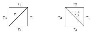
Refer to caption
Figure 11: 𝔛𝔛{\mathfrak{X}} and 𝔛+superscript𝔛{\mathfrak{X}}^{+} in the vicinity of the (-1,-1) curve.

The 1-cones of Σ𝔛subscriptΣ𝔛\Sigma_{\mathfrak{X}}, corresponding to the toric invariant divisors of 𝔛𝔛{\mathfrak{X}}, are not affected by the flop, hence can be canonically identified with those of 𝔛+superscript𝔛{\mathfrak{X}}^{+}. The 2-cones τisubscript𝜏𝑖\tau_{i} in these diagrams correspond to toric invariant 2-cycles Cisubscript𝐶𝑖C_{i}, Ci+superscriptsubscript𝐶𝑖C_{i}^{+} in the geometry. The curve classes of 𝔛𝔛{\mathfrak{X}} push forward to classes in 𝔛+superscript𝔛{\mathfrak{X}}^{+} via

ϕ([C0])=[C0+],ϕ([Ci])=[Ci+]+[C0+].formulae-sequencesubscriptitalic-ϕdelimited-[]subscript𝐶0delimited-[]superscriptsubscript𝐶0subscriptitalic-ϕdelimited-[]subscript𝐶𝑖delimited-[]superscriptsubscript𝐶𝑖delimited-[]superscriptsubscript𝐶0\displaystyle\phi_{*}([C_{0}])=-[C_{0}^{+}]\,,\quad\phi_{*}([C_{i}])=[C_{i}^{+}]+[C_{0}^{+}]\,. (6.1)

All other curve classes C𝐶\vec{C} of 𝔛𝔛{\mathfrak{X}} are mapped to their canonical counterparts in 𝔛+superscript𝔛{\mathfrak{X}}^{+}. Under appropriate analytic continuation and up to a phase factor (hence the proportional-to\propto in the following formula), the following identity then holds [39, 23, 40],

ZGW(𝔛,Q0,Q1,,Q4,Q)ZGW(𝔛+,1/Q0,Q0Q1,,Q0Q4,Q),proportional-tosubscript𝑍𝐺𝑊𝔛subscript𝑄0subscript𝑄1subscript𝑄4𝑄subscript𝑍𝐺𝑊superscript𝔛1subscript𝑄0subscript𝑄0subscript𝑄1subscript𝑄0subscript𝑄4𝑄\displaystyle Z_{GW}({\mathfrak{X}},Q_{0},Q_{1},\ldots,Q_{4},\vec{Q})\propto Z_{GW}({\mathfrak{X}}^{+},1/Q_{0},Q_{0}Q_{1},\ldots,Q_{0}Q_{4},\vec{Q})\,,

i.e.

GWg(𝔛,Q0,Q1,,Q4,Q)=GWg(𝔛+,1/Q0,Q0Q1,,Q0Q4,Q).𝐺subscript𝑊𝑔𝔛subscript𝑄0subscript𝑄1subscript𝑄4𝑄𝐺subscript𝑊𝑔superscript𝔛1subscript𝑄0subscript𝑄0subscript𝑄1subscript𝑄0subscript𝑄4𝑄\displaystyle GW_{g}({\mathfrak{X}},Q_{0},Q_{1},\ldots,Q_{4},\vec{Q})=GW_{g}({\mathfrak{X}}^{+},1/Q_{0},Q_{0}Q_{1},\ldots,Q_{0}Q_{4},\vec{Q})\,.

6.2 Proof of flop invariance via mirror symmetry

Flop invariance of Gromov-Witten invariants upon the identification (6.1) is immediate upon invoking mirror symmetry, as (6.1) maps the mirror curve of 𝔛𝔛{\mathfrak{X}} to that of 𝔛+superscript𝔛{\mathfrak{X}}^{+}. The proof is a simple computation.

Refer to caption
Figure 12: 𝔛𝔛{\mathfrak{X}} and 𝔛+superscript𝔛{\mathfrak{X}}^{+} in the vicinity of the (-1,-1) curve.

Let us introduce the notation t0,t1,t0+,t1+subscript𝑡0subscript𝑡1superscriptsubscript𝑡0superscriptsubscript𝑡1t_{0},t_{1},t_{0}^{+},t_{1}^{+} for the Kähler volume of the curve classes Ci,Ci+subscript𝐶𝑖superscriptsubscript𝐶𝑖C_{i},C_{i}^{+} corresponding to the respective 2-cones. In terms of these, we obtain for the mirror curve of 𝔛𝔛{\mathfrak{X}}

x0+x1+x2+x1x2x0eT0+x12x0eT1=0,subscript𝑥0subscript𝑥1subscript𝑥2subscript𝑥1subscript𝑥2subscript𝑥0superscript𝑒subscript𝑇0superscriptsubscript𝑥12subscript𝑥0superscript𝑒subscript𝑇10x_{0}+x_{1}+x_{2}+\frac{x_{1}x_{2}}{x_{0}}e^{T_{0}}+\frac{x_{1}^{2}}{x_{0}}e^{-T_{1}}=0\,,

while the mirror curve of 𝔛+superscript𝔛{\mathfrak{X}}^{+} is given by

x0+x1+x2+x1x2x0eT0++x1x3x2eT1+=0.subscript𝑥0subscript𝑥1subscript𝑥2subscript𝑥1subscript𝑥2subscript𝑥0superscript𝑒superscriptsubscript𝑇0subscript𝑥1subscript𝑥3subscript𝑥2superscript𝑒superscriptsubscript𝑇10x_{0}+x_{1}+x_{2}+\frac{x_{1}x_{2}}{x_{0}}e^{-T_{0}^{+}}+\frac{x_{1}x_{3}}{x_{2}}e^{-T_{1}^{+}}=0\,.

Upon invoking x3=x1x2x0eT0+subscript𝑥3subscript𝑥1subscript𝑥2subscript𝑥0superscript𝑒superscriptsubscript𝑇0x_{3}=\frac{x_{1}x_{2}}{x_{0}}e^{-T_{0}^{+}}, we easily verify that the identification (6.1) maps these curves and their associated meromorphic 1-forms λ𝜆\lambda into each other.

6.3 The BKMP conjecture

Any toric Calabi-Yau manifold 𝔛𝔛{\mathfrak{X}} with Kähler moduli Q𝑄\vec{Q} can be obtained from a sufficiently large fiducial geometry (𝔛0,Q0)subscript𝔛0subscript𝑄0({\mathfrak{X}}_{0},\vec{Q}_{0}) upon performing a series of flop transitions and taking unwanted Kähler moduli of 𝔛0subscript𝔛0{\mathfrak{X}}_{0} to \infty, see figure 13 for an example.

Refer to caption
Figure 13: Example: We obtain local 2superscript2\mathbb{P}^{2} from the fiducial geometry with 2×2222\times 2 boxes by performing five flops and then sending the Kähler parameters of the unwanted edges to \infty.

The Kähler moduli of 𝔛𝔛{\mathfrak{X}} are related to those of 𝔛0subscript𝔛0{\mathfrak{X}}_{0} by some relation Q=f(Q0)𝑄𝑓subscript𝑄0\vec{Q}=f(\vec{Q}_{0}). We have just argued that the mirror curves of 𝔛0subscript𝔛0{\mathfrak{X}}_{0} and 𝔛𝔛{\mathfrak{X}} are equal upon this identification,

𝒮𝔛,Q=𝒮𝔛0,Q0,subscript𝒮𝔛𝑄subscript𝒮subscript𝔛0subscript𝑄0{{\mathcal{S}}}_{{\mathfrak{X}},\vec{Q}}={{\mathcal{S}}}_{{\mathfrak{X}}_{0},\vec{Q_{0}}}\,,

as are the respective Gromov-Witten invariants,

GWg(𝔛,Q)=GWg(𝔛0,Q0).𝐺subscript𝑊𝑔𝔛𝑄𝐺subscript𝑊𝑔subscript𝔛0subscript𝑄0GW_{g}({\mathfrak{X}},\vec{Q})=GW_{g}({\mathfrak{X}}_{0},\vec{Q}_{0})\,.

Given the BKMP conjecture for the fiducial geometry,

GWg(𝔛0,Q0)=Fg(𝒮𝔛0,Q0),𝐺subscript𝑊𝑔subscript𝔛0subscript𝑄0subscript𝐹𝑔subscript𝒮subscript𝔛0subscript𝑄0GW_{g}({\mathfrak{X}}_{0},\vec{Q}_{0})=F_{g}({{\mathcal{S}}}_{{\mathfrak{X}}_{0},\vec{Q}_{0}})\,,

its validity thus follows for any toric Calabi-Yau manifold:

   GWg(𝔛,Q)=Fg(𝒮𝔛,Q)𝐺subscript𝑊𝑔𝔛𝑄subscript𝐹𝑔subscript𝒮𝔛𝑄\displaystyle GW_{g}({\mathfrak{X}},\vec{Q})=F_{g}({{\mathcal{S}}}_{{\mathfrak{X}},\vec{Q}})   

7 Conclusion

Taking our matrix model from [1] as a starting point and imposing certain minimality conditions on the spectral curve, we have thus derived the BKMP conjecture, for closed topological strings, for all toric Calabi-Yau manifolds in the large radius limit. As we have emphasized throughout, elevating our procedure to a formal proof of the conjecture requires a more rigorous derivation of the spectral curve of our matrix model.

It should also be possible to extend our argument to open Gromov-Witten invariants by invoking loop operators, which relate closed to open invariants. In [3], such an operator was defined in the matrix model context. An analogous operator should also exist in the theory of Gromov-Witten invariants [41]. Establishing the equivalence of these two loop operators would allow us to conclude that the Wn(g)superscriptsubscript𝑊𝑛𝑔W_{n}^{(g)}’s of the spectral curve 𝒮𝔛subscript𝒮𝔛{{\mathcal{S}}}_{{\mathfrak{X}}} are the open Gromov-Witten invariants of 𝔛𝔛{\mathfrak{X}}.

Finally, our treatment of the BKMP conjecture took place at large radius. One should study the behavior of the matrix model as one moves away from large radius e.g. to orbifold points, and see whether the phase transitions of the topological string are captured accurately by the matrix model. Of course, the main tool on the topological string side employed in this work, the topological vertex, is no longer applicable in these regions of moduli space.

Acknowledgments

B.E. and O.M. would like to thank M. Bertola, J. Harnad, V. Bouchard, M. Mariño, M. Mulase, H.  Ooguri, N. Orantin, B. Safnuk, for useful and fruitful discussions on this subject. A.K. would like to thank Vincent Bouchard and Ilarion Melnikov for helpful conversations. The work of B.E. is partly supported by the Enigma European network MRT-CT-2004-5652, ANR project GranMa ”Grandes Matrices Aléatoires” ANR-08-BLAN-0311-01, by the European Science Foundation through the Misgam program, by the Quebec government with the FQRNT. B.E. would like to thank the AIM, as well as the organizers and all participants to the workshop [42] held at the AIM june 2009. O.M. would like to thank the CRM (Centre de recheche mathématiques de Montréal, QC, Canada) for its hospitality.

Appendix A The matrix model

In this appendix, which is mainly a reprint of section 4 of [1], we present the matrix model which reproduces the topological string partition function on the fiducial geometry 𝔛0subscript𝔛0{\mathfrak{X}}_{0}, and whose spectral curve we derive in the text.

SConsider the fiducial geometry 𝔛0subscript𝔛0{\mathfrak{X}}_{0} of size (n+1)×(m+1)𝑛1𝑚1(n+1)\times(m+1), with Kähler parameters ti,j=ai,jai,j+1subscript𝑡𝑖𝑗subscript𝑎𝑖𝑗subscript𝑎𝑖𝑗1t_{i,j}=a_{i,j}-a_{i,j+1}, ri,j=ai,j+1ai+1,jsubscript𝑟𝑖𝑗subscript𝑎𝑖𝑗1subscript𝑎𝑖1𝑗r_{i,j}=a_{i,j+1}-a_{i+1,j}, and si,jsubscript𝑠𝑖𝑗s_{i,j}, as depicted in figure 1. We write

ai=(a0,i,a1,i,,an,i).subscript𝑎𝑖subscript𝑎0𝑖subscript𝑎1𝑖subscript𝑎𝑛𝑖\vec{a}_{i}=(a_{0,i},a_{1,i},\dots,a_{n,i}).

Assume that the external representations are fixed to αm+1=(α0,m+1,α1,m+1,,αn,m+1)subscript𝛼𝑚1subscript𝛼0𝑚1subscript𝛼1𝑚1subscript𝛼𝑛𝑚1\vec{\alpha}_{m+1}=(\alpha_{0,m+1},\alpha_{1,m+1},\dots,\alpha_{n,m+1}) on the upper line, and α0=(α0,0,α1,0,,αn,0)subscript𝛼0subscript𝛼00subscript𝛼10subscript𝛼𝑛0\vec{\alpha}_{0}=(\alpha_{0,0},\alpha_{1,0},\dots,\alpha_{n,0}) on the lower line. For the most part, we will choose these to be trivial.


We now define the following matrix integral 𝒵MMsubscript𝒵MM{\cal Z}_{\rm MM} (MM for Matrix Model),

𝒵MM(Q,gs,αm+1,α0T)subscript𝒵MM𝑄subscript𝑔𝑠subscript𝛼𝑚1superscriptsubscript𝛼0𝑇\displaystyle{\cal Z}_{\rm MM}(Q,g_{s},\vec{\alpha}_{m+1},\vec{\alpha}_{0}^{T}) =\displaystyle= Δ(X(αm+1))Δ(X(α0))i=0m+1HN(Γi)𝑑Mii=1m+1HN(+)𝑑RiΔ𝑋subscript𝛼𝑚1Δ𝑋subscript𝛼0superscriptsubscriptproduct𝑖0𝑚1subscriptsubscript𝐻𝑁subscriptΓ𝑖differential-dsubscript𝑀𝑖superscriptsubscriptproduct𝑖1𝑚1subscriptsubscript𝐻𝑁subscriptdifferential-dsubscript𝑅𝑖\displaystyle\Delta(X(\vec{\alpha}_{m+1}))\,\,\Delta(X(\vec{\alpha}_{0}))\,\,\prod_{i=0}^{m+1}\int_{H_{N}(\Gamma_{i})}dM_{i}\,\prod_{i=1}^{m+1}\int_{H_{N}({\mathbb{R}}_{+})}\,dR_{i} (A.1)
i=1me1gstr[Vai(Mi)Vai1(Mi)]i=1me1gstr[Vai1(Mi1)Vai(Mi1)]superscriptsubscriptproduct𝑖1𝑚superscript𝑒1subscript𝑔𝑠trdelimited-[]subscript𝑉subscript𝑎𝑖subscript𝑀𝑖subscript𝑉subscript𝑎𝑖1subscript𝑀𝑖superscriptsubscriptproduct𝑖1𝑚superscript𝑒1subscript𝑔𝑠trdelimited-[]subscript𝑉subscript𝑎𝑖1subscript𝑀𝑖1subscript𝑉subscript𝑎𝑖subscript𝑀𝑖1\displaystyle\prod_{i=1}^{m}e^{{-1\over g_{s}}\,{\rm tr\,}\left[V_{\vec{a}_{i}}(M_{i})-V_{\vec{a}_{i-1}}(M_{i})\right]}\,\,\,\prod_{i=1}^{m}e^{{-1\over g_{s}}\,{\rm tr\,}\left[V_{\vec{a}_{i-1}}(M_{i-1})-V_{\vec{a}_{i}}(M_{i-1})\right]}
i=1m+1e1gstr(MiMi1)Rii=1me(Si+iπgs)trlnMisuperscriptsubscriptproduct𝑖1𝑚1superscript𝑒1subscript𝑔𝑠trsubscript𝑀𝑖subscript𝑀𝑖1subscript𝑅𝑖superscriptsubscriptproduct𝑖1𝑚superscript𝑒subscript𝑆𝑖𝑖𝜋subscript𝑔𝑠trsubscript𝑀𝑖\displaystyle\prod_{i=1}^{m+1}e^{{1\over g_{s}}{\rm tr\,}(M_{i}-M_{i-1})R_{i}}\,\,\,\prod_{i=1}^{m}e^{(S_{i}+{i\pi\over g_{s}})\,{\rm tr\,}\,\ln M_{i}}\,
etrlnf0(M0)etrlnfm+1(Mm+1)i=1metrlnfi(Mi).superscript𝑒trsubscript𝑓0subscript𝑀0superscript𝑒trsubscript𝑓𝑚1subscript𝑀𝑚1superscriptsubscriptproduct𝑖1𝑚superscript𝑒trsubscript𝑓𝑖subscript𝑀𝑖\displaystyle e^{{\rm tr\,}\ln f_{0}(M_{0})}\,\,e^{{\rm tr\,}\ln f_{m+1}(M_{m+1})}\,\,\prod_{i=1}^{m}e^{{\rm tr\,}\ln f_{i}(M_{i})}\,.

All matrices are taken of size

N=(n+1)d.𝑁𝑛1𝑑N=(n+1)\,d\,.

d𝑑d denotes a cut-off on the size of the matrices, on which, as discussed in section 5.2.1, the partition function depends only non-perturbatively. We have introduced the notation

X(αm+1)=diag(X(αm+1)i)i=1,,N,X(αm+1)jd+k=qhk(αj,m+1),formulae-sequence𝑋subscript𝛼𝑚1diagsubscript𝑋subscriptsubscript𝛼𝑚1𝑖𝑖1𝑁𝑋subscriptsubscript𝛼𝑚1𝑗𝑑𝑘superscript𝑞subscript𝑘subscript𝛼𝑗𝑚1X(\vec{\alpha}_{m+1})={\rm diag}(X(\vec{\alpha}_{m+1})_{i})_{i=1,\dots,N}\,\,,\qquad X(\vec{\alpha}_{m+1})_{jd+k}=q^{h_{k}(\alpha_{j,m+1})},
X(α0)=diag(X(α0)i)i=1,,N,X(α0)jd+k=qhk(αj,0),formulae-sequence𝑋subscript𝛼0diagsubscript𝑋subscriptsubscript𝛼0𝑖𝑖1𝑁𝑋subscriptsubscript𝛼0𝑗𝑑𝑘superscript𝑞subscript𝑘subscript𝛼𝑗0X(\vec{\alpha}_{0})={\rm diag}(X(\vec{\alpha}_{0})_{i})_{i=1,\dots,N}\,\,,\qquad X(\vec{\alpha}_{0})_{jd+k}=q^{h_{k}(\alpha_{j,0})},

for k=1,,d𝑘1𝑑k=1,\ldots,d, j=0,,n𝑗0𝑛j=0,\ldots,n, where

hi(γ)=γii+d+a.subscript𝑖𝛾subscript𝛾𝑖𝑖𝑑𝑎h_{i}(\gamma)=\gamma_{i}-i+d+a\,. (A.2)

Δ(X)=i<j(XiXj)Δ𝑋subscriptproduct𝑖𝑗subscript𝑋𝑖subscript𝑋𝑗\Delta(X)=\prod_{i<j}(X_{i}-X_{j}) is the Vandermonde determinant. The potentials Vai(x)subscript𝑉subscript𝑎𝑖𝑥V_{\vec{a}_{i}}(x) are given by

Va(X)=gsj=0nln(g(qaj/X))subscript𝑉𝑎𝑋subscript𝑔𝑠superscriptsubscript𝑗0𝑛𝑔superscript𝑞subscript𝑎𝑗𝑋V_{\vec{a}}(X)=-g_{s}\,\sum_{j=0}^{n}\ln{\left(g(q^{a_{j}}/X)\right)} (A.3)

in terms of the q𝑞q-product

g(x)=n=1(11xqn).𝑔𝑥superscriptsubscriptproduct𝑛111𝑥superscript𝑞𝑛\displaystyle g(x)=\prod_{n=1}^{\infty}(1-{1\over x}\,q^{n})\,.

For i=1,,m𝑖1𝑚i=1,\dots,m, we have defined

fi(x)=j=0ng(1)2e(12+iπlnq)ln(xq1aj,i)e(ln(xq1aj,i))22gsg(xq1aj,i)g(qaj,i/x).subscript𝑓𝑖𝑥superscriptsubscriptproduct𝑗0𝑛𝑔superscript12superscript𝑒12𝑖𝜋𝑞𝑥superscript𝑞1subscript𝑎𝑗𝑖superscript𝑒superscript𝑥superscript𝑞1subscript𝑎𝑗𝑖22subscript𝑔𝑠𝑔𝑥superscript𝑞1subscript𝑎𝑗𝑖𝑔superscript𝑞subscript𝑎𝑗𝑖𝑥f_{i}(x)=\prod_{j=0}^{n}{g(1)^{2}\,\,e^{({1\over 2}+{i\pi\over\ln q})\,\ln{(xq^{1-a_{j,i}})}}\,\,e^{{(\ln{(xq^{1-a_{j,i}})})^{2}\over 2g_{s}}}\over g(x\,q^{1-a_{j,i}})\,g(q^{a_{j,i}}/x)\,}\,.

The denominator of these functions induces simple poles at x=qaj,i+l𝑥superscript𝑞subscript𝑎𝑗𝑖𝑙x=q^{a_{j,i}+l} for j=0,,n𝑗0𝑛j=0,\dots,n and l𝑙l\in\mathbb{Z}. The numerator is chosen such that they satisfy the relation fi(qx)=fi(x)subscript𝑓𝑖𝑞𝑥subscript𝑓𝑖𝑥f_{i}(qx)=f_{i}(x). This enforces a simple l𝑙l-dependence of the residues taken at x=qaj,i+l𝑥superscript𝑞subscript𝑎𝑗𝑖𝑙x=q^{a_{j,i}+l}, given by a prefactor qlsuperscript𝑞𝑙q^{l} – a fact which will be important in the following. These residues are in fact given by

Resqaj,i+lfi(x)=qaj,i+lf^j,i=qaj,i+lkjg(1)2e(12+iπlnq)(1+aj,iak,i)lnqe(ln(q1+aj,iak,i))22gsg(qaj,iak,i)(1qak,iaj,i)g(qak,iaj,i),subscriptRessuperscript𝑞subscript𝑎𝑗𝑖𝑙subscript𝑓𝑖𝑥superscript𝑞subscript𝑎𝑗𝑖𝑙subscript^𝑓𝑗𝑖superscript𝑞subscript𝑎𝑗𝑖𝑙subscriptproduct𝑘𝑗𝑔superscript12superscript𝑒12𝑖𝜋𝑞1subscript𝑎𝑗𝑖subscript𝑎𝑘𝑖𝑞superscript𝑒superscriptsuperscript𝑞1subscript𝑎𝑗𝑖subscript𝑎𝑘𝑖22subscript𝑔𝑠𝑔superscript𝑞subscript𝑎𝑗𝑖subscript𝑎𝑘𝑖1superscript𝑞subscript𝑎𝑘𝑖subscript𝑎𝑗𝑖𝑔superscript𝑞subscript𝑎𝑘𝑖subscript𝑎𝑗𝑖\mathop{{\rm Res}\,}_{q^{a_{j,i}+l}}f_{i}(x)=q^{a_{j,i}+l}\,\,\hat{f}_{j,i}=-\,q^{a_{j,i}+l}\,\,\prod_{k\neq j}{g(1)^{2}\,\,e^{({1\over 2}+{i\pi\over\ln q})\,(1+a_{j,i}-a_{k,i})\ln q}\,\,e^{{(\ln{(q^{1+a_{j,i}-a_{k,i}})})^{2}\over 2g_{s}}}\over g(q^{a_{j,i}-a_{k,i}})\,(1-q^{a_{k,i}-a_{j,i}})g(q^{a_{k,i}-a_{j,i}})}\,, (A.4)

where f^j,isubscript^𝑓𝑗𝑖\hat{f}_{j,i} is independent of the integer l𝑙l.

The parameters Sisubscript𝑆𝑖S_{i} are defined by

Si=s0,i1+t0,i1=sj,i1k<jtk,i+kjtk,i1.subscript𝑆𝑖subscript𝑠0𝑖1subscript𝑡0𝑖1subscript𝑠𝑗𝑖1subscript𝑘𝑗subscript𝑡𝑘𝑖subscript𝑘𝑗subscript𝑡𝑘𝑖1S_{i}=s_{0,i-1}+t_{0,i-1}=s_{j,i-1}-\sum_{k<j}t_{k,i}+\sum_{k\leq j}t_{k,i-1}\,. (A.5)

The final equality holds for arbitrary j𝑗j [1].

For i=0𝑖0i=0 and i=m+1𝑖𝑚1i=m+1, we define

f0(x)=1j=0ni=1d(xqhi(αj,0)),subscript𝑓0𝑥1superscriptsubscriptproduct𝑗0𝑛superscriptsubscriptproduct𝑖1𝑑𝑥superscript𝑞subscript𝑖subscript𝛼𝑗0f_{0}(x)={1\over\prod_{j=0}^{n}\prod_{i=1}^{d}(x-q^{h_{i}(\alpha_{j,0})})}\,,
fm+1(x)=1j=0ni=1d(xqhi(αj,m+1)).subscript𝑓𝑚1𝑥1superscriptsubscriptproduct𝑗0𝑛superscriptsubscriptproduct𝑖1𝑑𝑥superscript𝑞subscript𝑖subscript𝛼𝑗𝑚1f_{m+1}(x)={1\over\prod_{j=0}^{n}\prod_{i=1}^{d}(x-q^{h_{i}(\alpha_{j,m+1})})}\,.

Notice that if the representations α0subscript𝛼0\vec{\alpha}_{0} or αm+1subscript𝛼𝑚1\vec{\alpha}_{m+1} are trivial, i.e. hi(αj,0)=di+aj,0subscript𝑖subscript𝛼𝑗0𝑑𝑖subscript𝑎𝑗0h_{i}(\alpha_{j,0})=d-i+a_{j,0} or hi(αj,m+1)=di+aj,m+1subscript𝑖subscript𝛼𝑗𝑚1𝑑𝑖subscript𝑎𝑗𝑚1h_{i}(\alpha_{j,m+1})=d-i+a_{j,m+1}, we have

f0(x)=j=0ng(xq1aj,0d)xdg(xq1aj,0),fm+1(x)=j=0ng(xq1aj,m+1d)xdg(xq1aj,m+1)formulae-sequencesubscript𝑓0𝑥superscriptsubscriptproduct𝑗0𝑛𝑔𝑥superscript𝑞1subscript𝑎𝑗0𝑑superscript𝑥𝑑𝑔𝑥superscript𝑞1subscript𝑎𝑗0subscript𝑓𝑚1𝑥superscriptsubscriptproduct𝑗0𝑛𝑔𝑥superscript𝑞1subscript𝑎𝑗𝑚1𝑑superscript𝑥𝑑𝑔𝑥superscript𝑞1subscript𝑎𝑗𝑚1f_{0}(x)=\prod_{j=0}^{n}{g(x\,q^{1-a_{j,0}-d})\over x^{d}\,g(x\,q^{1-a_{j,0}})}\,,\hskip 28.45274ptf_{m+1}(x)=\prod_{j=0}^{n}{g(x\,q^{1-a_{j,m+1}-d})\over x^{d}\,g(x\,q^{1-a_{j,m+1}})}

respectively. The functions f0subscript𝑓0f_{0} and fm+1subscript𝑓𝑚1f_{m+1} have simple poles at x=qhl(αj,0)𝑥superscript𝑞subscript𝑙subscript𝛼𝑗0x=q^{h_{l}(\alpha_{j,0})} (resp. x=qhl(αj,m+1)𝑥superscript𝑞subscript𝑙subscript𝛼𝑗𝑚1x=q^{h_{l}(\alpha_{j,m+1})}) for l=1,,d𝑙1𝑑l=1,\dots,d, with residue

f^j,0;l=Resqhl(αj,0)f0(x)=1jji=1d(qhl(αj,0)qhi(αj,0))1il(qhl(αj,0)qhi(αj,0)),subscript^𝑓𝑗0𝑙subscriptRessuperscript𝑞subscript𝑙subscript𝛼𝑗0subscript𝑓0𝑥1subscriptproductsuperscript𝑗𝑗superscriptsubscriptproduct𝑖1𝑑superscript𝑞subscript𝑙subscript𝛼𝑗0superscript𝑞subscript𝑖subscript𝛼superscript𝑗01subscriptproduct𝑖𝑙superscript𝑞subscript𝑙subscript𝛼𝑗0superscript𝑞subscript𝑖subscript𝛼𝑗0\hat{f}_{j,0;l}=\mathop{{\rm Res}\,}_{q^{h_{l}(\alpha_{j,0})}}f_{0}(x)={1\over\prod_{j^{\prime}\neq j}\prod_{i=1}^{d}(q^{h_{l}(\alpha_{j,0})}-q^{h_{i}(\alpha_{j^{\prime},0})})}\,{1\over\prod_{i\neq l}(q^{h_{l}(\alpha_{j,0})}-q^{h_{i}(\alpha_{j,0})})}\,,
f^j,m+1;l=Resqhl(αj,m+1)fm+1(x)=1jji=1d(qhl(αj,m+1)qhi(αj,m+1))1il(qhl(αj,m+1)qhi(αj,m+1)).subscript^𝑓𝑗𝑚1𝑙subscriptRessuperscript𝑞subscript𝑙subscript𝛼𝑗𝑚1subscript𝑓𝑚1𝑥1subscriptproductsuperscript𝑗𝑗superscriptsubscriptproduct𝑖1𝑑superscript𝑞subscript𝑙subscript𝛼𝑗𝑚1superscript𝑞subscript𝑖subscript𝛼superscript𝑗𝑚11subscriptproduct𝑖𝑙superscript𝑞subscript𝑙subscript𝛼𝑗𝑚1superscript𝑞subscript𝑖subscript𝛼𝑗𝑚1\hat{f}_{j,m+1;l}=\mathop{{\rm Res}\,}_{q^{h_{l}(\alpha_{j,m+1})}}f_{m+1}(x)={1\over\prod_{j^{\prime}\neq j}\prod_{i=1}^{d}(q^{h_{l}(\alpha_{j,m+1})}-q^{h_{i}(\alpha_{j^{\prime},m+1})})}\,{1\over\prod_{i\neq l}(q^{h_{l}(\alpha_{j,m+1})}-q^{h_{i}(\alpha_{j,m+1})})}\,.

The l𝑙l dependence here is more intricate than above, but this will not play any role since the partitions αj,0subscript𝛼𝑗0\alpha_{j,0} and αj,m+1subscript𝛼𝑗𝑚1\alpha_{j,m+1} are kept fixed, and not summed upon.


The integration domains for the matrices Risubscript𝑅𝑖R_{i} are HN(+N)subscript𝐻𝑁superscriptsubscript𝑁H_{N}(\mathbb{R}_{+}^{N}), i.e. the set of hermitian matrices having only positive eigenvalues. For the matrices Mi,i=1,,mformulae-sequencesubscript𝑀𝑖𝑖1𝑚M_{i},i=1,\dots,m, the integration domains are HN(Γi)subscript𝐻𝑁subscriptΓ𝑖H_{N}(\Gamma_{i}), where

Γi=j=0n(γj,i)d.subscriptΓ𝑖superscriptsubscriptproduct𝑗0𝑛superscriptsubscript𝛾𝑗𝑖𝑑\Gamma_{i}=\prod_{j=0}^{n}\,(\gamma_{j,i})^{d}\,.

γj,isubscript𝛾𝑗𝑖\gamma_{j,i} is defined as a contour which encloses all points of the form qaj,i+superscript𝑞subscript𝑎𝑗𝑖q^{a_{j,i}+\mathbb{N}}, and does not intersect any contours γk,lsubscript𝛾𝑘𝑙\gamma_{k,l}, (j,i)(k,l)𝑗𝑖𝑘𝑙(j,i)\neq(k,l). For this to be possible, we must require that the differences aj,iaj,isubscript𝑎𝑗𝑖subscript𝑎superscript𝑗superscript𝑖a_{j,i}-a_{j^{\prime},i^{\prime}} be non-integer. The normalized logarithms of two such contours are depicted in figure 14.

Refer to caption
Figure 14: Two contours surrounding points a+𝑎a+\mathbb{N} and b+𝑏b+\mathbb{N}, such that ab𝑎𝑏a-b\notin\mathbb{Z}.

We have defined

HN(Γi)={M=UΛU,UU(N),Λ=diag(λ1,,λN)Γi},subscript𝐻𝑁subscriptΓ𝑖formulae-sequence𝑀𝑈Λsuperscript𝑈formulae-sequence𝑈𝑈𝑁Λdiagsubscript𝜆1subscript𝜆𝑁subscriptΓ𝑖H_{N}(\Gamma_{i})=\{M=U\,\Lambda\,U^{\dagger}\,,\quad U\in U(N)\,,\,\,\,\Lambda={\rm diag}(\lambda_{1},\dots,\lambda_{N})\,\in\Gamma_{i}\}\,,

i.e. HN(Γi)subscript𝐻𝑁subscriptΓ𝑖H_{N}(\Gamma_{i}) is the set of normal matrices with eigenvalues on ΓisubscriptΓ𝑖\Gamma_{i}. By definition, the measure on HN(Γi)subscript𝐻𝑁subscriptΓ𝑖H_{N}(\Gamma_{i}) is (see [24])

dM=1N!Δ(Λ)2dUdΛ,𝑑𝑀1𝑁ΔsuperscriptΛ2𝑑𝑈𝑑ΛdM={1\over N!}\,\,\Delta(\Lambda)^{2}\,\,dU\,d\Lambda\,, (A.6)

where dU𝑑𝑈dU is the Haar measure on U(N)𝑈𝑁U(N), and dΛ𝑑Λd\Lambda is the product of the measures for each eigenvalue along its integration path.

The integration domains for the matrices M0subscript𝑀0M_{0}, Mm+1subscript𝑀𝑚1M_{m+1} are HN(Γ0)subscript𝐻𝑁subscriptΓ0H_{N}(\Gamma_{0}), HN(Γm+1)subscript𝐻𝑁subscriptΓ𝑚1H_{N}(\Gamma_{m+1}) respectively, where

Γ0=(j=0nγj,0)N,Γm+1=(j=0nγj,m+1)N.formulae-sequencesubscriptΓ0superscriptsuperscriptsubscript𝑗0𝑛subscript𝛾𝑗0𝑁subscriptΓ𝑚1superscriptsuperscriptsubscript𝑗0𝑛subscript𝛾𝑗𝑚1𝑁\Gamma_{0}=(\sum_{j=0}^{n}\gamma_{j,0})^{N}\,,\qquad\quad\Gamma_{m+1}=(\sum_{j=0}^{n}\gamma_{j,m+1})^{N}\,. (A.7)

References