MILCA, a Modified Internal Linear Combination Algorithm to extract astrophysical emissions from multi-frequency sky maps.
The analysis of current Cosmic Microwave Background (CMB) experiments is based on the interpretation of multi-frequency sky maps in terms of different astrophysical components and it requires specifically tailored component separation algorithms. In this context, Internal Linear Combination (ILC) methods have been extensively used to extract the CMB emission from the WMAP multi-frequency data. We present here a Modified Internal Linear Component Algorithm (MILCA) that generalizes the ILC approach to the case of multiple astrophysical components for which the electromagnetic spectrum is known. In addition MILCA corrects for the intrinsic noise bias in the standard ILC approach and extends it to an hybrid space-frequency representation of the data. It also allows us to use external templates to minimize the contribution of extra components but still using only a linear combination of the input data. We apply MILCA to simulations of the Planck satellite data at the HFI frequency bands. We explore the possibility of reconstructing the Galactic molecular CO emission on the Planck maps as well as the thermal Sunyaev-Zeldovich effect. We conclude that MILCA is able to accurately estimate those emissions and it has been successfully used for this purpose within the Planck collaboration.
Key Words.:
Cosmic Background Radiation - Methods: data analysis1 Introduction
Multi-frequency Comic Microwave Background (CMB) experiments such as WMAP Bennett et al. (2003) and Planck The Planck Collaboration (2006) spacecraft missions, observes a mixture of astrophysical emissions. Most of them follow different emission laws (e.g. CMB anisotropies, thermal Sunyaev-Zel’dovich (tSZ) effect Sunyaev & Zeldovich (1972), thermal dust, Cosmic Infrared Background (CIB), synchrotron, molecular cloud emission, etc.).
It is thus possible to separate the mixed astrophysical sources taking advantage of the specific emission laws of each astrophysical component.
The separation of astrophysical sources from a set of multi-channel observations of the millimeter and sub-millimeter sky is an important step in the scientific exploitation of such data. In this context, a large number of methods have been developed.
These component separation techniques can be separated in various categories depending on the degree and nature of the prior information used.
For example, Maximum Likelihood techniques (e.g., Commander, Eriksen et al., 2008) and Maximum of Entropy methods (e.g. (Hobson et al., 1998; Stolyarov et al., 2002))
assume that the electromagnetic spectrum of the different components is known or that it can be easily parametrized. By contrast,
blind (or semi-blind) component separation methods such as, Spectral Matching ICA (Cardoso et al., 2008; Delabrouille et al., 2003),
PolEMICA (Aumont & Macías-Pérez, 2007), FastICA (Maino et al., 2002), CCA (Bonaldi et al., 2006) or GMCA (Bobin et al., 2008) exploit the spectral
and spatial diversity of the components and need no a priori on those. In a different way, ILC (Internal Linear Combination) techniques
(Bennett et al., 2003; Eriksen et al., 2004; Remazeilles et al., 2011) aim at preserving an astrophysical component for which the electromagnetic
spectrum is known, by minimizing the variance in the reconstructed signal.
Standard ILC methods are very popular because of their simplicity and robustness.
However, as discussed by Vio & Andreani (2008), they are biased by the noise contribution to the variance of the final map.
This bias reduces the efficiency of the algorithm in poor signal to noise conditions.
Furthermore, they do not fully exploit
the spatial and spectral diversity to minimize the contribution from other sky components
for which the electromagnetic spectrum is poorly, or not at all, known.
The ILC methods also assume that the component of interest is statistically independent from the other ones.
If the statistical independence assumption can be made for the CMB, it is not the case for all the astrophysical components of the millimeter and sub-millimeter sky. Indeed, for example galactic foregrounds such as thermal dust, synchrotron and molecular cloud emission are highly correlated over the sky. Such correlations can also be observed for extra-galactic components like tSZ and extra-galactic point sources.
We present, in this article the Modified Internal Linear Combination Algorithm (MILCA) that generalizes standard ILC techniques
to multiple constraints, in order to reduce the level of contamination by other astrophysical emissions.
We will show that MILCA also corrects for the noise bias of the standard ILC solution and blindly minimizes the contribution from unknown or poorly constrained sky components.
The paper is organized as follows.
In section 2 we present our modeling the millimeter and sub-milimeter sky. Then, in Sect. 3 we address the problem of generalizing the ILC algorithm to multiple constraints. Section 4 discusses possible bias in the ILC algorithm. In Sect. 5 we propose modifications to the standard ILC estimator in order to minimize the
instrumental noise and contamination from other astrophysical components. Finally we apply MILCA on Planck simulated datasets, focusing on the extraction of the tSZ effect(Sect. 6) and molecular cloud emission (Sect. 7).
2 Simulation of the microwave sky seen by Planck
2.1 The Planck mission and the sub-millimeter sky
The Planck mission (Planck Collaboration I, 2011, 2013) is the third space mission,
after the COBE (Smoot et al., 1992; Bennett et al., 1996) and the WMAP (Hinshaw et al., 2003, 2009; Bennett et al., 2003) missions,
devoted to the study of the microwave and sub-mm emissions, and especially to the Cosmic Microwave Background radiation (CMB).
Planck, as other CMB experiments, observes the sky emission in different frequency bands.
In particular, Planck has two instruments: the Low Frequency Instrument (LFI) (Bersanelli et al., 2010; Mennella et al., 2011) which has three frequency bands
centered at 30, 44 and 70 GHz, and the High Frequency Instrument (HFI) (Lamarre et al., 2010; Planck HFI Core Team, 2011) which has six frequency bands
centered at 100, 143, 217, 353, 545 and 857 GHz.
The large number of detectors and their high sensitivity, make the Planck mission the first CMB experiment expected to be limited
by our knowledge of the foreground emissions rather than by instrumental noise.
At the Planck frequencies the main astrophysical emissions are: the diffuse Galactic free-free, synchrotron, and thermal dust (The Planck Collaboration, 2006) emissions; the
anomalous microwave emission (AME, Planck Collaboration XX, 2011) ; the molecular Galactic emissions (mainly 12CO in the 100, 217 and 353 GHz bands, Planck Collaboration XIII, 2013b),
the emission from Galactic and extra galactic point sources (radio and infrared sources, Planck Collaboration Int. VII, 2013; Planck Collaboration VII, 2011; Planck Collaboration XVIII, 2011); and the thermal
Sunyaev-Zeldovich effect (Sunyaev & Zeldovich, 1972) in clusters of galaxies (Planck Collaboration VIII, 2011; Planck Collaboration XXIX, 2013).
2.2 Simulations of the sub-millimeter sky
We have simulated the microwave and sub-millimeter sky observed by Planck using a set of template maps to reproduce astrophysical components.
Within those components we include CMB, diffuse Galactic emissions (synchrotron, free-free and thermal dust), Galactic CO emission, Galactic and extra-galactic point sources,
CIB and tSZ emissions. We did not include in the simulation the Anomalous Microwave Emission (AME) for which a template is not available and
that we expect to be subdominant for the following analyses.
The CMB was simulated using a random gaussian field as defined by the Planck best-fit CMB angular power spectrum (Planck Collaboration XV, 2013; Planck Collaboration XVI, 2013).
The thermal dust emission was modeled using the reprocessed IRAS maps at 100 m (IRIS Miville-Deschênes & Lagache, 2005) extrapolated to the Planck frequencies assuming a grey body emission law (e.g. Desert et al., 1990). with constant temperature, K) and spectral index .
The synchrotron emission was simulated using the 408 MHz full-sky map from Haslam et al. (1981) corrected for free-free emission assuming an emission law with a spatially constant spectral index of in antenna-temperature units (Davies et al., 1996).
The Galactic free-free emission was modeled using the full-sky map (Finkbeiner, 2003) and an electron temperature of K as proposed by Dickinson et al. (2003) and a spatially constant spectral index of in antenna-temperature units.
The CO emission was modeled using the J=1-0 CO map from Dame et al. (2001), the transmission in Planck’s sky maps have been computed assuming a fluctuation of 10% in the bandpass amplitude (Planck Collaboration XIII, 2013a). Finally, we add gaussian white noise in the map with the expected levels for the Planck mission (Planck Collaboration I, 2013).
We also add radio point sources using the sources in the NVSS catalog and extrapolating their flux to the Planck frequencies assuming a random spectral index for each source
derived from a Gaussian distribution with a mean of and a standard deviation of in antenna temperature units (Planck Collaboration XIII, 2011).
Extra-galactic infra-red (IR) astrophysical emissions can be decomposed into two categories, a poissonian contribution, composed by point sources, and a diffuse contribution, the clustered CIB. To model IR point sources we also used a randomly distributed sources with random spectral index for each source (with a mean of and a standard deviation of in antenna temperature units (Planck Collaboration XIII, 2011)). For the CIB emission, we assumed a random gaussian distribution following the CIB power spectra as measured by Planck (Planck Collaboration XVIII, 2011) and constant correlation factors across frequencies.
The tSZ emission is produced by the hot and dense gas of electrons, such gas can be found in galaxy clusters or in the WHIM. In this study we only account for the emission from X-ray known galaxy clusters. To do so, the tSZ was simulated using a universal electron pressure profile from Arnaud et al. (2010) and
physical parameters for clusters from the MCXC catalog (Piffaretti et al., 2011).
3 Generalising ILC method
The total emission observed at a given frequency channel map, , can be expressed as the superposition of astrophysical components and instrumental noise
| (1) |
where denotes the pixel number. are the maps of the astrophysical components (CMB and foregrounds) in the data and is the instrumental noise. is the mixing matrix given by
| (2) |
with the spectral dependence of the -th component and the spectral response of the -th channel.
Assuming that the mixing matrix is constant across the sky, equation 1 can be written in a more compact manner as
| (3) |
where and are vectors containing the total and noise maps for the observation channels, is a matrix corresponding to the maps of the astrophysical components. is the mixing matrix with dimensions .
3.1 Internal Linear Combination algorithm
The Internal Linear Combination algorithm (Bennett et al., 2003) assumes that the astrophysical component to be reconstructed, , can be obtained as a linear combination of the input observational maps
| (4) |
The weights, , of the linear combination are computed by minimizing the variance of the output map,
| (5) |
under constraints on the emission spectrum of . is the covariance
matrix of the observed maps, , averaged across pixels.
For the CMB and assuming that the maps are given in thermodynamic temperature units, the constraint simply read (Bennett et al., 2003; Eriksen et al., 2004)
| (6) |
More generally, for an astrophysical component with emission spectrum, , the constraints can be written as
| (7) |
Notice that is related to the mixing matrix, , by , where is an dimension vector for which all elements are set to zero except the -th element that is set to 1.
Linear system solution
Weights can be computed solving a linear system using Lagrange multipliers
| (8) |
where is a Lagrange multiplier. The final linear system can be expressed in the form
| (15) |
3.2 Multiple spectral constraints
In some particular cases, the emission spectra of various astrophysical components may be known with sufficient accuracy. Thus, it is possible to use multiple constraints (i.e., ) for the minimization process to extract some of the astrophysical components and to reject some of the others. In practice, we can write those constraints as
| (19) |
where are the number of rejected components.
Remazeilles et al. (2011) has shown that 2 components can be constrained and simultaneously recovered. We propose here a generalization of this method to an arbitrarily large number of constraints. Defining as a matrix with elements such that
equation 15 can be generalized to
| (26) |
where are the Lagrange multipliers and . The solution of the system can then be written as
| (27) |
with the dimension matrix containing the weights extracting each constrained components. The first line of this matrix contains the weights for the extraction of the components of interest, .
Notice that in the relation , is now a matrix.
4 Bias in the standard ILC estimator
The ILC estimator as presented above is biased. This bias can have several origins:
-
•
correlation between the wanted components and the other astrophysical components
-
•
differences between the true emission laws and the constraints used to minimize the variance. These differences can be produced by calibration uncertainties Dick et al. (2010) or by discrepancies between the used emission laws and the effective ones.
-
•
noise-induced correlations
4.1 Intrinsic bias
We first characterize the bias in the ILC estimator proposed in Eq. (16), neglecting the contribution of the instrumental noise. In this situation, we can write the channel covariance matrix as:
| (28) |
with the dimension covariance matrix of the astrophysical components. The matrix has a dimension but has a rank: , by construction; as for , it has a rank . From here, three cases are possible for the matrix inversion:
-
•
(1) : There are more physical components than channels. It is not possible to describe with an dimension sub-space. The dimension subspace which describe the matrix has thus no physical meaning and consequently it is not possible to extract a single component by a linear combination. The ILC approach will thus produce highly biased estimation. A solution to this problem requires more information, such as other channels of observations.
-
•
(2) : There are the same number of components than channels. In this case, is a square matrix. There is no ambiguity in inverting . There exist an unbiased linear combination that allows us to extract .
-
•
(3) : There are more channels than astrophysical components. has a rank lower than his dimension . Consequently, this matrix is singular and cannot be directly inverted. However, we can use the pseudo inverse as defined by the Singular Value Decomposition (SVD) of the matrix. We can thus write , with an orthogonal matrix and a diagonal matrix containing the singular values of . The matrix is obtained by taking the inverse of all singular values different from zero, and setting to zero the inverse of all singular values equal to zero. The matrix is uniquely defined, however the matrix is defined with degrees of freedom. There exist multiple linear combinations that can extract the component.
When the matrix is rectangular (), the notation refers to the left inverse of the matrix (also defined with degrees of freedom).
For each pixel we can also define and two vectors of dimensions and respectively, that contain the constrained and un-constrained components such that
| (31) |
For simplicity hereafter we do not explicitly write the pixel index, .
In the following, we will focus on the case . Using Eq. (28), we can express the estimator of as
| (32) |
To simplify the following discussions, we chose to express as a function of different sub-spaces
| (35) |
with the dimension sub-space associated with the constrained components, the dimension sub-space associated with the other components. is a sub-space contains the correlation between the contained and un-constrained components.
We can rewrite the estimator of , using a bloc inversion procedure
| (36) |
We note that the component is effectively recovered. However, we also notice the presence of a term of bias produced by the correlation, , between the reconstructed component and the un-constrained components.
This term of bias is composed by a linear combination of the un-constraints components and it is also function of the inverse of the covariance matrix
of the un-constrained component.
This bias can be intuitively understood as the astrophysical emissions correlated with the wanted one, , can be used to minimize the variance by removing a fraction of the wanted emission. In order to reduce the bias induced by such correlations, it is possible to use prior information on the spatial distribution of the contaminating astrophysical components as discussed in Sect. 5.2.
4.2 Noise-induced bias
We now focus on the impact of the noise on the estimation of the wanted component, . Adding noise, the matrix can be simply written as
| (37) |
where is the dimension covariance matrix of the instrumental noise averaged across pixels. This matrix is diagonal if the noise between different observation channels is uncorrelated. This matrix has a rank , consequently has also rank and can be inverted in any case. The matrix can be projected in the space of the astrophysical components as
| (38) |
Assuming that is a diagonal matrix (this is the case for the applications presented in this paper), is not. The noise covariance matrix adds non-diagonal terms in . As discussed in Sect. 4.1, this term will add a bias in the estimator of such that
| (39) |
Writing (signal plus noise terms) equation 39 reads
| (40) |
We observe two terms, one depending on the astrophysical signal and the second depending on the noise contribution. To express clearly the extra-bias produced by noise, we rewrite the matrix in the same form we used for in Eq 35
| (43) |
and
| (46) |
We can write the residual term in our estimator in the form:
| (47) |
The term produces extra-bias. The extra bias introduced by the noise can be reduced if we have an estimate of the noise covariance matrix, . We will discuss the correction of this bias and its caveats in Sect. 5.
5 Modified Internal Linear Combination Algorithm (MILCA)
To reduce the bias presented in the previous section, we propose several modifications to the standard ILC estimator:
-
•
(1) localization in pixel and spherical harmonic spaces to account for spatial spectral law variations
-
•
(2) modify the definition of the variance we minimize (by an action on the covariance matrix, which is equivalent to a modification of the Lagrangian of the problem), to account for noise-induced and astrophysical correlations
-
•
(3) add extra constraints as discussed in Sect. 3.2.
5.1 Localization in the pixel and spherical harmonic domains
Astrophysical components properties vary both spatially (pixel domain) and in frequency (spherical harmonic domain). For example, the CMB is homogenous and isotropic over the sky and is dominant at a typical angular scale of about one degree. Galactic foregrounds are localized in the galactic plane and at large angular scales with spectral laws
that vary smoothly spatially. Extra-galactic foregrounds are localized at small angular scales, with emission laws changing significantly from an object to another. Consequently using a reconstruction localized both in space and frequency allows to improve the ILC performances, by adapting the weights to the local background. This point has intensively been discussed in the literature (e.g. Basak & Delabrouille (2012); Bobin et al. (2013)) .
We choose here to filter the observations with filters in spherical harmonics space. These filters are built from the difference between two Gaussian filters of the form such that
| (48) |
where increases with . We also impose et , in order that the condition
| (49) |
is satisfied.
After filtering the observation channel maps, the weights are computed locally in predefined pixel regions.
To ease the procedure these regions have been built using the properties of the HEALPix pixelisation NESTED scheme (Górski et al., 2005).
For each filter, these regions are defined by HEALPix pixels at a given resolution such that
the size of the pixel is 20 times greater than and
, where is the native resolution of observation channel maps.
In order to ensure the continuity of the weights, , at the interface between two contiguous pixel regions at the resolution , the map of weights at the native resolution are convolved with a Gaussian beam with a FWHM equal to the size of the HEALPIX pixel at the resolution .
5.2 External template regularization of the ILC solution
In the following we consider the possibility of using external templates to minimize the contribution of unwanted components, particularly those
for which the electromagnetic spectrum is poorly known.
For example point-like sources and compact objects have varying electromagnetic spectra and therefore are difficult to handle with the standard ILC algorithm.
One of the main advantages of ILC methods is to only use information from a single experiment in the linear combination.
We present here an approach allowing us to use external priors for the computation of the weights but not using the external templates themselves in the linear combination.
To do so, we modify the data covariance matrix, including an extra term.
Given unwanted astrophysical components we first compute their expected contribution to the data covariance matrix and then
we exacerbate it to force the ILC algorithm to minimize them in the final estimate of .
In practice we write
| (50) |
a dimension matrix containing the contribution of the unwanted astrophysical components to the data covariance matrix as estimated from external templates of these components. is a multiplicative factor that takes only values larger than 1 and it is adapted depending on the accuracy of the estimated . Writing as
| (53) |
we can derive the following expression for the residuals
| (54) |
The matrix is in general singular as all the astrophysical emissions are not constrained. As a consequence this matrix only modify a sub-space of .
In Sect. 6.2 we present a practical application of this technique in order to reduce the CIB contamination in the reconstructed tSZ map. We observe that it leads to a reduction of the bias in the residuals proportional to the factor , but also to an increase of the noise.
5.3 Reducing the noise-induced bias
As discussed in Sect. 4.2 instrumental noise produces a bias in the estimate of . To remove this bias, Vio & Andreani (2008) proposed an unbiased estimator that can be obtained by modifying the data covariance matrix as follows
| (55) |
If the direct subtraction of the noise in is not possible, the estimation of the noise covariance matrix is possible. The estimate of the data covariance matrix in Eq. (55) allows us to obtain an estimate of equivalent to the one for the noiseless case, as presented in Sect. 4.1. Consequently, is only biased by the correlation between the wanted, , and the other components. Indeed, we obtain the following expression for the residual
| (56) |
The excess of bias introduced by the noise covariance matrix has been suppressed.
However, in this situation we do not longer minimize the contribution of the noise to the data covariance matrix .
Furthermore, the matrix is singular for the case .
This can lead to a significant increase of the instrumental noise in .
To balance this effect and minimize the noise contribution we add a regularization term to the ILC algorithm.
We use the remaining degrees of freedom in the definition of the pseudo inverse for the matrix.
We start by clearly identifying the subspaces of that are constrained by the ILC constraints and the variance minimization respectively. The ILC constraints act on a dimension subspace, then the minimization of the variance act on a dimension subspace. We still have an dimension subspace to minimize the instrumental noise contribution.
5.3.1 Constrained-components subspace
In order to isolate the subspace associated with the ILC constraints, we propose to perform a transformation of the form
| (57) |
with the fraction of variance from the constrained components to be subtracted. For the matrix has a rank , the matrix having a rank . We subtract because we want to consider the variance of the astrophysical signal without noise. is the estimate of the covariance matrix of the constrained components for the standard ILC algorithm. We observe the contribution of the intrinsic bias term . Indeed, the variance of the reconstructed component reads
| (58) |
Writing the data covariance matrix as
| (59) |
and we derive
| (60) |
the matrix can be rewritten in the following form :
| (63) |
Consequently, the residual, , in Eq. (56) do not depend on and consequently do not depend on the parameter .
Indeed, the sub-space is constrained, its modification will not produce any modification on .
We can deduce that the weights are invariant under this transformation. So, we select the value for which becomes singular.
To estimate the value of components, we compute the number of eigenvalues of the matrix which are significantly greater than . Notice that in this way we also have an estimate of giving the remaining degrees of freedom that can be used to reduce the noise contribution in . In the case , the pseudo inverse of is defined with degrees of freedom as explained in the Sect. 4.2.
5.3.2 Minimizing the noise variance
To reduce the noise contribution in the final estimate of we also minimize simultaneously the variance of the noise term
| (64) |
This can be performed by modifying the lowest eigenvalues of the matrix, assuming that they are not associated to astrophysical emissions. We search for the value of the eigenvalues of that minimize . The minimization is performed numerically and iteratively. It is important to notice that might have several extrema. Consequently, we use the first and second derivative of the variance to find the minimum of .
| (65) |
The derivative of the weight matrix can be written as:
| (66) |
with .
5.4 Summary of the main MILCA steps
The main steps of MILCA are the following:
(1) Filter the original data to ensure space and frequency localisation.
(2) Use the constraints on the spectral emission laws of the known components.
(3) Subtract the instrumental noise contribution to the covariance matrix.
(4) Minimize of the variance of in the sub-space associated to the non-constrained astrophysical components.
(5) Use the extra degrees of freedom to reduce the instrumental noise contribution.
The final MILCA estimate of the wanted component reads
| (67) |
For the case , MILCA provides the same result as a maximum likelihood approach
| (68) |
The vector cannot be constrained using the minimization of the variance of components. The last degrees of freedom are constrained by the minimization of the instrumental noise, as it is the case for a maximum likelihood method.
6 tSZ reconstruction with MILCA
We present here an application of the MILCA algorithm to the reconstruction of the tSZ effect. We first focus on
the two main MILCA improvements to the ILC algorithm presented in Sect. 5. Then we consider the extraction
of a full-sky tSZ map using the Planck full-sky simulations presented in Sect. 2.
We consider two constrained components tSZ and CMB. Two degrees of freedom are used to minimize
the variance of the unconstrained components and the remaining two are used to minimize the
variance of the noise. The extraction of the tSZ effect has been performed at an effective resolution of 10 arcmin.

6.1 Noise variance minimization
As discussed in Sect. 5.3.2 it is possible to reduce the noise contamination in the reconstructed map by modifying the lowest eigenvalues, , of to minimize . For illustration purposes we concentrate here in the lowest eigenvalue, , of on , that we vary over five orders of magnitudes with respect to its original value. For each of these values we compute the noise level in the reconstructed tSZ -map that is shown as a solid black line in Fig. 1. In this case the original value for the lowest eigenvalue of (vertical red line in Fig.1) leads to ten times larger noise level than the optimal solution that minimize the noise variance. Furthermore, for low values of an increase of the level of noise is observed as in such situation is almost singular. This produces large absolute values for , and thus a large noise level. For large , we converge to a rank-reduction for ( approaches ), and this solution leads to a level of noise two times higher than the optimal MILCA solution.
6.2 Minimization of the clustered CIB contamination using prior information
We discuss now how we can use MILCA to reduce the clustered CIB contamination in the reconstructed tSZ map.
Reducing clustered CIB contamination is a major issue for tSZ analysis, because the CIB is, on the one hand, correlated with the tSZ emission (Addison et al., 2012) and on the other hand, it is a diffuse emission that cannot be masked in tSZ maps.
The clustered CIB component cannot be described with a single template and an SED; furthermore, it is only partially correlated from a frequency to another (Planck Collaboration XVIII, 2011).
Indeed, the CIB is produced by the infra-red emission from extra-galactic sources at different redshifts and their observed emission law is highly dependent on the redshift. Consequently, different frequency bands are not sensitive to the same sources, according to their redshifts.
We thus cannot apply constraints on the SED, in the matrix, in order to reduce the clustered CIB contamination.
By contrast we can use the approach proposed in Sect. 5.2 by modifying the data covariance matrix.
The covariance matrix of the clustered CIB emission needs to account for the CIB SED and for partial correlation between frequencies and it can be inferred from models or from the data themselves.
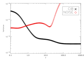
In Fig. 2, we present the variation of the clustered CIB contamination and the reconstructed tSZ map noise level as a function of
the parameter in equation 50. corresponds to the case where we do not account for the clustered CIB
and it leads to large clustered CIB contamination. As expected, the CIB contamination decreases with
as increases. However, as the clustered CIB contamination decreases the noise level increases.
A compromise between noise and clustered CIB contamination can be found for in the range between 3 and 30, as we observe that the noise level is almost constant in this range and the clustered CIB contamination decreases with a slope . Notice that for the
clustered CIB contamination is already reduced by one order of magnitude in variance with respect to the standard ILC algorithm.
On the real data such a compromise can also be found using estimates of both the noise and clustered CIB covariance matrices.
At large values of , we observe that the clustered CIB contamination becomes constant. This behavior is produced by the partial correlation of the clusterd
CIB across frequencies. Indeed, as the CIB emission is not fully correlated between frequencies, it can not be totally removed.
6.3 Characterization of noise level and bias on full-sky simulations
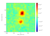
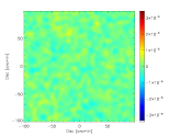
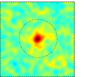
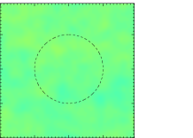
We present in Fig. 3 the reconstructed tSZ map and the residual map in a small patch of 200 by 200 arcmin centered on the well-known pair of clusters A399-A401 (Planck Collaboration Int. VIII, 2013). This example illustrates the ability of MILCA to properly deal with complex tSZ systems like mergers.
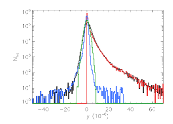
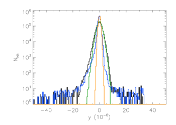
In a more quantitative way we present in Fig. 4 the 1D probability density function (1D pdf) of the reconstructed
MILCA tSZ map for all pixels located inside a radius of 15 arcmin from any of the 1743 clusters of the MCXC catalog Piffaretti et al. (2011).
In the top panel we present the main contributions to the reconstructed tSZ map: tSZ emission (black), noise (green), and other astrophysical components
(blue). For comparison we also plot the input tSZ signal (red). We observe that the reconstructed tSZ map is dominated by the tSZ signal.
In the bottom panel we represent the 1D pdf of the residual map (same color scheme as before).
The residual map is dominated by instrumental noise which contributes to the residual rms at a level of (Compton parameter units),
then, the CIB contributes to a level of and, all other components have a total contribution of about .
Notice in Fig. 4 that most of the residuals by other astrophysical components (in blue) appear as a negative bias, they are mainly produced by radio sources.
An extreme case of such a bias is discussed in Sect. 6.4. We also observe small contamination by IR point sources which appear as positive bias in the reconstructed map. Other astrophysical emissions marginally contribute to the reconstructed signal.
An example of the application of MILCA to real Planck data is presented in Sect. 6.5.
6.4 Empirical extra-constraints for tSZ extraction
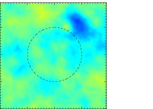
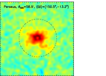
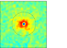
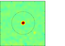
We present an application of MILCA to an extreme case of radio-loud AGN contamination for a simulated Perseus-like cluster.
This particular cluster is well known to be very extended over the sky and to host a radio-loud AGN (Brunzendorf & Meusinger, 1999).
The AGN emission makes the extraction of the tSZ signal for such kind of systems quite complex. However, as the tSZ signal is extended, it is possible to separate the two emissions (from the cluster and from the AGN).
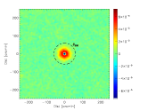
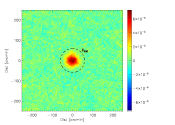
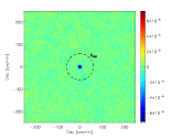
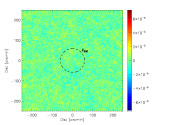
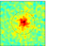
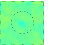
Figure 5 presents the comparison between the tSZ -maps (top) and residuals obtained from a standard ILC adapted to the tSZ effect (left panel) and MILCA (right panel) using three constraints to keep the tSZ signal but removing the CMB and the central radio-loud AGN contamination.
We use an estimate of the AGN SED obtained directly from the data themselves.
For the standard ICL case we observe a strong contamination by the AGN emission (with an amplitude of in Compton parameter units at the center
of the AGN). In this case the tSZ effect and the AGN radio emission are strongly spatially correlated over the sky, leading to the bias discussed in Sect. 4.1, when a correlated component is used to clean the tSZ effect contribution.
When considering an extra constraint, we are able to recover the tSZ signal with a much smaller bias from the AGN (an amplitude of about ). This extra constraint presents however some drawbacks, such as an increase of the noise level (in this case by a factor of 1.5 ) and/or larger bias from other astrophysical un-constrained components.
The ability of MILCA to reduce such contamination is directly related to the accuracy of the estimated SED used for the extra constraint. In order to quantify this we performed simulations of the reconstruction but with an extra-constraint applied on a noisy SED for the AGN
| (69) |
where is the AGN simulated SED, is a random variable following a standard normal distribution and is the relative error on the AGN SED. We performed 200 simulations of reconstruction for a grid of 100 values of .
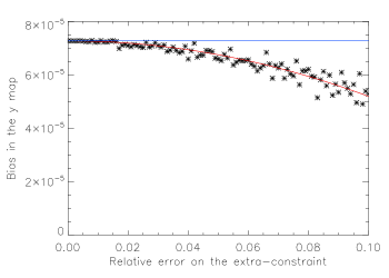
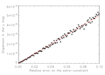
A global bias is computed by averaging the 200 reconstructions and the noise rms is obtained from the standard deviation of the 200 reconstructions. Figure 6 shows the bias and the extra noise induced on the reconstruction by a noisy SED. The bias is proportional to the square of the relative error, , while the extra-noise is directly proportional to . This relation allows us to propagate both bias and noise from the used SED to the final reconstructed map. Notice that the calibration of this relation depends on both the AGN amplitude and the local background of the cluster. Consequently, such estimation of the noise and bias induced by a noisy SED have to be computed for each specific case.
| MILCA | ILC | Residual |
|
|
|
|
|
|
|
|
|
|
|
|
|
|
|
|

|
|

|
|
|
6.5 Extraction of the tSZ effect with MILCA on real data
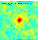
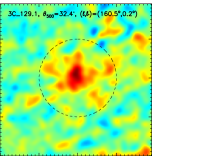
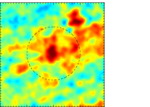
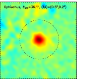
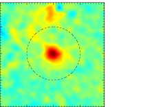
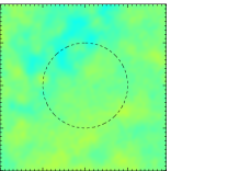
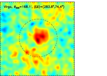
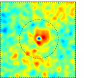
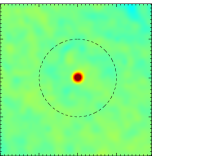
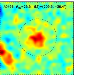
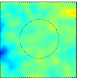
For illustration in Fig. 7, we present tSZ effect reconstructed MILCA (left) maps using the Planck public data for very extended clusters over the sky (see also Planck Collaboration XXIX, 2013). We also present the comparison with a standard ILC reconstruction (middle). These figures illustrate the improvement provided by MILCA for
the reconstruction of tSZ -maps, not only on simulations, but also on real datasets.
For some clusters, such as A2199, Ophiucus and 13627, MILCA and a standard ILC adapted to tSZ extraction produce very similar results. Indeed, for these clusters the foreground contamination is low and not correlated with the tSZ component.
However in the case of AGN contaminated clusters, such as Perseus and Virgo, we observe a clear contamination in the standard ILC maps that is significantly reduced in the MILCA maps. For the Perseus galaxy cluster we observe similar results than the ones obtained on simulated datasets in Sect. 6.4. The use of an extra-constraint allows MILCA to reduce the contamination by radio-loud AGNs, which are correlated to the tSZ effect in the cluster.
For the 3C 129.1 cluster, we observe in the standard ILC map, a large contamination around the tSZ emission. This contamination is mainly produced by thermal dust residuals. This cluster is located in the galactic plane. Consequently, there is a large contamination by dust in this area. However, the MILCA maps are less contaminated by the thermal dust emission. This reduction of the contamination by thermal dust is mainly due to the correction of the noise-induced bias.
Finally for A0496, we observe a reduction of the contamination in MILCA mapbut we still observe contamination by an IR point source. This IR point source is very faint with respect to the thermal dust background. Consequently, it is difficult to extract the SED of this source, reducing the ability of MILCA to minimize the source contamination in the reconstructed tSZ map.
MILCA has been used in the context of the Planck collaboration to produce tSZ -maps for scientific exploitation such as, validation of the catalog of candidates (Planck Collaboration VIII, 2011; Planck Collaboration XXVI, 2011), for the extraction of the cluster pressure profiles (Planck Collaboration Int. V, 2013), for other physicals analysis (Planck Collaboration Int. X, 2012; Planck Collaboration Int. VI, 2013) and for comparison with other experiment (Planck Collaboration Int. II, 2013). MILCA has also been used to produced tSZ maps in Planck Collaboration VIII (2011); Planck Collaboration XXVI (2011) and Planck Collaboration X (2012); Planck Collaboration II (2013); Planck Collaboration VIII (2013); Planck Collaboration XXIX (2013); Planck Collaboration XXI (2013).


7 CO emission reconstruction using the Planck bolometer maps
We present an original application of MILCA for reconstruction of CO emission maps for the first three CO transitions
, and using the spectral mismatch between the bolometers within a single Planck channel
as discussed in Planck Collaboration XIII (2013a).
We discuss here the methodology and performance of the algorithm using the simulations of the Planck 100 GHz channel presented in Sect. 2.
We consider four intensity maps constructed by combining the maps of two bolometers for each of the 4 PSB pairs.
Assuming bolometer maps are calibrated in CMB temperature units we can compute the bandpass mismatch for different astrophysical signals.
For CMB we expect no bandpass mismatch within the calibration uncertainties below 1 %).
For other astrophysical components with a continuous emission spectrum, the variation of transmission in the different bolometers is very small (about 1% at 100GHz).
However, for molecular line associated emission, such as CO, the transmission variations from one bolometer to another can reach up to 20% (Planck Collaboration XIII, 2013a).
Notice that for CMB the transmission variations are null at the calibration uncertainties level.
We use this variation of transmission among bolometers to produce CO maps using MILCA. Formally speaking bandpass mismatch can be
accounted for by assuming a bolometer dependent mixing matrix (rather than one depending on observation frequency) and then component separation algorithms can
be applied. However, there are several problems with this approach. First, spectral bandpass mismatch is very sensitive to the
SED of the astrophysical component and it might be difficult to estimate for those astrophysical components for which the SED vary spatially.
Second, the signal to noise ratio is low with respect to conventional problems based on channel maps.
MILCA is well-adapted for this particular problem as it allow us on the one hand to only use the bandpass mismatch for those components for which is well known
(mainly CMB and the wanted component) and on the other hand to minimize the noise contribution in the final recovered map.
We performed 10 000 simulations of the Planck bolometer maps using different simulated bandpasses based on the CO unit conversion coefficients
values and uncertainties presented in Planck Collaboration XIII (2013a).
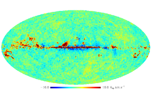
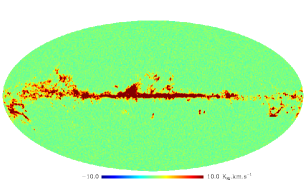
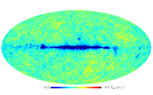
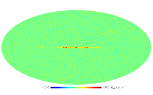
Figure 8 shows the comparison between the reconstructed CO emission at 100 GHz for an ILC algorithm spectrally adapted to CO (left) and for MILCA (right)
for one these simulations. The top panel shows the reconstructed CO map and the bottom panel the residuals in units.
We observe that the CO emission is well reconstructed with MILCA but in the inner Galactic plane where we observe some residual contamination.
However the ILC reconstructed map shows strong contamination by the CMB and the Galactic diffuse emission, and a larger noise level.
In Table 1 we summarize the contamination in terms of contribution to the variance of the CO reconstructed map for MILCA and for the CO adapted ILC.
Notice that MILCA allows us to produce CO maps with a level of contamination 5 times lower than a CO adapted ILC.
At a resolution of 10 arcmin, the MILCA reconstructed CO map residual is dominated by the noise contribution, K.km/s over K.km/s, other components contribute only for K.km/s. For comparison in the ILC CO map the noise contribution is about K.km/s, and the contamination by other components reaches K.km/s.
Also notice that in the case of a MILCA reconstruction at 30 arcmin FWHM, the standard deviation of the map ( K.km/s) is completely dominated by the CO emission (9.11 K.km/s) indicating the high level of purity of the map. For the ILC CO reconstructed map the standard deviation of the total map is K.km/s, which is below the CO only contribution ( K.km/s. This illustrate the large bias in the ILC map for which the thermal dust emission is used to remove CO emission and then to reduce the total variance of the map.
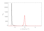
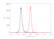
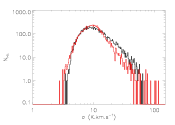
Figure 9 presents the contamination level in the CO map for the 10 000 simulations for the ILC and the MILCA reconstructions. We represent on these figures the contamination by the CMB, the thermal dust + CIB, the tSZ effect and the synchrotron + free-free + radio point sources and by the noise.
For CMB, the contamination in MILCA map is equal to zero at the calibration uncertainties level, but in the ILC map we observe a large contamination by the CMB, which accounts to 2.5 K.km/s in average in terms of the standard deviation.
This contamination is mainly produced by the CO/galactic foregrounds correlation. Indeed the galactic foregrounds with a continuous emission law follow almost the same spectral dependence in the different bolometers than the CMB. Consequently, we observe similar residuals for all contaminating astrophysical emission at the percents level. The bias in the ILC map is mainly driven by the CO/thermal dust correlation, as the distribution of the dust contamination is the tightest.
| Maps | CO ILC () | CO ILC () |
|---|---|---|
| Total | 10.43 | 5.94 |
| CO | 10.16 | 9.11 |
| Residuals | 9.36 | 4.64 |
| Noise | 7.55 | 0.57 |
| Other components | 5.53 | 4.60 |
| CMB | 1.45 | 1.14 |
| Dust + CIB | 5.02 | 4.16 |
| Sync + Free-Free | 0.50 | 0.46 |
| SZ | 0.025 | 0.017 |
| Maps | CO MILCA () | CO MILCA () |
| Total | 12.05 | 9.35 |
| CO | 10.16 | 9.11 |
| Residuals | 6.07 | 0.53 |
| Noise | 6.06 | 0.46 |
| Other components | 0.31 | 0.25 |
| CMB | 0 | 0 |
| Dust + CIB | 0.35 | 0.29 |
| Sync + Free-Free | 0.08 | 0.07 |
| SZ | 0.0020 | 0.0013 |
MILCA have been applied to the Planck bolometer maps at 100, 217 and 353 GHz in order to extract maps of the emission of the first three CO lines J=1-0, J=2-1 and J=3-2 (Planck Collaboration XIII, 2013a). These maps were released by the Planck collaboration and have extensively been compared with external data in Planck Collaboration XIII (2013a).
8 Conclusion
Component separation techniques are now a major ingredient in the scientific exploitation of
multi-channel and multi-component datasets as those of the CMB satellite experiments WMAP and Planck.
In this paper we have presented the Modified Internal Linear Algorithm (MILCA) specially developed for the Planck data.
MILCA generalizes the standard ILC algorithm, generally devoted to CMB emission extraction, to any astrophysical component with a known emission law.
In practice MILCA can be used to extract an arbitrary number of astrophysical emissions rejecting the contribution from others for which the
emission law is also known. MILCA has been optimized in various ways in order to reduce significantly residuals from instrumental noise and
other astrophysical components. For this purpose the separation is performed both in real and Fourier spaces. Moreover
the data covariance matrix is modified and divided into multiple subspaces in order to avoid the confusion
between instrumental noise and astrophysical components in the original data. Finally, we have also introduced the possibility of using external
templates to improve the efficiency of the algorithm. Because of these improvements MILCA has been proved to be
more efficient than standard ILC algorithms in a large range of astrophysical problems.
We have applied MILCA to simulated Planck data, and have shown that it can be used to efficiently reconstruct the tSZ and CO emissions.
We have proposed, with MILCA, an original way to used prior on the spatial distribution of contaminating components. Allowing to constraint emissions such as CIB, which can not be described with a single template and an SED.
In the tSZ case we have showed that MILCA can be used to reconstruct low signal to noise and highly non-Gaussian components in the Planck
data. Indeed, MILCA has been used extensively by the Planck collaboration for tSZ studies (Planck Collaboration VIII, 2011; Planck Collaboration XXVI, 2011; Planck Collaboration Int. V, 2013; Planck Collaboration Int. X, 2012; Planck Collaboration Int. VI, 2013; Planck Collaboration XXIX, 2013; Planck Collaboration XXI, 2013). For CO emission we have presented a new component separation approach that takes advantage of the spectral bandpass mismatch between
bolometers of the same Planck channel. We have proved that MILCA improvements on the reduction of the instrumental noise and unwanted astrophysical
components are critical for this. Maps of the emission for the first three CO transitions have been obtained by the Planck collaboration using MILCA (Planck Collaboration XIII, 2013a).
Acknowledgements
We thank Nabila Aghanim and François-Xavier Désert for useful discussions related to this work. Some of the results in this paper have been derived using the HEALPix package (Górski et al., 2005).
References
- Addison et al. (2012) Addison, G. E., Dunkley, J., & Spergel, D. N. 2012, MNRAS, 427, 1741
- Arnaud et al. (2010) Arnaud, M., Pratt, G. W., Piffaretti, R., et al. 2010, A&A, 517, A92
- Aumont & Macías-Pérez (2007) Aumont, J. & Macías-Pérez, J.-F. 2007, MNRAS, 376, 739
- Basak & Delabrouille (2012) Basak, S. & Delabrouille, J. 2012, MNRAS, 419, 1163
- Bennett et al. (1996) Bennett, C. L., Banday, A. J., Gorski, K. M., et al. 1996, ApJ, 464, L1
- Bennett et al. (2003) Bennett, C. L., Halpern, M., Hinshaw, G., et al. 2003, ApJS, 148, 1
- Bersanelli et al. (2010) Bersanelli, M., Mandolesi, N., Butler, R. C., et al. 2010, A&A, 520, A4+
- Bobin et al. (2008) Bobin, J., Moudden, Y., J.-L., S., J., F., & Aghanim, N. 2008, Statistical Methodology, 5, 307
- Bobin et al. (2013) Bobin, J., Starck, J.-L., Sureau, F., & Basak, S. 2013, A&A, 550, A73
- Bonaldi et al. (2006) Bonaldi, A., Bedini, L., Salerno, A., Baccigalupi, C., & de Zotti. 2006, MNRAS, 373, 271
- Brunzendorf & Meusinger (1999) Brunzendorf, J. & Meusinger, H. 1999, A&AS, 139, 141
- Cardoso et al. (2008) Cardoso, J.-F., Le Jeune, M., Delabrouille, J., Betoule, M., & Patanchon, G. 2008, IEEE Journal of Selected Topics in Signal Processing, 2, 735
- Dame et al. (2001) Dame, T. M., Hartmann, D., & Thaddeus, P. 2001, ApJ, 547, 792
- Davies et al. (1996) Davies, R. D., Watson, R. A., & Gutierrez, C. M. 1996, MNRAS, 278, 925
- Delabrouille et al. (2003) Delabrouille, J., Cardoso, J.-F., & Patanchon, G. 2003, MNRAS, 346, 1089
- Desert et al. (1990) Desert, F.-X., Boulanger, F., & Puget, J. L. 1990, A&A, 237, 215
- Dick et al. (2010) Dick, J., Remazeilles, M., & Delabrouille, J. 2010, MNRAS, 401, 1602
- Dickinson et al. (2003) Dickinson, C., Davies, R. D., & Davis, R. J. 2003, MNRAS, 341, 369
- Eriksen et al. (2004) Eriksen, H. K., Banday, A. J., Górski, K. M., & Lilje, P. B. 2004, ApJ, 612, 633
- Eriksen et al. (2008) Eriksen, H. K., Jewell, J. B., Dickinson, C., et al. 2008, ApJ, 676, 10
- Finkbeiner (2003) Finkbeiner, D. P. 2003, ApJS, 146, 407
- Górski et al. (2005) Górski, K. M., Hivon, E., Banday, A. J., et al. 2005, ApJ, 622, 759
- Haslam et al. (1981) Haslam, C. G. T., Klein, U., Salter, C. J., et al. 1981, A&A, 100, 209
- Hinshaw et al. (2003) Hinshaw, G., Spergel, D. N., Verde, L., et al. 2003, ApJS, 148, 135
- Hinshaw et al. (2009) Hinshaw, G., Weiland, J. L., Hill, R. S., et al. 2009, ApJS, 180, 225
- Hobson et al. (1998) Hobson, M. P., Jones, A. W., Lasenby, A. N., & Bouchet, F. R. 1998, MNRAS, 300, 1
- Lamarre et al. (2010) Lamarre, J., Puget, J., Ade, P. A. R., et al. 2010, A&A, 520, A9+
- Maino et al. (2002) Maino, D., Farusi, A., Baccigalupi, C., & et al. 2002, MNRAS, 334, 53
- Mennella et al. (2011) Mennella, A., Butler, R. C., Curto, A., et al. 2011, A&A, 536, A3
- Miville-Deschênes & Lagache (2005) Miville-Deschênes, M.-A. & Lagache, G. 2005, ApJS, 157, 302
- Piffaretti et al. (2011) Piffaretti, R., Arnaud, M., Pratt, G. W., Pointecouteau, E., & Melin, J.-B. 2011, A&A, 534, A109
- Planck Collaboration I (2011) Planck Collaboration I. 2011, A&A, 536, A1
- Planck Collaboration I (2013) Planck Collaboration I. 2013, Submitted to A&A, arXv:1303.5062
- Planck Collaboration II (2013) Planck Collaboration II. 2013, A&A, 550, A128
- Planck Collaboration Int. II (2013) Planck Collaboration Int. II. 2013, A&A, 550, A128
- Planck Collaboration Int. V (2013) Planck Collaboration Int. V. 2013, A&A, 550, A131
- Planck Collaboration Int. VI (2013) Planck Collaboration Int. VI. 2013, A&A, 550, A132
- Planck Collaboration Int. VII (2013) Planck Collaboration Int. VII. 2013, A&A, 550, A133
- Planck Collaboration Int. VIII (2013) Planck Collaboration Int. VIII. 2013, A&A, 550, A134
- Planck Collaboration Int. X (2012) Planck Collaboration Int. X. 2012, ArXiv e-prints
- Planck Collaboration VII (2011) Planck Collaboration VII. 2011, A&A, 536, A7
- Planck Collaboration VIII (2011) Planck Collaboration VIII. 2011, A&A, 536, A8
- Planck Collaboration VIII (2013) Planck Collaboration VIII. 2013, A&A, 550, A134
- Planck Collaboration X (2012) Planck Collaboration X. 2012, ArXiv e-prints
- Planck Collaboration XIII (2011) Planck Collaboration XIII. 2011, A&A, 536, A13
- Planck Collaboration XIII (2013a) Planck Collaboration XIII. 2013a, ArXiv e-prints
- Planck Collaboration XIII (2013b) Planck Collaboration XIII. 2013b, Submitted to A&A, arXv:1303.5090
- Planck Collaboration XV (2013) Planck Collaboration XV. 2013, ArXiv e-prints
- Planck Collaboration XVI (2013) Planck Collaboration XVI. 2013, ArXiv e-prints
- Planck Collaboration XVIII (2011) Planck Collaboration XVIII. 2011, A&A, 536, A18
- Planck Collaboration XX (2011) Planck Collaboration XX. 2011, A&A, 536, A20
- Planck Collaboration XXI (2013) Planck Collaboration XXI. 2013, ArXiv e-prints
- Planck Collaboration XXIX (2013) Planck Collaboration XXIX. 2013, Submitted to A&A, arXv:1303.5089
- Planck Collaboration XXVI (2011) Planck Collaboration XXVI. 2011, A&A, 536, A26
- Planck HFI Core Team (2011) Planck HFI Core Team. 2011, A&A, 536, A4
- Remazeilles et al. (2011) Remazeilles, M., Delabrouille, J., & Cardoso, J.-F. 2011, MNRAS, 410, 2481
- Smoot et al. (1992) Smoot, G. F., Bennett, C. L., Kogut, A., et al. 1992, ApJ, 396, L1
- Stolyarov et al. (2002) Stolyarov, V., Hobson, M. P., Ashdown, M. A. J., & Lasenby, A. N. 2002, MNRAS, 336, 97
- Sunyaev & Zeldovich (1972) Sunyaev, R. A. & Zeldovich, Y. B. 1972, Comments on Astrophysics and Space Physics, 4, 173
- The Planck Collaboration (2006) The Planck Collaboration. 2006, ArXiv Astrophysics e-prints
- Vio & Andreani (2008) Vio, R. & Andreani, P. 2008, A&A, 487, 775