Baryon fractions in clusters of galaxies: evidence against a preheating model for entropy generation
Abstract
The Millennium Gas project aims to undertake smoothed-particle hydrodynamic resimulations of the Millennium Simulation, providing many hundred massive galaxy clusters for comparison with X-ray surveys (170 clusters with keV). This paper looks at the hot gas and stellar fractions of clusters in simulations with different physical heating mechanisms. These fail to reproduce cool-core systems but are successful in matching the hot gas profiles of non-cool-core clusters. Although there is immense scatter in the observational data, the simulated clusters broadly match the integrated gas fractions within . In line with previous work, however, they fare much less well when compared to the stellar fractions, having a dependence on cluster mass that is much weaker than is observed. The evolution with redshift of the hot gas fraction is much larger in the simulation with early preheating than in one with continual feedback; observations favour the latter model. The strong dependence of hot gas fraction on cluster physics limits its use as a probe of cosmological parameters.
keywords:
methods: N-body simulations – galaxies: clusters: general – galaxies: evolution1 Introduction
The hot gas fraction of clusters of galaxies was first used as a cosmological probe by Allen et al. (2002), and later refined in Allen et al. (2004) and Allen et al. (2008). These papers show quite conclusively that the gas fraction can be used to derive cosmological parameters that are in agreement with the concordance CDM cosmology. A similar result was obtained by LaRoque et al. (2006) in a joint X-ray, Sunyaev-Zel’dovich analysis. Subsequently, a more sophisticated analysis that properly takes into account selection effects, and combines mass, X-ray luminosity and temperature observations of 238 clusters at , reached similar conclusions (Mantz et al., 2009a, b), as did a study by Ettori et al. (2009) of 60 clusters extending to .
However, as has been pointed out by Sadat et al. (2005), the above conclusion relies very heavily upon the assumption that the gas fraction in the clusters used in the study is independent of both mass and redshift. We show in this paper that using different models for entropy generation in the intracluster medium (ICM) can lead to variations in hot gas fractions in simulated clusters that are at least as great as those that one obtains by using an incorrect cosmology in the observational data analysis. We argue, therefore, that, at present, it is more useful to fix the cosmology to the concordance value and to use the data to constrain cluster physics. By doing so we conclude that the data favour a model of continual energy injection into the ICM from galaxies rather than a widespread preheating episode at high redshift.
In the future, once the physical models of the ICM become more refined, and with the large statistical samples of clusters generated by eROSITA, it should be possible to do a combined analysis that constrains both the cluster physics and the cosmology simultaneously.
In Section 2 we describe the numerical method that we use, the different feedback schemes, and our method of cluster identification. Section 3 describes our results first on gas fraction profiles, then scaling relations, and finally the evolution of each of these. The conclusions of the paper are summarised in Section 4.
2 Method
Here we present an overview of our numerical scheme. The method is described at length in Short & Thomas (2009) and its particular application to clusters of galaxies in Short et al. (2010).
2.1 Simulations
We present results from three simulations taken from the Millennium Gas Project, the basic objective of which is to add gas to the dark matter-only Millennium Simulation (Springel et al., 2005). Each simulation incorporates a different model of the baryonic physics, so that we can assess the impact of varying physical assumptions on the thermal history of the ICM.
In the first Millennium Gas run, the intracluster gas is heated solely by gravitational processes. We refer to this simulation as the GO (Gravitation Only) run. Although this run does not include gas cooling or heating from astrophysical sources such as supernovae (SNe) and active galactic nuclei (AGN), it is useful as a base model, enabling us to determine exactly which cluster properties are affected by astrophysical processes beyond gravitational heating. Given that the only source of gas entropy changes in the GO run is gravity, then we would expect a self-similar cluster population to be formed. This is generally found to be the case in non-radiative simulations (e.g. Navarro et al. 1995; Eke et al. 1998; Voit et al. 2005; Ascasibar et al. 2006; Muanwong et al. 2006; Stanek et al. 2010).
The second Millennium Gas simulation also includes high-redshift preheating (first posited by Kaiser, 1991; Evrard & Henry, 1991) and radiative cooling. We name this simulation the PC (Preheating plus Cooling) run. Preheating raises the entropy of the ICM before gravitational collapse, preventing gas from reaching high densities in central cluster regions and thus reducing its X-ray emissivity. This effect is greater in lower-mass systems, breaking the self-similarity of the cluster scaling relations in a way that resembles observations (Bialek et al., 2001; Brighenti & Mathews, 2001; Muanwong et al., 2002; Borgani et al., 2002; Tornatore et al., 2003; Borgani et al., 2005).
The simple model of preheating employed in the PC simulation is similar to that of Borgani et al. (2002). Briefly, the entropy of every particle is raised to keV cm2 at , thus creating an entropy ‘floor’ (note that a particle’s entropy is not changed if it already has a value in excess of this at ). In addition to preheating, there is also radiative cooling based on the cooling function of Sutherland & Dopita (1993), assuming a fixed metallicity of (a good approximation to the mean metallicity of the ICM out to at least ; Tozzi et al. 2003). Once the temperature of a gas particle drops below K, the hydrogen density exceeds g cm-3 and the density contrast is greater than , then it is converted to a collisionless star particle. However, the preheating is so extreme that star formation is effectively terminated at , so that less than of the baryonic matter is locked-up in stars at .
Although there is considerable evidence that non-gravitational heating of the ICM indeed occurs mainly at high redshift (e.g. Eisenhardt et al. 2008; Weiner et al. 2009), the preheating scenario is clearly a gross simplification of the complex interplay between star formation, black hole growth and associated feedback. Despite this, preheating does provide a useful effective model for the effects of non-gravitational heating. In particular, the Millennium Gas PC run can reproduce several key observational properties of the low-redshift cluster population, including halo gas fractions (Stanek et al., 2010). However, the model fails to account for the observed scatter about the mean relations, particularly on group scales, and generates over-large isentropic cores in low-mass systems as compared to observational data (e.g. Ponman et al. 2003; Pratt et al. 2006).
Finally, we use a recent addition to the Millennium Gas suite in which feedback is directly tied to galaxy formation, rather than assuming some ad hoc injection of energy at high-redshift. We term this the FO (Feedback Only) run to emphasise the fact that the model currently does not include radiative cooling. The model we use is the hybrid scheme of Short & Thomas (2009), where a semi-analytic model is used to calculate the energy transferred to the intracluster gas by SNe and AGN. An immediate benefit of this approach is that feedback is guaranteed to originate from a galaxy population whose observational properties agree well with those of real galaxies. This is generally not the case in fully self-consistent hydrodynamical simulations that include radiative cooling and stellar feedback because too much gas cools out of the hot phase, leading to excessive star formation (e.g. Borgani et al. 2004; Kay et al. 2007a). It is widely thought that additional heating from AGN is the natural solution to this overcooling problem. Indeed, McCarthy et al. (2009) and Fabjan et al. (2010) have demonstrated that including AGN feedback in hydrodynamical simulations can successfully balance radiative cooling in galaxy groups. However, the stellar fraction is still found to be 2 to 3 times larger than observed in massive clusters.
For reasons of computational efficiency, the FO run was not undertaken over the entire Millennium Simulation volume. Instead, we resimulated a sample of several hundred galaxy groups and clusters. Each run came in three distinct stages: a dark matter-only resimulation of each region containing a cluster from our sample; semi-analytic galaxy catalogues built on the halo merger trees of these resimulations; and hydrodynamical resimulations of the same regions to track the energy injection from model galaxies. The merger trees were built using the procedure of Springel et al. (2005) and we used the Munich L-Galaxies semi-analytic model with the same parameters as described in De Lucia & Blaizot (2007). Energy is injected into the ICM from both SNe and AGN following the prescription of Short & Thomas (2009). The procedure is described in full in Short et al. (2010)
By coupling a SAM to a hydrodynamical simulation, Short & Thomas (2009) showed that their hybrid feedback model could reproduce the observed mean - relation for groups and poor clusters at , but only if there was a large energy input into the ICM from AGN over the entire formation history of halos. The AGN heating is efficient at driving X-ray emitting gas from the central regions of low-mass halos, reducing their luminosity and steepening the - relation as desired. Unlike the simple preheating scenario, their model was also able to account for some of the scatter about the mean relation seen for temperatures keV, attributable to the varied merger histories of groups. In addition, the gas fractions of their simulated groups and poor clusters were found to broadly agree with observational data, rapidly declining at low temperatures and exhibiting a comparable amount of scatter.
The main limitation of both the PC and the FO simulations is that neither can reproduce the low entropy found in the centres of cool-core clusters. For the FO run this is because cooling is not incorporated in the hydrodynamical simulations; whereas in the PC run preheating expels gas from cluster cores at high redshift, limiting the subsequent cooling.
The cosmological model adopted in all three Millennium Gas simulations is a spatially-flat CDM model with parameters , , , , and . Here , and are the total matter, baryon and dark energy density parameters, respectively, is the Hubble parameter in units of km s-1 Mpc-1, is the spectral index of primordial density perturbations, and is the rms linear density fluctuation within a sphere of radius Mpc. The subscript signifies the value of a quantity at the present day. These cosmological parameters are the same as those used in the original Millennium simulation and are consistent with a combined analysis of the first-year Wilkinson Microwave Anisotropy Probe (WMAP) data (Spergel et al., 2003) and data from the Two-degree-Field Galaxy Redshift Survey (Colless et al., 2001). However, there is some tension between the chosen parameter values, particularly and , and those derived from the seven-year WMAP data (Komatsu et al., 2010). More significantly for this paper, the mean value of the baryon density, , is higher than the WMAP 7-year value of .
2.2 Cluster catalogues
Cluster catalogues are generated at several redshifts for the three Millennium Gas simulations using a procedure similar to that employed by Muanwong et al. (2002). Essentially, a friend-of-friends algorthm is used to identify peaks in the density field and then spheres are grown around these peaks until they enclose regions of a given overdensity.
We define overdensity, , with respect to the critical density, , at any given redshift,
| (1) |
where is the mean density within radius , is the mass within this region and is the gravitational constant. We express our masses in units of , rescaling observational data to this system when required.
Low-mass clusters are more affected by non-gravitational heating processes than high-mass ones. Observationally, temperature is often used as a proxy for mass as the two are strongly correlated. For that reason, we often divide the clusters into bins according to their spectroscopic-like temperature, , defined as
| (2) |
where is the gas density, the physical temperature, and the integral runs over volume. Mazzotta et al. (2004) have shown to be a good approximation to the temperature recovered by X-ray spectral analysis software in the bremsstrahlung regime.
The scaling relations for the GO and PC runs can be dominated by small objects. For this reason, we remove many clusters from our sample such that the remaining clusters are distributed evenly in , with a lower mass-limit that corresponds to 1000 particles each of gas and dark matter within . For the FO run we resimulate all clusters with keV and a selection of clusters below this temperature, again chosen evenly in . This has a much higher mass resolution and so the lower mass limit in this case, , was instead fixed by the total number of clusters that we wish to simulate. When plotting as a function of mass at an overdensity other than the one used in the selection procedure, there will not be a clean lower mass-limit; however this is a very minor effect that does not lead to any significant bias in our results.
3 Results
In this section we first discuss the radial profiles of the hot gas fractions of clusters at the present day. We then characterise the dependence of the hot gas fraction upon cluster mass, and investigate the scatter about that mean relation. Finally, we look at the variation of the hot gas fraction with redshift.
3.1 Profiles
3.1.1 Differential hot gas profiles
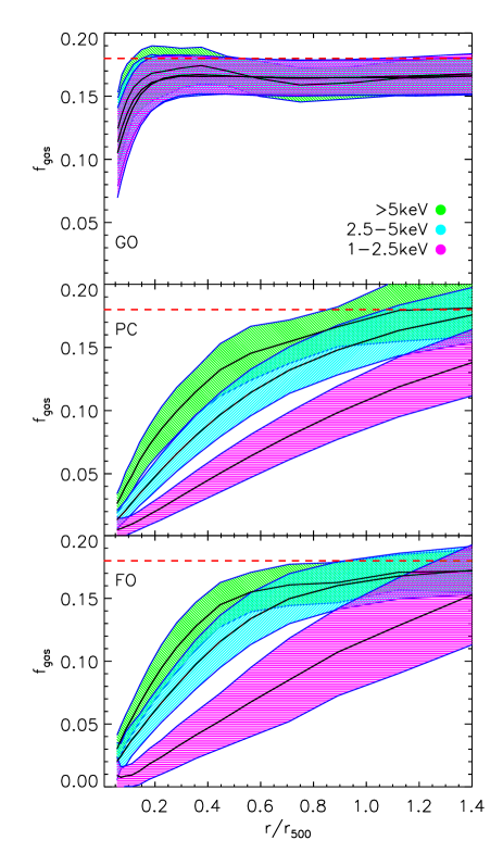
Figure 1 shows the differential gas mass fraction profiles for clusters in three temperature ranges, keV (upper, green regions), 2.5 keV 5 keV (middle, cyan regions) and 2.5 keV (lower, magneta regions). The curves are plotted out to beyond (the radius at which ), which is the region accessible to X-ray observations.
For the GO run the gas fraction plateaus at a value of 0.16–0.17 at about , although there is a very slow increase at larger radii (beyond the right-hand edge of the plot). This is less than the global baryon fraction of 0.18: conversion of kinetic energy into heat, together with continual stirring of the gas by the motion of dark matter structures, allows the gas to pick up energy at the expense of the dark matter (e.g. Pearce et al., 1994). This is particularly evident in the cluster cores: for the largest clusters, is of order 1 Mpc; therefore the drop in baryon fraction in the core of the clusters occurs on a scale significantly larger than the force softening (25 kpc).
In the PC and FO runs, gas has been expelled from the cluster cores and pushed to larger radii. The effect is more pronounced at lower masses: thus the gas profiles of clusters with keV are still steeply rising at , while for keV the profiles are approximately constant beyond this radius. The inconstancy of the gas fraction is both a nuisance, requiring careful calibration before we can use clusters as cosmological probes, and a useful test of any model of entropy generation in the ICM.
3.1.2 Comparison with observations
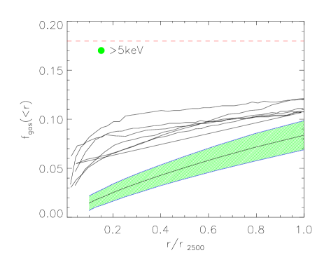
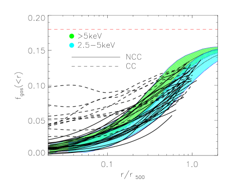
Rather than plotting differential profiles, observational studies tend to report the cumulative gas fractions, averaged within some radius. Figure 2 shows the cumulative gas fraction profiles in the FO run compared to several different observational studies (Vikhlinin et al., 2006; Allen et al., 2008; Pratt et al., 2010). We have only plotted simulated clusters in temperature ranges corresponding to those of the various observational data sets. To save space, we do not show the results from the PC run—these are similar.
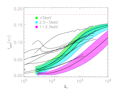
All three observational studies plot the gas fractions using a different ordinate. The top panel, from Vikhlinin et al. (2006), uses overdensity relative to the critical density. They looked at 13 Chandra clusters with a range of temperatures upwards of about 1.5 keV for which the data extend out to large radii. The simulated and observed clusters agree at the outer limit of the data, but the former fall more rapidly as one moves into the cluster centre.
The middle panel shows data from Allen et al. (2008). They again study Chandra clusters, but they focus on the inner regions of 42 hot ( keV) systems. As can clearly be seen, the simulated clusters lie well below the observations within .
Both the above studies focus on bright, relaxed systems (those that are likely to be labelled cool core, or CC). By way of contrast, the REXCESS survey (Böhringer et al., 2007; Pratt et al., 2010), shown in the lower panel of Figure 2, is sample of 33 nearby galaxy clusters from XMM-Newton, selected so as to sample a broad range of luminosities and with no bias towards any morphological type. The temperature range here is 2-9 keV with the more massive clusters lying towards the upper edge of the observed band, and the least massive ones towards the bottom. Here the simulations are much more successful in reproducing the observed profiles, providing a fair match to the non-cool-core (NCC) population out to the limit of the observations. They fail to reproduce CC clusters (those with flattened baryon fraction profiles in their inner regions), however these are much less frequent than in the relaxed samples.
We conclude that our simulated clusters provide a fair match to the hot gas fractions in typical NCC clusters, but fail to reproduce the higher gas fractions seen in the central regions of the brighter, CC clusters.
The results for our adiabatic halos agree with other previous simulations undertaken with SPH (e.g. Kravtsov et al., 2005; Ettori et al., 2006; Crain et al., 2007). Direct comparison of the other runs is more difficult because we use different feedback models.
Qualitatively, we see a similar behaviour in the profiles of the hot gas fraction to previous work, but the baryon fraction profile is very different in our FO run because of the much reduced stellar fraction. The integrated baryon fractions within are considered in Section 3.2.3.
3.2 Scaling relations
3.2.1 Cumulative hot gas fractions
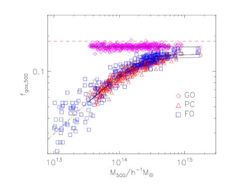
Figure 3 shows the cumulative gas fraction within a radius of as a function of total mass. The GO points are consistent with a constant value of 0.162, slightly smaller than the universal mean of 0.18. By contrast, both the PC and the FO runs have hot gas fractions that are strong functions of mass, because the feedback processes are more effective in lower-mass clusters and evacuate more of the gas.
Figure 4 contrasts the hot gas fractions for the FO run within three different radii corresponding to enclosed overdensities of , , and (the PC run gives similar results). In each case the mass has been measured within the corresponding radius. As expected from the radial profiles, the gas fraction is an increasing function of scale radius (i.e. decreasing overdensity). Note that, for a fixed enclosed mass, the variation in enclosed gas fraction is relatively modest: e.g. at it varies from 0.07 for to 0.10 for . This is much less than the variation seen if a fixed overdensity is used to measure the mass, e.g. for , the enclosed gas fraction increases from 0.04 to 0.11 as the overdensity drops from 2500 to 200.
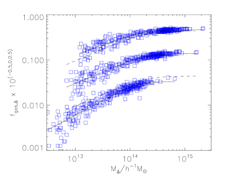
In Figures 3 and 4, we fit the hot gas fraction scaling relations with models of the form
| (3) |
where and , , and are fitting parameters. In log space, this represents a line of constant slope, , at masses well below , bending over to a constant value of at high masses. For low enclosed overdensities we would expect to tend towards the universal baryon fraction of 0.18, although we do not impose this as a constraint. is a parameter that controls the abruptness of the transition between the two regimes. The data are not always sufficient to independently constrain all the parameters, and in particular : for that reason we use a fixed value of when recording our fits. The best-fit models are shown as solid lines in the figures, and the parameters are listed in Table 1, along with the scatter about the best-fit relation.
| Model | Overdensity | ||||
|---|---|---|---|---|---|
| GO | 2500 | 0.158 | 0.036 | ||
| 500 | 0.161 | 0.018 | |||
| 200 | 0.163 | 0.013 | |||
| 5002500 | 0.164 | 0.026 | |||
| 200500 | 0.166 | 0.033 | |||
| PC | 2500 | 0.103 | 14.15 | 0.590 | 0.048 |
| 500 | 0.134 | 14.26 | 0.519 | 0.041 | |
| 200 | 0.150 | 14.43 | 0.363 | 0.027 | |
| 5002500 | 0.161 | 14.28 | 0.393 | 0.037 | |
| 200500 | 0.180 | 14.10 | 0.263 | 0.044 | |
| FO | 2500 | 0.126 | 14.25 | 0.650 | 0.124 |
| 500 | 0.143 | 14.26 | 0.552 | 0.061 | |
| 200 | 0.148 | 14.21 | 0.472 | 0.058 | |
| 5002500 | 0.163 | 14.13 | 0.492 | 0.076 | |
| 200500 | 0.173 | 13.72 | 0.512 | 0.066 |
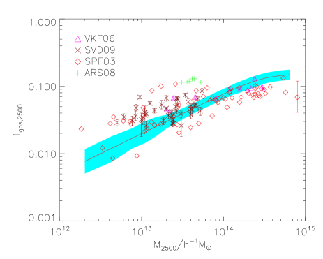
Figure 5 shows the cumulative hot gas fractions in the FO run within and as a function of mass. The shaded region shows the 1-sigma spread about the mean relation from the simulation and the points are observational data from the sources listed in the figure caption. Concentrating first on the upper panel, it is apparent that there are systematic differences in the reported hot-gas fractions that cannot be attributed solely to statistical error. In particular, the Allen et al. (2008) data lie significantly above those of the other studies. This may be because they concentrated on regular, CC clusters that are likely to lie up the upper edge of the distribution. Even given these observational inconsistencies, however, the simulations show a much greater variation in gas fraction with than do the observations. It would seem that in the FO run (and the PC run is similar) we have ejected too much material from within this radius in small clusters, and too little in large ones.
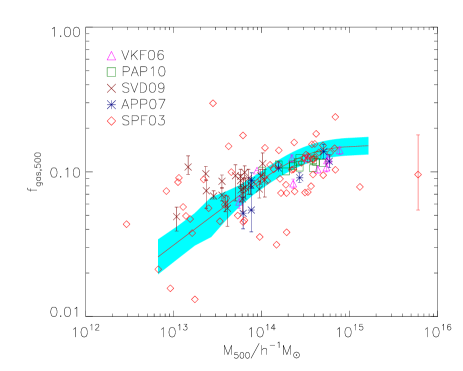
Moving out to , as shown in the lower panel of the figure, the simulations and observations are in better agreement. There is again a suggestion that the observational data would prefer higher gas fractions than the simulations below a cluster mass of of , but the scatter in the observational measurements is large. At higher masses, the two show a similar trend of increasing gas fraction with cluster mass, although the simulated values are perhaps slightly too high. This is presumably because the mean baryon fraction that we have used in the simulations, 0.18, is higher than the current WMAP best fit value of 0.168.
3.2.2 Differential hot gas fractions
The profiles of Figure 1 suggest that the differential gas fraction between radii of and may provide a measure that is more independent of mass than the cumulative gas fractions of the previous section.
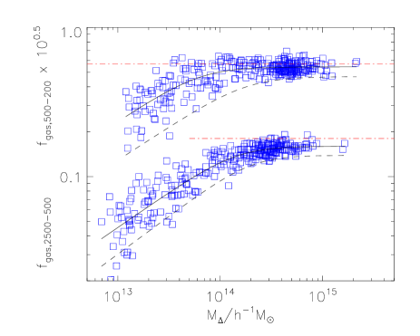
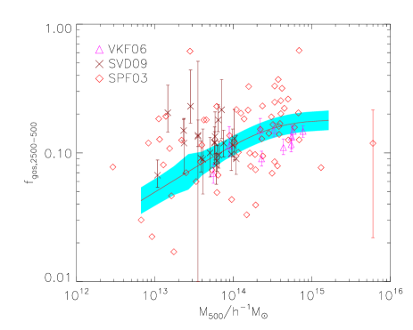
In Figure 6 we show differential gas fractions, - and -, for the FO model (once again, the PC run gives similar results). Both are higher than the equivalent cumulative measures, although the universal gas fraction is reached only for the most massive clusters () at radii . Clearly the differential gas fraction at larger radii, –, is more nearly constant and so provides the more accurate probe of cosmology, but observationally the inner annulus, –, provides a compromise between eliminating the depleted inner region and having enough counts to enable a reliable X-ray determination of the gas density. The observational data from Sanderson et al. (2003), Vikhlinin et al. (2006) and Sun et al. (2009), plotted in Figure 7, present a confused picture. The Sanderson et al. (2003) data broadly mimic the simulations, but the statistical scatter in their data is very large. Vikhlinin et al. (2006) report the smallest error bars for their data and find differential gas fractions that increase strongly with mass, but which lie below the simulated values; whereas, at lower masses, the Sun et al. (2009) data seem to require hot gas fractions that are decreasing, or at best flat, as a function of mass. We conclude that these differential measurements are not yet sufficiently robust to provide useful constraints.
It is interesting to note that both the PC and FO models have higher differential gas fractions at large radii than does the GO model. The injection of entropy has removed gas from the cores of the clusters and pushed it out to larger radii, between and . In a steady-state, the higher entropy in these runs would ensure that they have a lower gas density than in the GO model: we conclude that on large scales, although still within the virial radius, the clusters are not in dynamical equilibrium.
3.2.3 Baryon fractions
The baryon fractions are also well-fit by the model given in Equation 3 with parameters as listed in Table 2. Because clusters are large systems with deep potential wells, it is often stated that they should enclose a representative sample of the Universe, and in particular that they should contain the Universal fraction of baryons. Indeed, we find this is approximately true, with only a small baryon deficit within .
| Model | Overdensity | ||||
|---|---|---|---|---|---|
| PC | 2500 | 0.141 | 14.32 | 0.250 | 0.061 |
| 500 | 0.161 | 14.44 | 0.307 | 0.037 | |
| 200 | 0.168 | 14.49 | 0.271 | 0.030 | |
| 5002500 | 0.174 | 14.29 | 0.362 | 0.035 | |
| 200500 | 0.188 | 14.10 | 0.269 | 0.042 | |
| FO | 2500 | 0.156 | 14.92 | 0.251 | 0.069 |
| 500 | 0.150 | 14.48 | 0.308 | 0.052 | |
| 200 | 0.157 | 14.41 | 0.291 | 0.044 | |
| 5002500 | 0.167 | 14.25 | 0.357 | 0.053 | |
| 200500 | 0.181 | 13.94 | 0.333 | 0.058 |
Observationally, the baryon fraction is hard to determine because of the difficulty in measuring the contribution from dwarf galaxies and from intracluster light (stars that have been stripped from galaxies). This latter component may comprise as much as 40 percent of the total light of the cluster (Bernstein et al., 1995; Gonzalez et al., 2000; Feldmeier et al., 2002, 2004; Gonzalez et al., 2005; Krick et al., 2006; Zibetti et al., 2005). Except for the brightest X-ray clusters, the measurement of total mass is also problematic.
Gonzalez et al. (2007, hereafter GZZ07), in a sample of 12 groups and clusters spanning a wide mass range, find that the baryon fraction is independent of mass and averages to 0.133 within . Laganá et al. (2008, hereafter LLA08) with a smaller sample of 5 high-mass clusters find a slightly lower value of 0.123 (the mean of their quoted numbers, weighted by the inverse square of their errors). On the other hand Giodini et al. (2009, hereafter GPF09), in a sample of 41 clusters drawn from Vikhlinin et al. (2006), Arnaud et al. (2007) and Sun et al. (2009), find that the baryon fraction is a slowly-increasing function of mass. The baryon fractions for our FO and PC clusters are compared to these observations in Figure 8
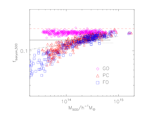
The observations and the simulations approximately agree for cluster masses of 1–. However the simulations show a strong variation with cluster mass, even more so than that of GPF09. This difference is attributable mainly to differences in star formation, as described below.
3.2.4 Stellar fractions
Both our PC and our FO models have much more modest star formation than do many previous simulations (e.g. Borgani et al., 2004; Ettori et al., 2006; Kay et al., 2007a; Nagai et al., 2007; Davé et al., 2008; Fabjan et al., 2010; Puchwein et al., 2010). In particular, the FO run takes its star-formation rate from the highly-successful L-Galaxies semi-analytic model. The mean stellar fraction in our high mass clusters in the FO run agrees well with the observations of both GZZ07 and LLA08; the results of GPF09 are slightly higher. However, we do not find such a strong increase in stellar fraction in low-mass clusters as is seen in both GZZ07 and GPF09. The upper panel in Figure 9 shows the stellar mass-fraction within as a function of mass for both the PC and the FO runs, with the trend from GZZ07 shown as a solid line and that from GPF09 as a dotted line. This comparison suggests that we considerably underestimate star formation in groups. The lower panel shows a similar plot for with data from Andreon (2010). He finds lower stellar fractions but a similar steep increase with decreasing mass.
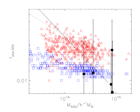
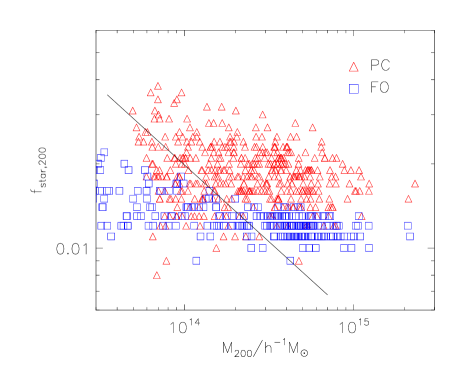
Before dismissing our FO model as unrealistic, however, we note the following:
-
•
As pointed out by Balogh et al. (2008), the GZZ07 data is incompatible with any model that forms galaxies via hierarchical mergers unless there is an unreasonably large star-formation rate in groups at late times.
-
•
The L-Galaxies model produces correlation functions for the galaxy distribution that are consistent with observations with no evidence for a suppression at small separations (Kitzbichler & White, 2008). It is difficult to reconcile this with the need to greatly increase the stellar fraction in groups.
The other simulations mentioned above also predict a slow variation of stellar fraction with mass, although they mostly have stellar fractions that are higher than ours, agreeing with the observations on group scales but having stellar fractions that are too high on cluster scales. For example, the clusters of Ettori et al. (2006) have a stellar fraction of about 0.05 within . The equivalent fraction for massive clusters ( keV) in our own runs is 0.02 for PC and 0.013 for FO. 111Ettori et al. (2006) choose to give stellar fractions in terms of the mean baryon fraction, . The stellar fractions quoted in their paper are thus a factor of 5.6 larger than those listed here.
We conclude that, although the observations are not yet sufficiently robust, stellar mass fractions provide an important test of, and discriminant between, different galaxy formation models.
3.2.5 Scatter in the scaling relations
In this section we investigate why some clusters have slightly more hot gas, and others slightly less, than other clusters of the same mass. Our purpose in doing this is two-fold: firstly to understand the physical reason for this scatter, and secondly to suggest corrections that can be applied to the observations to better allow gas fraction to be used as a probe of cosmology.
First note that, as is evident from Figure 3, the mean gas fractions in the GO run are independent of mass. However, there is scatter about the mean gas fraction that we might hope to relate somehow to the physical properties of the cluster.
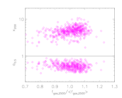
We have checked for correlations of the scatter with every conceivable physical quantity (including substructure, merging history, angular momentum, etc.) and find many weak correlations, but no strong one. Figure 10 shows a positive correlation with concentration, i.e. more concentrated clusters have a greater gas fraction than the average within . Likewise, clusters that form earlier have a greater gas fraction than those that form later. The correlation coefficients for these two relations are 0.29 and , respectively. These may be two aspects of the same relation as concentration shows a negative correlation with formation time. The appendix describes how we measure each of these for the clusters in our simulation. Both are correlated with cluster mass, but it turns out that they are more strongly correlated with each other.
The physical mechanism that may drive the correlations seen in Figure 10 is unclear: it primarily affects the core of the cluster as the correlations get weaker if one measures the gas fraction within larger radii. It may be that the degree of gravitational pre-heating is greater in systems that form later (see, e.g., Mo et al., 2005).
Other quantities that we have tested include the halo angular momentum, merger history and substructure. Once the primary correlation of gas fraction with mass is removed, none of these show any correlation with the residual gas fraction.
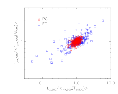
Observationally, of course, an excess core gas fraction is associated with an increase in X-ray luminosity. Thus, as shown in Figure 11, the excess luminosity of a cluster above the mean - relation is correlated with the presence of excess gas in the cluster. The correlation coefficients in this case are 0.51 and 0.73 for the PC and for the FO run, respectively. A similar result was found for the PC run by Stanek et al. (2010). This correlation may serve to reduce the scatter from the major outliers in the gas fraction-mass relation.
3.3 Evolution
3.3.1 Profiles
Figure 12 shows the evolution of the cumulative gas fraction profiles of the 10 most massive clusters, for each of the runs.
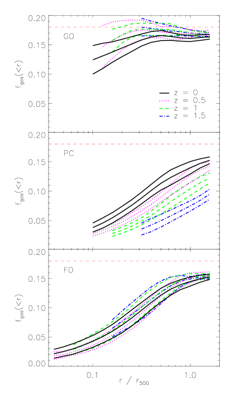
Looking first at the GO run in the upper plot, it can be seen that the gas fraction within remains largely constant over time: this is to be expected for self-similar evolution. As the effective resolution increases (i.e. the ratio of the smoothing length to decreases) so the gas fraction within the cluster core can be seen to be depleted, though still much higher than in the other two runs.
In the PC simulation, the gas fractions at high redshift are much reduced over their current-day values. This is because a large amount of energy has been injected into the ICM at early times, expelling gas from the clusters. Subsequently, the gas falls back into the clusters as the Universe evolves and tends towards (but falls far short of) self-similar evolution. In other words, the early entropy injection becomes relatively less important in more massive systems at late times.
This is in contrast to the behaviour in the FO run. Here we have continual injection of energy so that gas fraction profiles remain constant over time. Although our simulation takes its level of feedback from a semi-analytic model, nevertheless it seems to have achieved a homologous evolution.
Thus, although the PC and FO clusters have indistinguishable gas profiles at the current day, they look very different in the past. This casts doubt on the use of the measured gas fraction as a cosmological probe, but instead opens the possibility that it can be used to determine the nature of the feedback mechanism: in particular to distinguish between early (PC) and continual (FO) heating.
3.3.2 Scaling relations and comparison with observations
Figure 13 shows the hot gas fractions within at a redshift for clusters in our three simulations. For comparison, we also plot high-redshift systems () from a catalogue of clusters observed with Chandra compiled by Maughan et al. (2008). Note that Maughan et al. (2008) do not themselves present values. To compute them, we first determine the total mass, , from the supplied values of (where is defined as the product of the gas mass within and the spectroscopic-like temperature in the spherical annulus ) by using the relation derived from the sample of Vikhlinin et al. (2006). This is the procedure adopted by Maughan et al. (2008, see their Equation 4). The gas fraction then follows upon taking the ratio of the gas mass interior to (tabulated in their paper) to the total mass. The errors on the observational data points in Figure 13 are computed using the supplied statistical errors on the gas mass and the core-excised temperatures. We compute errors on in this way, rather than using the errors on , because the gas mass and temperature are independent measurements.
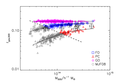
The different evolutionary behaviour of the gas fraction profiles is reflected in that of the mean gas fractions: the PC clusters have significantly smaller gas fractions at early times than those in the FO run. On the whole, the predictions of the FO model provide a closer match to the observational data than those of the PC model, but it seems as if some of the observed data points lie below the lower edge of the FO relation. This could be because the mean cosmic baryon fraction in our simulations is higher than that measured by the WMAP satellite. If we were to repeat our simulations with the measured value of , we would expect all relations in Figure 13 to be shifted downwards, improving the agreement between our FO model and the observations.
However, we note that the observational mass estimates may be lower than the true mass, because they are derived from a relation that was calibrated using clusters with hydrostatic mass estimates. Simulations have shown that the assumption of hydrostatic equilibrium can bias such mass estimates low by (Rasia et al., 2006; Kay et al., 2007b; Nagai et al., 2007; Burns et al., 2008; Piffaretti & Valdarnini, 2008; Meneghetti et al., 2009), because of additional pressure support provided by subsonic bulk motions in the ICM and/or non-thermal components. This would imply a small systematic over-estimate of the gas fraction, so the observational data points in Figure 13 should be shifted downwards and to the right. Another potential source of systematic error is that the masses of high-redshift clusters in the sample of Maughan et al. (2008) were determined by assuming self-similar evolution of the relation.
It is also important to consider the effect of source selection on our results. Observational cluster selection is based on X-ray flux, so may be biased towards systems with higher baryon fractions, particularly at high redshift. It is not possible to quantify this effect precisely using the archival sample of Maughan et al. (2008) since their selection function is unknown. A simple way of estimating the impact of selection effects on our findings is to ask the question: given a typical flux-limited survey, which of our simulated clusters would actually be observed? For illustrative purposes, we choose a flux limit of erg s-1 cm-2, equal to that of the WARPS survey (Horner et al., 2008) from which many of the objects in the Maughan et al. (2008) sample are drawn. The effect of imposing this flux limit at is shown by the dashed line in Figure 13; only objects to the right of this line would be observed by a WARPS-like survey. Note that one of the clusters from Maughan et al. (2008) lies slightly to the left of this line; this is because it is at a lower redshift, . The important point to note is that, for both the PC and FO runs, there is only a narrow mass range where the bias is significant, with most clusters in the two samples remaining unaffected. Even if we took a much higher flux limit, it would require greatly increased scatter about the PC relation for consistency with the observations, which is not intrinsic to the model.
The best-fit parameters to the scaling relation of Equation 3 are shown as a function of redshift in Figure 14. In the case of the GO run, we fit only the mean value of the gas fraction, , which is well-determined. For the other two runs, the shaded regions show the 1-sigma allowed parameter range determined from monte-carlo markov chain fitting. The parameters show considerable scatter, but this scatter is highly correlated. So while it is formally possible for both the PC and FO clusters to have the same value of at , for example, the other parameters must adjust themselves so as to maintain the difference in gas fraction seen in Figure 13.
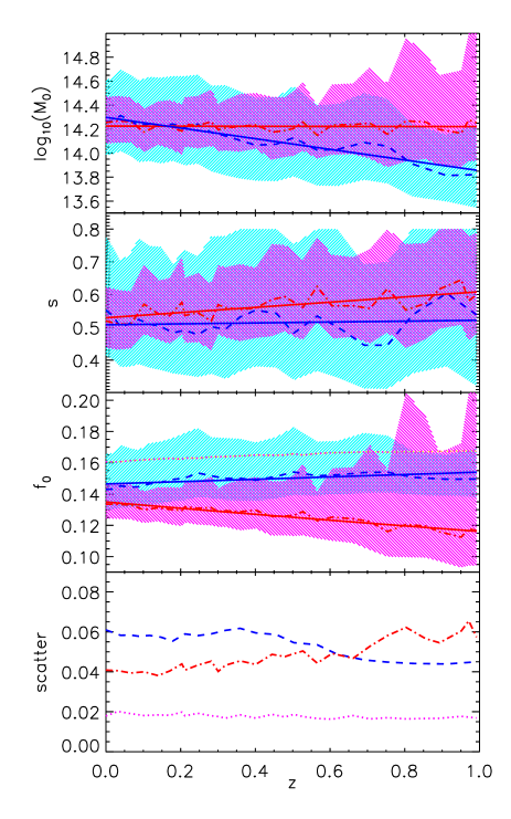
The solid lines in the upper three panels of Figure 14 show straight-line fits to the evolution of each of the parameters with redshift – note that we fit to rather than as it is the former that appears in Equation 3. These fits are listed in Table 3 and are used in the following section when comparing our model predictions with observations.
| Parameter | Model | ||
|---|---|---|---|
| PC | 14.23 | 0.00 | |
| FO | 14.30 | -0.44 | |
| PC | 0.53 | 0.08 | |
| FO | 0.51 | 0.01 | |
| PC | -0.870 | -0.065 | |
| FO | -0.834 | 0.022 |
From the straight-line fits shown in Figure 14, the mean gas fraction within can be predicted for clusters of given mass and redshift using Equation (3). This prediction is compared to observed gas fractions from the sample of Maughan et al. (2008) in Figure 15. What is plotted here is the ratio of the observed gas fraction to the predicted one, so that perfect agreement would correspond to a value of unity, independent of redshift, but with some scatter due to the cluster-to-cluster variation and measurement error. The data are presented in this way since the gas fraction is a function of both cluster mass and redshift. The error bars are computed using the errors on the observed gas fractions (see above for details of how these were determined from the data of Maughan et al. 2008), accounting for the fact that the error on the total mass introduces an extra uncertainty when computing the theoretical prediction for the gas fraction.
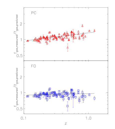
It is immediately apparent that observations favour the FO prediction over the PC one, i.e. limited evolution in gas fraction since . This is shown in Table 4 where we list the allowable parameter ranges for straight line fits to the data both in linear and in – space, where is the ratio of observed to predicted gas fraction within .
| Model | const | slope | scatter |
|---|---|---|---|
| PC linear | 0.074 | ||
| log | 0.028 | ||
| FO linear | 0.071 | ||
| log | 0.034 |
In making these fits, we treat the scatter about the mean relation as an unknown, , independent of mass and redshift. The data are not good enough for a more sophisticated model, and that is likely, anyway, to make little difference to the fit. Given observational data, , and errors, , we estimate the scatter as
| (4) |
where are the best-fit values. We iterate to convergence in , at each stage minimising the chi-squared statistic
| (5) |
Note that the scatter about the best-fit line is, in each case, lower than that seen in the simulations (as shown in the bottom panel of Figure 14). Formally, therefore, neither of the models is a good fit. However, it seems unlikely that the true scatter in will be below that seen in the PC simulation. The uncertainty in the observed values is hard to determine, particularly at high-redshift, so it is quite possible that the size of the error bars has been over-estimated, leading to an under-estimate of the intrinsic scatter.
For the PC simulation, the slope of the observed to simulated gas fraction ratio is incompatible with a horizontal line with high significance. The difference between the best-fit values at and is about 6 times the scatter. Even if we were to account for observational bias in flux-limited samples towards clusters with higher baryon fractions, especially at high redshift, this is simply too large a difference to be explained by selection effects alone (recall our discussion of Figure 13). We conclude that the PC model can be ruled out as a viable cause of entropy generation in the ICM.
The FO simulations, on the other hand, are perfectly consistent with a constant ratio of approximately unity. The slightly lower mean hot gas fraction for the observations as compared to the simulations can be explained by the fact that the latter have a higher mean baryon fraction than the WMAP 7-year value.5
We note that the analysis of Ettori et al. (2009) has many clusters in common with Maughan et al. (2008), but lists total masses and gas fractions that are often in disagreement. We are not certain why this is but note that there are differences in the analysis of the data, particularly in the cluster outskirts. We have repeated the analysis described in this section with the data of Ettori et al. (2009) but the data are much less constraining, principally because they quote much larger error bars. Nevertheless, one should bear in mind that systematic errors in the assumptions made in the data analysis could be degenerate with differences in the simulated ICM physics.
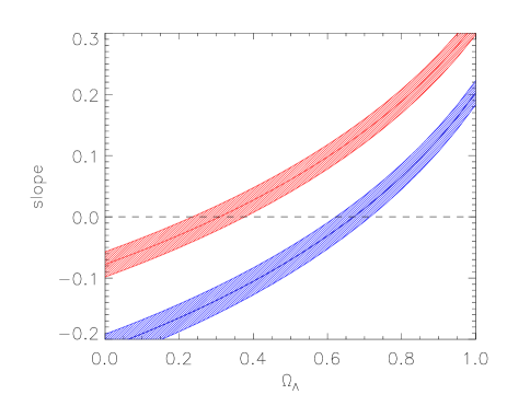
Looking at the problem in reverse, one could ask what errors could be introduced into the determination of cosmological parameters by the choice of an incorrect physical model for the evolution of the ICM. It is not possible to make a precise prediction for this using the current simulations as we only have access to a single realisation with a particular set of cosmological parameters. Nevertheless, fixing the simulated clusters to be the same, Figure 16 shows the effect of changing the observed cluster gas fractions in response to different values of (fixing ). From this, it can be seen that using an incorrect physical model can have a dramatic effect, larger than that induced by changing cosmological parameters within any reasonable range.
The analysis described in this section is necessarily very naive. A full treatment would require a detailed understanding of the selection function of observed clusters, modelling of the scatter in the scaling relations as a function of redshift, and of the mean relations as a function of cosmological parameters. Nevertheless, none of this is likely to alter the basic conclusion that both observed clusters and those derived from our FO model show little evolution in hot gas fractions within out to , whereas the PC model predicts a strong decline.
4 Conclusions
In this paper, we investigate the baryon content of clusters of galaxies in simulations using a variety of physical models for the intracluster medium:
-
•
GO – gravitational heating only with no radiative cooling. The purpose of this model is to test which aspects of the simulation evolve in a self-similar way and to provide a comparison for the other two runs.
-
•
PC - universal preheating to 200 keV cm2 at , plus radiative cooling and star formation. This represents widespread and early heating by objects that lie below the resolution limit of the simulation.
-
•
FO - feedback taken from a semi-analytic model, including heating from both supernovae and active galactic nuclei, but without radiative cooling. The motivation for this model is to test heating from a realistic galaxy population that matches both the luminosity function and the black hole mass function of the current-day Universe.
The differential hot gas fraction profiles of clusters in the GO simulation are approximately constant at radii greater than 0.2 , lying at 90 per cent of the cosmic mean. In the other two simulations, the profiles rise steeply from a low value in the cluster core before bending over to an approximately constant value at large radii: for the most massive clusters, keV, this occurs well within .
The cumulative hot gas fraction profiles of our clusters in both the PC and FO runs lie well below those of the regular, cool-core (CC) clusters observed by Vikhlinin et al. (2006) and Allen et al. (2008). However, they provide a fair match to the non-cool-core (NCC) clusters found in the REXCESS representative cluster survey (Pratt et al., 2010).
When we look at integrated gas fractions within fixed radii, the agreement with observations is mixed. The total gas fraction within shows a stronger variation with cluster mass in the simulations than is seen in the observations. On the other hand, the agreement within is much better, at least on scales above . There is a small offset but that can be explained by the fact that we adopt a mean baryon fraction in our simulations that is higher than the current best-fit value from WMAP, respectively 0.18 and 0.168.
A more slowly-varying function of mass is provided by the differential gas fraction between and . Unfortunately, the scatter in the observational data is currently too large to allow any meaningful comparison with the simulations.
In agreement with previous work, our simulated clusters show a much smaller dependence of stellar fraction on mass than is seen in observations. Our stellar fractions within are about 0.013 for massive clusters, , in the FO run, similar to observed values. The PC run gives slightly higher values, 0.02, whereas previous simulations can have stellar fractions as high as 0.05 (i.e. as much as a third of all the baryons within the cluster turned into stars). On the other hand, for lower-mass clusters, , our mean stellar fractions of 0.015 (FO) and 0.03 (PC) are much lower than the observed value of about 0.05. We note that there is some theoretical difficulty in understanding such a steep dependence of stellar fraction on cluster mass, and that the observational determination of this mass fraction is difficult, especially in low-mass systems. While this should prove a fruitful line of investigation in the future, it is probably too early to draw firm conclusions about the validity of the models.
We have fitted the gas fractions as a function of mass to relations of the form given by Equation 3, with the results shown in Table 1. The scatter about these mean relations is lowest for the GO run and significantly larger for the PC, and especially the FO runs. Unfortunately, the observational data are too poor to provide an accurate measure.
For the GO run, we might expect that the scatter about the mean gas fraction-mass relations has a physical origin in the formation history of the clusters. Indeed, there is a weak correlation/anti-correlation of gas fraction with concentration/formation time (most strongly with the expansion factor at the time that the cluster had accumulated half its current mass). The strongest correlation that might be used observationally to correct for scatter in the gas fractions is that between deviation from the mean - relation and the excess gas fraction.
Although the gas fraction profiles are very similar for both the PC and FO runs at , their evolution is very different. In the former gas is heated and expelled from the clusters at early times, so that the gas is depleted at high redshift and gradually falls back into the cluster over time. By contrast, the continual injection of energy in the FO run leads to evolution that is close to self-similar.
The evolution of halo gas fractions can therefore be used as a strong discriminant between models. We compare our simulated clusters with the compilation of Chandra clusters from Maughan et al. (2008). The observational data are fully-consistent with the FO predictions and disagree with the evolution seen in the PC simulation with high significance. We need to be a little careful in interpreting these results as this is a highly biased sample that may well contain a disproportionate number of luminous clusters at high-redshift. However, the scatter in gas fraction is sufficiently small that, even if we only observed those clusters with high baryon fractions at high redshift, the disagreement between the observations and the PC prediction would still be significant. We conclude that the observations favour continual heating, as in our FO model, over significant preheating at high redshift.
A corollary of the strong dependence of gas fraction evolution on the physics of entropy generation is that it becomes very difficult to use the gas fraction as a probe of cosmology. The differences caused by uncertain gas physics currently swamp those caused by reasonable changes in cosmological parameters. In the future, as both observational data for high-redshift clusters and models of the ICM improve, a joint analysis should be undertaken that considers variations in both cosmological parameters and cluster physics.
The main limitation to our present study is that the absence of cooling in our FO simulation leaves us unable to model CC clusters. Whilst that does not significantly affect the gas fractions when integrated out to , it would be clearly desirable to also reproduce the full range of gas fraction profiles at smaller radii. We are working on ways to introduce cooling into the FO scheme without leading to excess production of cooled gas in CC clusters.
Acknowledgements
This work was supported by the STFC [grant number ST/F002858/1, PhD studentship]
We would like to thank Adrian Jenkins for supplying the
code to generate the initial conditions. The simulations were carried
out using the HPC facility at the University of Nottingham and the
Virgo Consortium facilities at Durham. Analysis was undertaken on the
Archimedes cluster at Sussex. We are grateful to Steve Allen, Stefano
Andreon, Gabriel Pratt, Alistair Sanderson, Alexey Vikhlinin and
especially Ben Maughan for supplying us with observational data and
helping us with its interpretation.
We would like to thank the referee for their constructive
comments which have strengthened this paper.
References
- Allen et al. (2008) Allen S. W., Rapetti D. A., Schmidt R. W., Ebeling H., Morris R. G., Fabian A. C., 2008, MNRAS, 383, 879
- Allen et al. (2004) Allen S. W., Schmidt R. W., Ebeling H., Fabian A. C., van Speybroeck L., 2004, MNRAS, 353, 457
- Allen et al. (2002) Allen S. W., Schmidt R. W., Fabian A. C., 2002, MNRAS, 334, L11
- Andreon (2010) Andreon S., 2010, ArXiv e-prints: 1004.2785
- Arnaud et al. (2007) Arnaud M., Pointecouteau E., Pratt G. W., 2007, A&A, 474, L37
- Ascasibar et al. (2006) Ascasibar Y., Sevilla R., Yepes G., Müller V., Gottlöber S., 2006, MNRAS, 371, 193
- Balogh et al. (2008) Balogh M. L., McCarthy I. G., Bower R. G., Eke V. R., 2008, MNRAS, 385, 1003
- Bernstein et al. (1995) Bernstein G. M., Nichol R. C., Tyson J. A., Ulmer M. P., Wittman D., 1995, AJ, 110, 1507
- Bialek et al. (2001) Bialek J. J., Evrard A. E., Mohr J. J., 2001, ApJ, 555, 597
- Böhringer et al. (2007) Böhringer H., Schuecker P., Pratt G. W., Arnaud M., Ponman T. J., Croston J. H., Borgani S., Bower R. G., Briel U. G., Collins C. A., Donahue M., Forman W. R., Finoguenov A., Geller M. J., Guzzo L., Henry J. P., Kneissl R., Mohr J. J., Matsushita K., Mullis C. R., Ohashi T., Pedersen K., Pierini D., Quintana H., Raychaudhury S., Reiprich T. H., Romer A. K., Rosati P., Sabirli K., Temple R. F., Viana P. T. P., Vikhlinin A., Voit G. M., Zhang Y., 2007, A&A, 469, 363
- Borgani et al. (2005) Borgani S., Finoguenov A., Kay S. T., Ponman T. J., Springel V., Tozzi P., Voit G. M., 2005, MNRAS, 361, 233
- Borgani et al. (2002) Borgani S., Governato F., Wadsley J., Menci N., Tozzi P., Quinn T., Stadel J., Lake G., 2002, MNRAS, 336, 409
- Borgani et al. (2004) Borgani S., Murante G., Springel V., Diaferio A., Dolag K., Moscardini L., Tormen G., Tornatore L., Tozzi P., 2004, MNRAS, 348, 1078
- Brighenti & Mathews (2001) Brighenti F., Mathews W. G., 2001, ApJ, 553, 103
- Burns et al. (2008) Burns J. O., Hallman E. J., Gantner B., Motl P. M., Norman M. L., 2008, ApJ, 675, 1125
- Colless et al. (2001) Colless M., Dalton G., Maddox S., Sutherland W., Norberg P., Cole S., Bland-Hawthorn J., Bridges T., Cannon R., Collins C., Couch W., Cross N., Deeley K., De Propris R., Driver S. P., Efstathiou G., Ellis R. S., Frenk C. S., Glazebrook K., Jackson C., Lahav O., Lewis I., Lumsden S., Madgwick D., Peacock J. A., Peterson B. A., Price I., Seaborne M., Taylor K., 2001, MNRAS, 328, 1039
- Crain et al. (2007) Crain R. A., Eke V. R., Frenk C. S., Jenkins A., McCarthy I. G., Navarro J. F., Pearce F. R., 2007, MNRAS, 377, 41
- Davé et al. (2008) Davé R., Oppenheimer B. D., Sivanandam S., 2008, MNRAS, 391, 110
- De Lucia & Blaizot (2007) De Lucia G., Blaizot J., 2007, MNRAS, 375, 2
- Eisenhardt et al. (2008) Eisenhardt P. R. M., Brodwin M., Gonzalez A. H., Stanford S. A., Stern D., Barmby P., Brown M. J. I., Dawson K., Dey A., Doi M., Galametz A., Jannuzi B. T., Kochanek C. S., Meyers J., Morokuma T., Moustakas L. A., 2008, ApJ, 684, 905
- Eke et al. (1998) Eke V. R., Navarro J. F., Frenk C. S., 1998, ApJ, 503, 569
- Ettori et al. (2006) Ettori S., Dolag K., Borgani S., Murante G., 2006, MNRAS, 365, 1021
- Ettori et al. (2009) Ettori S., Morandi A., Tozzi P., Balestra I., Borgani S., Rosati P., Lovisari L., Terenziani F., 2009, A&A, 501, 61
- Evrard & Henry (1991) Evrard A. E., Henry J. P., 1991, ApJ, 383, 95
- Fabjan et al. (2010) Fabjan D., Borgani S., Tornatore L., Saro A., Murante G., Dolag K., 2010, MNRAS, 401
- Feldmeier et al. (2004) Feldmeier J. J., Mihos J. C., Morrison H. L., Harding P., Kaib N., Dubinski J., 2004, ApJ, 609, 617
- Feldmeier et al. (2002) Feldmeier J. J., Mihos J. C., Morrison H. L., Rodney S. A., Harding P., 2002, ApJ, 575, 779
- Giodini et al. (2009) Giodini S., Pierini D., Finoguenov A., Pratt G. W., Boehringer H., Leauthaud A., Guzzo L., Aussel H., the COSMOS collaboration, 2009, ApJ, 703, 982
- Gonzalez et al. (2005) Gonzalez A. H., Zabludoff A. I., Zaritsky D., 2005, ApJ, 618, 195
- Gonzalez et al. (2000) Gonzalez A. H., Zabludoff A. I., Zaritsky D., Dalcanton J. J., 2000, ApJ, 536, 561
- Gonzalez et al. (2007) Gonzalez A. H., Zaritsky D., Zabludoff A. I., 2007, ApJ, 666, 147
- Horner et al. (2008) Horner D. J., Perlman E. S., Ebeling H., Jones L. R., Scharf C. A., Wegner G., Malkan M., Maughan B., 2008, ApJ Supp., 176, 374
- Kaiser (1991) Kaiser N., 1991, ApJ, 383, 104
- Kay et al. (2007a) Kay S. T., da Silva A. C., Aghanim N., Blanchard A., Liddle A. R., Puget J.-L., Sadat R., Thomas P. A., 2007a, MNRAS, 377, 317
- Kay et al. (2007b) —, 2007b, MNRAS, 377, 317
- Kitzbichler & White (2008) Kitzbichler M. G., White S. D. M., 2008, MNRAS, 391, 1489
- Komatsu et al. (2010) Komatsu E., Smith K. M., Dunkley J., Bennett C. L., Gold B., Hinshaw G., Jarosik N., Larson D., Nolta M. R., Page L., Spergel D. N., Halpern M., Hill R. S., Kogut A., Limon M., Meyer S. S., Odegard N., Tucker G. S., Weiland J. L., Wollack E., Wright E. L., 2010, ArXiv e-prints: 1001.4538
- Kravtsov et al. (2005) Kravtsov A. V., Nagai D., Vikhlinin A. A., 2005, ApJ, 625, 588
- Krick et al. (2006) Krick J. E., Bernstein R. A., Pimbblet K. A., 2006, ApJ, 131, 168
- Laganá et al. (2008) Laganá T. F., Lima Neto G. B., Andrade-Santos F., Cypriano E. S., 2008, A&A, 485, 633
- LaRoque et al. (2006) LaRoque S. J., Bonamente M., Carlstrom J. E., Joy M. K., Nagai D., Reese E. D., Dawson K. S., 2006, ApJ, 652, 917
- Mantz et al. (2009a) Mantz A., Allen S. W., Ebeling H., Rapetti D., Drlica-Wagner A., 2009a, ArXiv e-prints: 0909.3099
- Mantz et al. (2009b) Mantz A., Allen S. W., Rapetti D., Ebeling H., 2009b, ArXiv e-prints: 0909.3098
- Maughan et al. (2008) Maughan B. J., Jones C., Forman W., Van Speybroeck L., 2008, ApJ Supp., 174, 117
- Mazzotta et al. (2004) Mazzotta P., Rasia E., Moscardini L., Tormen G., 2004, MNRAS, 354, 10
- McCarthy et al. (2009) McCarthy I. G., Schaye J., Ponman T. J., Bower R. G., Booth C. M., Dalla Vecchia C., Crain R. A., Springel V., Theuns T., Wiersma R. P. C., 2009, ArXiv e-prints: 0911.2641
- Meneghetti et al. (2009) Meneghetti M., Rasia E., Merten J., Bellagamba F., Ettori S., Mazzotta P., Dolag K., 2009, arXiv: astro-ph/0912.1343
- Mo et al. (2005) Mo H. J., Yang X., van den Bosch F. C., Katz N., 2005, MNRAS, 363, 1155
- Muanwong et al. (2006) Muanwong O., Kay S. T., Thomas P. A., 2006, ApJ, 649, 640
- Muanwong et al. (2002) Muanwong O., Thomas P. A., Kay S. T., Pearce F. R., 2002, MNRAS, 336, 527
- Nagai et al. (2007) Nagai D., Kravtsov A. V., Vikhlinin A., 2007, ApJ, 668, 1
- Navarro et al. (1995) Navarro J. F., Frenk C. S., White S. D. M., 1995, MNRAS, 275, 720
- Navarro et al. (1997) —, 1997, ApJ, 490, 493
- Pearce et al. (1994) Pearce F. R., Thomas P. A., Couchman H. M. P., 1994, MNRAS, 268, 953
- Piffaretti & Valdarnini (2008) Piffaretti R., Valdarnini R., 2008, A&A, 491, 71
- Ponman et al. (2003) Ponman T. J., Sanderson A. J. R., Finoguenov A., 2003, MNRAS, 343, 331
- Pratt et al. (2010) Pratt G. W., Arnaud M., Piffaretti R., Böhringer H., Ponman T. J., Croston J. H., Voit G. M., Borgani S., Bower R. G., 2010, A&A, 511, A85+
- Pratt et al. (2006) Pratt G. W., Arnaud M., Pointecouteau E., 2006, A&A, 446, 429
- Puchwein et al. (2010) Puchwein E., Springel V., Sijacki D., Dolag K., 2010, ArXiv e-prints: 1001.3018
- Rasia et al. (2006) Rasia E., Ettori S., Moscardini L., Mazzotta P., Borgani S., Dolag K., Tormen G., Cheng L. M., Diaferio A., 2006, MNRAS, 369, 2013
- Sadat et al. (2005) Sadat R., Blanchard A., Vauclair S. C., Lumb D. H., Bartlett J., Romer A. K., Bernard J., Boer M., Marty P., Nevalainen J., Burke D. J., Collins C. A., Nichol R. C., 2005, A&A, 437, 31
- Sanderson et al. (2003) Sanderson A. J. R., Ponman T. J., Finoguenov A., Lloyd-Davies E. J., Markevitch M., 2003, MNRAS, 340, 989
- Short & Thomas (2009) Short C. J., Thomas P. A., 2009, ApJ, 704, 915
- Short et al. (2010) Short C. J., Thomas P. A., Young O. E., Pearce F. R., Jenkins A., Muanwong O., 2010, ArXiv e-prints: 1002.4539
- Spergel et al. (2003) Spergel D. N., Verde L., Peiris H. V., Komatsu E., Nolta M. R., Bennett C. L., Halpern M., Hinshaw G., Jarosik N., Kogut A., Limon M., Meyer S. S., Page L., Tucker G. S., Weiland J. L., Wollack E., Wright E. L., 2003, ApJ Supp., 148, 175
- Springel et al. (2005) Springel V., White S. D. M., Jenkins A., Frenk C. S., Yoshida N., Gao L., Navarro J., Thacker R., Croton D., Helly J., Peacock J. A., Cole S., Thomas P., Couchman H., Evrard A., Colberg J., Pearce F., 2005, Nat., 435, 629
- Stanek et al. (2010) Stanek R., Rasia E., Evrard A. E., Pearce F., Gazzola L., 2010, ApJ, 715, 1508
- Sun et al. (2009) Sun M., Voit G. M., Donahue M., Jones C., Forman W., Vikhlinin A., 2009, ApJ, 693, 1142
- Sutherland & Dopita (1993) Sutherland R. S., Dopita M. A., 1993, ApJ Supp., 88, 253
- Tornatore et al. (2003) Tornatore L., Borgani S., Springel V., Matteucci F., Menci N., Murante G., 2003, MNRAS, 342, 1025
- Tozzi et al. (2003) Tozzi P., Rosati P., Ettori S., Borgani S., Mainieri V., Norman C., 2003, ApJ, 593, 705
- Vikhlinin et al. (2006) Vikhlinin A., Kravtsov A., Forman W., Jones C., Markevitch M., Murray S. S., Van Speybroeck L., 2006, ApJ, 640, 691
- Voit et al. (2005) Voit G. M., Kay S. T., Bryan G. L., 2005, MNRAS, 364, 909
- Weiner et al. (2009) Weiner B. J., Coil A. L., Prochaska J. X., Newman J. A., Cooper M. C., Bundy K., Conselice C. J., Dutton A. A., Faber S. M., Koo D. C., Lotz J. M., Rieke G. H., Rubin K. H. R., 2009, ApJ, 692, 187
- Zibetti et al. (2005) Zibetti S., White S. D. M., Schneider D. P., Brinkmann J., 2005, MNRAS, 358, 949
Appendix
The central concentration of clusters can be determined by measuring the mass at two different over-densities, for example and . Together, these uniquely determine the parameters of the NFW profile (Navarro et al., 1997) without any need to fit the profile as a function of radius.222We provide IDL routines to do this at http://astronomy.susx.ac.uk/petert/nfw.pro. To test the effectiveness of this procedure, we show in Figure 17 the value of predicted by the NFW fit (i.e. the NFW scale radius, , times the concentration, ) versus the actual value. As can be seen, the two agree very well, confirming that the clusters are well-fit by the NFW profile out to this radius.

Cluster concentrations are often thought to have a dependence upon cluster mass, with more massive clusters having lower concentrations. That is indeed the case, but we find a much stronger correlation with cluster formation time, as illustrated in Figure 18. Here the formation time is taken to be the value of the expansion factor when the total mass of all the subhalos that will go on to make up the cluster equal one fifth of the final cluster mass, but other definitions give similar correlations. We plot expansion factor rather than age as this gives a more linear correlation. The results are shown here for the GO simulation; those for the PC and FO runs are very slightly different because of the contribution of the baryons to the total mass.
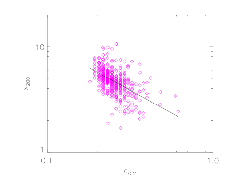
On removing the best-fitting correlation (shown as a solid line in the figure), the residual concentration shows no dependence on mass. The correlation with mass is thus a secondary one that follows because low mass clusters tend to form at lower expansion factors than more massive ones.