Thick brane solutions and topology change transition on black hole backgrounds

Abstract

We consider static, axisymmetric, thick brane solutions on higher dimensional, spherically symmetric black hole backgrounds. It was found recently CF (1), that in cases when the thick brane has more than 2 spacelike dimensions, perturbative approaches break down around the corresponding thin solutions for Minkowski type topologies. This behavior is a consequence of the fact that thin solutions are not smooth at the axis, and for a general discussion of possible phase transitions in the system, one needs to use a non-perturbative approach. In the present paper we provide an exact, numerical solution of the problem both for black hole- and Minkowski type topologies with arbitrary number of brane and bulk dimensions. We also illustrate a topology change transition in the system for a 5-dimensional brane embedded in a 6-dimensional bulk.

I Introduction

Curvature corrections to Dirac-Nambu-Goto (DNG) membranes Dirac (2, 3, 4) in higher dimensional black hole backgrounds attracts a lot of attention recently in several different areas of modern physics. The simplest corrections to the DNG brane action originate from small thickness perturbations that are quadratic at the leading order in the thickness of the brane Carter2 (5). These type of corrections have been studied lately in the case of a static, axisymmetric brane on the background of a spherically symmetric black hole in arbitrary number of dimensions CF (1, 6).

This, so called, brane - black hole (BBH) system, in the infinitely thin case, was first introduced by Frolov Frolov (7) as a toy model for the study of merger- and topology changing transitions between higher dimensional black type solutions (or phases) of the Einstein field equations Kol1 (8, 9, 10). The model also turned out to be very useful through the AdS/CFT correspondence for the study of phase transitions in certain strongly coupled gauge theories MMT1 (11, 12), while the higher dimensional generalizations of the Bernstein conjecture B1 (13, 14), the study of the stability of brane - black hole systems B3 (15), and the question of possible micro black hole formations in high energy collisions (like of the LHC) flactan (18) are also important directions which are dealing with similar setup, and provide motivation for the study of the curvature corrected problem.

Stiffness (or thickness) corrections to the BBH system has been studied first in FG (6), with a perturbative approach near the critical solution of the thin system in the Rindler zone. It was found that when the brane has more than 2 spatial dimensions, supercritical solutions behave quite differently from subcritical ones, and no evidence for the existence of such solutions has been found. A possible explanation of this behavior was that stiffness corrections to the brane action break the symmetry between the super- and subcritical solutions, and quantum-gravitational effects might cure the problem.

The thickness corrected BBH system has been further studied in CF (1) within a more general perturbative approach that also looked away from the Rindler zone. In accordance with FG (6), it was found that no regular subcritical thick solutions exist if the brane has more than 2 spacelike dimensions. This result however obtained a simple explanation with observing the fact that perturbative approaches break down around the corresponding thin solutions at the axis of the system, because the zero order (thin) solutions are not smooth there. As a consequence, the topology change transition in the thick system can not be studied in the general case within a perturbative approach, and one needs to find a new, exact solution of the problem for Minkowski type topologies.

In the present paper we provide an exact numerical solution of the thick-BBH problem with arbitrary number of brane and bulk dimensions for both Minkowski- and black hole topologies. This work is an organic continuation of our previous perturbative approach and we kindly refer the reader to CF (1) for those definitions, notation and results that might be missing here and would make the present paper completely self-contained.

The plan of the paper is as follows. In Sec. II we run trough the same quick overview of the infinitely thin case that we provided in CF (1), and reintroduce the most important parts of the BBH setup to make the paper self-contained. In Sec. III we write up the curvature corrected DNG action and introduce the correction parameters. In Sec. IV we derive the Euler-Lagrange equation and the equation of motion for the thick BBH system. In Sec. V the regularity conditions are discussed while in Sec. VI the far distance asymptotic solution is obtained. In Sec. VII we provide the exact, numerical solution of the problem in the near horizon region for both topologies, and in Sec. VIII a topology change transition is analyzed by considering the energy properties of a quasi-static thick brane evolution in the case of a 5-dimensional brane in a 6-dimensional bulk.

II The thin BBH system setup

Let us overview, in this section, the important properties of the BBH system, introduced in Frolov (7), that we intend to study in the presence of a small brane thickness in the following sections. We consider static brane configurations in the background of a static, spherically symmetric bulk black hole. The metric of an $N$-dimensional, spherically symmetric black hole spacetime is

$$ds^{2}=g_{ab}dx^{a}dx^{b}=-fdt^{2}+f^{-1}dr^{2}+r^{2}d\Omega_{N-2}^{2}\ ,$$ (1)

where $f=f(r)$ and $d\Omega_{N-2}^{2}$ is the metric of an $N-2$ dimensional unit sphere. One can define coordinates $\theta_{i}(i=1,\dots,N-2)$ on this sphere with the relation

$$d\Omega_{i+1}^{2}=d\theta_{i+1}^{2}+\sin^{2}\theta_{i+1}d\Omega_{i}^{2}\ .$$ (2)

The explicit form of $f$ is not important, it is only assumed that $f$ is zero at the horizon $r_{0}$, and it grows monotonically to $1$ at the spatial infinity $r\rightarrow\infty$, where it has the asymptotic form Tangherlini (19),

$$f=1-\left(\frac{r_{0}}{r}\right)^{N-3}\ .$$ (3)

In the zero thickness case, the test brane configurations, in an external gravitational field, can be obtained by solving the equation of motion coming from the Dirac-Nambu-Goto action Dirac (2, 3, 4),

$$S=\int d^{D}\zeta\sqrt{-\mbox{det}\gamma_{\mu\nu}}\ ,$$ (4)

where $\gamma_{\mu\nu}$ is the induced metric on the brane

$$\gamma_{\mu\nu}=g_{ab}\frac{\partial x^{a}}{\partial\zeta^{\mu}}\frac{\partial x^{b}}{\partial\zeta^{\nu}}\ ,$$ (5)

and $\zeta^{\mu}(\mu=0,\dots,D-1)$ are coordinates on the brane world sheet. The brane tension does not enter into the brane equations, thus for simplicity it can be put equal to $1$. It is also assumed that the brane is static and spherically symmetric, and its surface is chosen to obey the equations

$$\theta_{D}=\dots=\theta_{N-2}=\pi/2\ .$$ (6)

With the above symmetry properties the brane world sheet can be defined by the function $\theta_{D-1}=\theta(r)$ and we shall use coordinates $\zeta^{\mu}$ on the brane as

$$\zeta^{\mu}=\{t,r,\phi_{1},\dots,\phi_{n}\}\quad\mbox{with}\quad n=D-2\ .$$ (7)

With this parametrization the induced metric on the brane is

$$\gamma_{\mu\nu}d\zeta^{\mu}d\zeta^{\nu}=-fdt^{2}+\left[\frac{1}{f}+r^{2}{\dot{\theta}}^{2}\right]dr^{2}+r^{2}\sin^{2}\theta d\Omega_{n}^{2},$$ (8)

where, and throughout this paper, a dot denotes the derivative with respect to $r$, and the action (4) reduces to

$$S = \Delta t\mathcal{A}_{n}\int\mathcal{L}_{0}\ dr\ ,$$ (9)

$$\mathcal{L}_{0} = r^{n}\sin^{n}\theta\sqrt{1+fr^{2}{\dot{\theta}}^{2}}\ ,$$ (10)

where $\Delta t$ is the interval of time and $\mathcal{A}_{n}=2\pi^{n/2}/\Gamma(n/2)$ is the surface area of a unit $n$-dimensional sphere.

III The thick brane action

In the case of a thick brane, the curvature corrected effective brane action is obtained by Carter and Gregory Carter2 (5), and the corrections to the thin DNG action are induced by small thickness perturbations

$$S=\int d^{D}\zeta\sqrt{-\mbox{det}\gamma_{\mu\nu}}\left[-\tfrac{8\mu^{2}}{3\ell}(1+C_{1}R+C_{2}K^{2})\right],$$ (11)

where $R$ is the Ricci scalar, $K$ is the extrinsic curvature scalar of the brane and the coefficients $C_{1}$ and $C_{2}$ are expressed by the wall thickness parameter $\ell$ as

$$C_{1}=\frac{\pi^{2}-6}{24}\ell^{2}\ ,\qquad C_{2}=-\frac{1}{3}\ell^{2}.$$ (12)

The parameter $\mu$ is related to the thickness by

$$\ell=\frac{1}{\mu\sqrt{2\lambda}}$$ (13)

which originates from a field theoretical domain-wall model, where $\mu$ is the mass parameter and $\lambda$ is the coupling constant of the scalar field.

After integrating out the spherical symmetric part and the time dependence on the introduced static, spherically symmetric, higher dimensional black hole background, one obtains (see also CF (1))

$$S = \Delta t\mathcal{A}_{n}\int\mathcal{L}\ dr\ ,$$ (14)

$$\mathcal{L} = -\frac{8\mu^{2}}{3\ell}\mathcal{L}_{0}[1+\varepsilon\delta]\ ,$$ (15)

where we introduced the notations

$$\varepsilon=\frac{\ell^{2}}{L^{2}},\qquad\delta = aK^{2}+bQ\ ,$$ (16)

with

$$Q=K^{a}_{b}K^{b}_{a},\quad a=\frac{\pi^{2}-14}{24}L^{2},\quad b=\frac{6-\pi^{2}}{24}L^{2}\ ,$$ (17)

and $L$ is the relevant dynamical length scale of the system which has to be large compared to the thickness parameter $\ell$. The explicit expressions of the curvature scalars $K$ and $Q$ are given in (35) and (36) of CF (1).

IV The Euler-Lagrange equation

The curvature corrected DNG-brane action has a dependence on the second derivative of $\theta$, thus the Euler-Lagrange equation of the problem reads

$$\frac{d^{2}}{dr^{2}}\left(\frac{\partial\mathcal{L}}{\partial\ddot{\theta}}\right)-\frac{d}{dr}\left(\frac{\partial\mathcal{L}}{\partial\dot{\theta}}\right)+\frac{\partial\mathcal{L}}{\partial\theta}=0\ .$$ (18)

Plugging the thickness corrected Lagrangian density (15) into (18) we get

$$\!\!\!\!\!\!\!\!\!\!\!\!\!\!\!\!\!\!\!\!0 = \frac{d}{dr}\left(\frac{\partial\mathcal{L}_{0}}{\partial\dot{\theta}}\right)-\frac{\partial\mathcal{L}_{0}}{\partial\theta}$$ (19)

$$- \varepsilon\left[\frac{d^{2}}{dr^{2}}\left(\frac{\partial(\mathcal{L}_{0}\delta)}{\partial\ddot{\theta}}\right)-\frac{d}{dr}\left(\frac{\partial(\mathcal{L}_{0}\delta)}{\partial\dot{\theta}}\right)+\frac{\partial(\mathcal{L}_{0}\delta)}{\partial\theta}\right],$$

from which the actual equation of motion becomes

$$\theta^{(4)} + T_{1}\theta^{(3)}+T_{2}(\ddot{\theta},\dot{\theta},\theta,f^{(3)},\ddot{f},\dot{f},f,r)=0\ ,$$ (20)

where

$$T_{1} = \frac{1}{rfF^{2}}\left[\right.(2n+4)f+4r\dot{f}+2nrf\cot\theta\dot{\theta}$$ (21)

$$+ r^{2}f\left[2(n-3)f-r\dot{f}\right]\dot{\theta}^{2}$$

$$+ 2nr^{3}f^{2}\cot\theta\dot{\theta}^{3}-10r^{3}f^{2}\ddot{\theta}\left.\right]\ ,$$

and $T_{2}$ is given in the appendix.

The goal of this paper is to provide a regular, exact, numerical solution of (20) in arbitrary brane and bulk dimensions for both Minkowski- and black hole type topologies, and study the properties of a quasi-static brane transition between the two type of solutions.

V Regularity conditions

V.1 Minkowski embedding case

As a first step we consider the asymptotic behavior of (20) near the axis of the system ($\theta=0$) in the Minkowski embedding case, where the perturbative approaches failed to provide regular solutions in the dimensions $n\geq 2$. The asymptotic equation (obtained by taking the series expansion of (20) around $\theta=0$) reads

$$\frac{s_{3}}{\theta^{3}}+\frac{s_{2}}{\theta^{2}}+\frac{s_{1}}{\theta}+s_{0}+\dots=0\ ,$$ (22)

where the functions $s_{1}$, $s_{2}$, and $s_{3}$ are given in the appendix. For a regular solution one needs to require $s_{3}$, $s_{2}$ and $s_{1}$ to disappear at $r_{1}$.

The requirement $s_{3}|_{r_{1}}=0$ is automatically satisfied in the cases of $n=0$ and $n=2$. For other dimensions we obtain the formula

$$\dot{\theta}|_{r_{1}}=\pm\left.\sqrt{\frac{-(b+an)}{2(2a+b-an)r^{2}f}}\right|_{r_{1}}\ .$$ (23)

We are looking for real solutions, hence we have the condition

$$\frac{-(b+an)}{2(2a+b-an)}\geq 0\ .$$ (24)

Plugging the explicit values of $a$ and $b$ into (24) one can find that the inequality is satisfied for all $n\geq 3$. In the case of $n=1$, the regularity condition (23) has no real solution for $\dot{\theta}|_{r_{1}}$, which is a rather unexpected result. Note that this result is independent of the explicit values of $a$ and $b$.

From the requirements $s_{2}|_{r_{1}}=0$ and $s_{1}|_{r_{1}}=0$ we obtain unique conditions for $\ddot{\theta}|_{r_{1}}=g(\dot{\theta}|_{r_{1}})$ and $\theta^{(3)}|_{r_{1}}=h(\dot{\theta}|_{r_{1}},\ddot{\theta}|_{r_{1}})$, where the functions $g$ and $h$ are given in the appendix.

Accordingly, one can always find a regular solution for the equation (20) at the axes ($\theta|_{r_{1}}=0$) if $n\geq 3$. In this case the initial conditions are also uniquely fixed by the regularity conditions. In the cases of $n=0$ and $n=2$, regular solutions do exist, however one has a freedom in fixing the initial condition $\dot{\theta}|_{r_{1}}$. Having fixed $\dot{\theta}|_{r_{1}}$, the remaining conditions are uniquely determined.

In the $n=1$ case, the regularity requirements can not be satisfied with the presented method. It is interesting however, that in this case the perturbative approach worked well, and provided unique, regular solution to the problem. Furthermore, as explicitly constructed field theoretical domain-wall models Fl1 (16, 17) clearly show the existence of regular solutions in this case, we believe that the obtained irregularity has no any physical meaning, rather it originates from some kind of break down of the applied method in the special case of $n=1$. A similar problem occurred for example during the integration of the far distance solution in CF (1), where in the $n=3$ case, the solution developed a resonant term. Unfortunately, since the equation of motion in the present exact case is so complicated and so highly non-linear, it is very difficult to follow up analytically the source of this irregular behavior, and thus its origin is presently not clear to the author.

V.2 Black hole embedding case

In the black hole embedding case the perturbative approach provided regular thick solutions in every brane dimensions. Nevertheless, for a complete analysis, we examine the asymptotic behavior of (20) near the black hole horizon and compute the exact, numerical solution of the problem.

As $r\rightarrow r_{0}$, (i.e. on the horizon), the metric function $f(r)$ goes to zero (see (3)) but all of its derivatives are nonzero and finite. We can thus consider the asymptotic behavior of (20) by taking its series expansion around $f(r)=0$, and get

$$\frac{y_{2}}{f^{2}}+\frac{y_{1}}{f}+y_{0}+\dots=0\ ,$$ (25)

where $y_{1}$ and $y_{2}$ are given in the appendix. Similarly to the Minkowski embedding case, from $y_{2}$ one can obtain a unique condition for $\ddot{\theta}|_{r_{0}}=G(\dot{\theta}|_{r_{0}})$, and another for $\theta^{(3)}|_{r_{0}}=H(\dot{\theta}|_{r_{0}},\ddot{\theta}|_{r_{0}})$ from $y_{1}$. The functions $G$ and $H$ are given in the appendix. In addition one can fix $\theta|_{r_{0}}$ arbitrarily between $0$ and $\pi/2$ (which we will actually do later to consider a quasi-static brane evolution), however one still remains free to fix the initial condition $\dot{\theta}|_{r_{0}}$.

Accordingly, the black hole embedding problem can be regularly solved in any dimension, but the regularity requirements do not fix the initial conditions uniquely. For being able to provide an exact, numerical solution, we will adopt the initial condition for $\dot{\theta}|_{r_{0}}$ from the perturbative approach CF (1), where it was uniquely fixed by regularity considerations. This choice is supported by the fact that in the black hole embedding case there is no problem with the perturbative approach around the thin solution, and the exact thick solution is dominated by the linear term in the $\varepsilon$-expansion on the horizon. The contributions of the higher order terms to the $\dot{\theta}|_{r_{0}}$ initial condition are negligible.

VI The far distance solution

As $r\rightarrow\infty$ the far distance solution can be obtained from the condition that the brane behaves asymptotically as a $D-1$-dimensional plane. We look for the solution in the form

$$\theta=\frac{\pi}{2}+\nu(r),$$ (26)

where $\nu(r)$ is small and we keep only its linear terms in (20). The asymptotic equation reads

$$\nu^{(4)}+\tfrac{2(n+2)}{r}\nu^{(3)}-k\ddot{\nu}-\tfrac{k(n+2)}{r}\dot{\nu}-\tfrac{nk}{r^{2}}\nu=0\ ,$$ (27)

where $k=(8(a+b)\varepsilon)^{-1}$.

It is instructive to compare (27) to the asymptotic form of the perturbation equation (57) of CF (1). As one would expect, the terms up to the second derivative are identical, while the $3rd$- and $4th$-order terms in (27) are the explicit correspondents of the source term that appears in (57) of CF (1).

For the solution, we obviously expect the same behavior that we obtained in the perturbative approach, although (27) can not be integrated in a simple closed form. In order to check our expectation, we map analytically the point at infinity into the origin using the inversion transformation method (see eg. BO (21))

$$r = \frac{1}{t}\ ,$$

$$\frac{d}{dr} = -t^{2}\frac{d}{dt}\ ,$$

$$\frac{d^{2}}{dr^{2}} = t^{4}\frac{d^{2}}{dt^{2}}+2t^{3}\frac{d}{dt}\ ,$$

and so on, and look for the solution of the transformed asymptotic equation

$$\nu^{(4)}+\tfrac{2(4-n)}{t}\nu^{(3)}-\tfrac{k}{t^{4}}\nu^{\prime\prime}+\tfrac{nk}{t^{5}}\nu^{\prime}-\tfrac{nk}{t^{6}}\nu=0$$ (28)

as $t\rightarrow 0$. In (28) a prime denotes a derivative with respect to $t$.

Even though we observe that (28) has an irregular singular point at $t=0$, one can easily find a completely regular, exact solution

$$\nu(t)=Pt\quad\Longrightarrow\quad\nu(r)=\frac{P}{r}+\dots\ .$$ (29)

This is exactly the far distance behavior that we expected, and the coefficient $P$, just as in the thin case, can be referred as the distance of the brane from the equatorial plane at infinity.

VII Numerical solution in the near horizon region

After obtaining the regularity conditions and providing the far distance solution of the exact curvature corrected problem, we consider the numerical solution of (20) in the near horizon region. Since we found that the initial conditions are not completely fixed for Minkowski embedding topologies in the cases of $n=0$ and $2$, and also concluded that one can not satisfy the regularity condition (24) in the $n=1$ (sheet) case with the presented method, we choose to illustrate the numerical solution in the case of a $D=5$-dimensional ($n=3$) thick brane embedded in a 6-dimensional bulk.

Within the perturbative description (see CF (1) for details) we could not approach the curvature singularity arbitrary close unless we adjusted the thickness of the brane accordingly by changing the value of the perturbation parameter $\varepsilon$ in every step. Instead, the method we followed was fixing $\varepsilon$ to its maximum value, which is equivalent to choose the thickest possible brane configuration for a previously obtained length scale parameter $L$ that had been determined by the boundary position ($\theta_{0}$ or $r_{1}$) of the brane. As we approached the singularity, the absolute maximum of the perturbations were growing and finally we arrived to a minimal $\theta_{0}$ value, at which the applied perturbation method reached its limitation.

With the present, exact solution however, nothing prevents us to approach the singularity as close as we please, and the only restriction we have to bear in mind is the validity of the curvature corrected DNG-brane action (11), i.e.

$$\frac{\ell}{L}\ll 1\ .$$

By keeping the concept of obtaining the thickest possible brane configuration for given boundary data, just as in the perturbative approach, we choose to fix the perturbation parameter $\varepsilon$ to its maximum value obtained from the condition

$$\left.\frac{\ell}{L}\right|_{max}\sim 0.1\quad\Longrightarrow\quad\varepsilon_{max}\equiv\left.\frac{\ell^{2}}{L^{2}}\right|_{max}\simeq 0.01\ .$$

This requirement provides us the thickest possible brane configurations for every given length scale determined by the boundary data $\theta_{0}$ with no restriction on how close we are to the curvature singularity.

VII.1 Minkowski embedding solutions

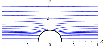
In the perturbative approach, regular thick brane solutions did not exist for Minkowski topologies if the brane had more than two spacelike dimensions, i.e. for $n\geq 2$. In Fig. 1, we have plotted a set of exact thick brane solutions with varying boundary condition ($\theta_{0}$ for black hole embeddings and $r_{1}$ for Minkowski embeddings) in the case of a 5-dimensional ($n=3$) brane embedded in a 6-dimensional bulk.

Figure 1: The picture shows a sequence of subcritical and supercritical thick brane solutions in the case when a $D=5$ dimensional brane embedded into a $N=6$ dimensional bulk. The different configurations belong to different initial conditions of $r_{1}$ and $\theta_{0}$, respectively. For simplicity, the bulk black hole’s horizon radius is put to be 1, and $R$ and $Z$ are the standard cylindrical coordinates.

There is no apparent difference on Fig. 1 if we compare it to the corresponding thin solutions. This is simply because we are considering second order curvature corrections to the thin brane action so the effects are indeed very tiny. To make these effects visible we plot a sequence of the difference function

$$\Delta\theta(r)=\theta(r)-\theta_{DNG}(r),$$

of the corresponding thick and thin exact solutions, which is the analog of the perturbation function $\varphi(r)$ defined in (41) of CF (1).

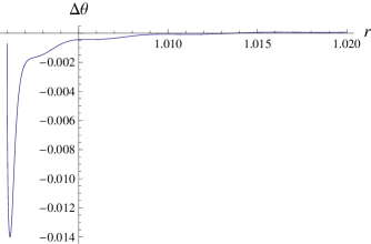
The qualitative behavior of the individual $\Delta\theta$ curves are very similar to the $\varphi$ perturbations that we obtained in the $n=1$ case in CF (1). The curves that are very close to the horizon has a sharp negative maximum and change sign before decaying. On the actual shape of the curves however we can observe the effect of the higher orders as having an extra oscillatory pattern. In Fig. 2 we have plotted a $\Delta\theta$ curve corresponding to $r_{1}=1.001$ boundary condition.

Figure 2: The picture shows a near horizon $\Delta\theta$ curve with minimum horizon distance $r_{1}=1.001$.

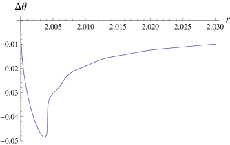
If we go away from the horizon, the difference function becomes more spread and doesn’t change sign before decaying. The negative maximum and the oscillatory extra pattern are still present. In Fig. 3 we have plotted a $\Delta\theta$ curve corresponding to $r_{1}=2$ boundary condition.

Figure 3: The picture shows a $\Delta\theta$ curve a bit further away from the black hole horizon with minimum horizon distance $r_{1}=2$.

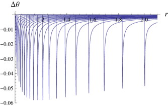
As we can see, there is no essential difference in the individual $\Delta\theta$ curves compared to the perturbation function $\varphi$ obtained in CF (1) in the $n=1$ case. A remarkable difference appears however, if we take a look on the absolute maximum of the curves as we increase the minimum distance parameter $r_{1}$. In Fig. 4 we have plotted a sequence of $\Delta\theta$ curves.

Figure 4: The picture shows a sequence of $\Delta\theta$ curves with increasing minimum distance parameter in the $1.001\leq r_{1}\leq 2$ interval.

It can be seen that the absolute maximum of the difference function curves does not decay monotonically with increasing distance from the horizon. Instead, it has a growing tendency until it reaches a maximum around $r_{1}\simeq 1.15$, after which it starts decaying monotonically as one would expect. The concrete numerical values of the absolute maximum of the curves are not relevant as they depend on the chosen normalization condition, i.e. on the maximum length parameter $L$. In analyzing the Minkowski embedding solutions, we have used the normalization parameter that belongs to the boundary condition $\theta_{0}=\tfrac{\pi}{18}$.

Apart, of course, from the very existence of the thick solutions in the $n\geq 2$ cases, the above non-monotonic decaying is an interesting and clear difference between the exact and perturbative solutions.

VII.2 Black hole embedding solutions

The non-monotonicity in the maximum values of the difference function $\Delta\theta$ with respect to the initial value parameter $\theta_{0}\in(0,\tfrac{\pi}{2}]$ is also present in the black hole embedding case. As we mentioned earlier, the regularity requirements do not fix the $\dot{\theta}|_{r_{0}}$ conditions for the black hole case, and to provide a set of exact solutions we took the missing conditions from our previously obtained perturbative results CF (1).

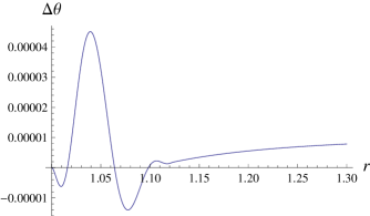
We also discussed that with the presented exact solution we can approach the curvature singularity in principle as close as we please, and it is only the capacity of our computing facility that can put some limitation on us. Taking into account our limits, we have chosen to solve our equation starting from the parameter $\theta_{0}=\tfrac{\pi}{900}$, which is a significant increase compared to the limit $\tfrac{\pi}{18}$, what we had within the perturbative approach. The corresponding $\Delta\theta$ curve is plotted on Fig. 5.

Figure 5: The $\Delta\theta$ function in the black hole embedding case with $\theta_{0}=\tfrac{\pi}{900}$ at the very near horizon region.

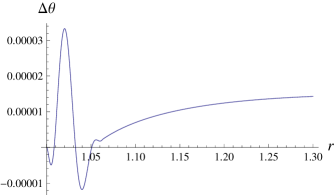
The oscillatory pattern of the higher order effects are clearly present just as in the Minkowski embedding case, and before decaying eventually, the curve change its sign 3 times. This can not be seen on Fig. 5 as the amplitude is decaying very rapidly and the second and third sign change takes place further away from the horizon.

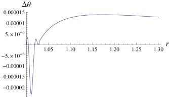
As we increase the $\theta_{0}$ parameter from $\tfrac{\pi}{900}$ to $\tfrac{\pi}{2}$ (i.e. changing the initial position of the brane on the horizon from the near pole region to the equator) the shapes and the maximum of the corresponding $\Delta\theta$ curves are changing. The tendency in these features is not so simple as in the Minkowski embedding case, for example there are several local extrema of the maximum with respect to $\theta_{0}$. Nevertheless, to illustrate some of the solutions, we picked out three examples with initial parameters $\theta_{0}\sim\tfrac{\pi}{6}$, $\tfrac{\pi}{3}$ and $\tfrac{\pi}{2}$. The corresponding curves are plotted on Figs. 6, 7 and 8, respectively.

Figure 6: The $\Delta\theta$ function in the black hole embedding case with $\theta_{0}\simeq\tfrac{\pi}{6.6}$.

Figure 7: The $\Delta\theta$ function in the black hole embedding case with $\theta_{0}\simeq\tfrac{\pi}{2.85}$.

Figure 8: The $\Delta\theta$ function in the black hole embedding case with $\theta_{0}\simeq\tfrac{\pi}{2.2}$.

For all curves in the black hole embedding case, the normalization has been calculated according to the length scale parameter corresponds to $\theta_{0}=\tfrac{\pi}{900}$.

VIII Quasi-static phase transition

Having in hand the exact numerical solution of the curvature corrected BBH problem, we are in the position to analyze the topology changing transition between the black hole and Minkowski embedding phases by considering the energy properties of a quasi-static brane evolution from an initially equatorial configuration. This method has been introduced first by Flachi et al. in Flachi (20), and its details for our purposes have been explained in CF (1).

The idea is very simple, one compares the energy of a thick brane configuration that belongs to a chosen initial parameter $\theta_{0}$ (in the black hole embedding case) or $r_{1}$ (in the Minkowski embedding case) to the energy of the equatorial configuration, i.e. to the brane with $\theta_{0}=\tfrac{\pi}{2}$. If one plots the energy difference $\Delta E$ introduced this way as a function of the cylindrical distance parameter defined as

$$Z_{\infty}=r_{\infty}\cos\theta(r_{\infty})$$

(where $r_{\infty}$ denotes a certain cut off distance very far from the horizon) for every initial parameter $\theta_{0}$ and $r_{1}$, then the obtained plot exhibits a loop, or instability zone, that is a typical sign of a first order phase transition in dynamical systems. For further details please refer to CF (1) or Flachi (20).

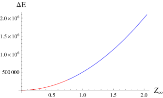
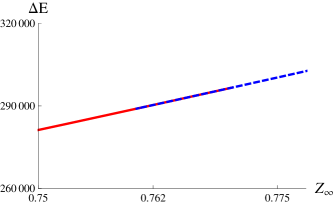
In Fig. 9 we have plotted the $\Delta E(Z_{\infty})$ curves for the presented 5-dimensional brane solutions in a 6-dimensional bulk. The red curve represents the evolution of the brane in the black hole embedding phase, while the blue belongs to the evolution in the Minkowski embedding phase. It can be seen on the picture that something interesting happens around $Z_{\infty}\simeq 0.8$, where the two curves seems to touch each other.

Figure 9: The picture shows the $\Delta E(Z_{\infty})$ curves of a quasi-static thick brane evolution in the case of a 5-dimensional brane in a 6-dimensional bulk. The red curve belongs to the black hole embedding-, while the blue curve to the Minkowski embedding evolution.

If we enlarge this part on Fig. 10, it becomes apparent that indeed the two curves overlap in the $0.76\lesssim Z_{\infty}\lesssim 0.77$ interval, which clearly shows that there is an energy degeneracy in the brane evolution at the near singularity region. In fact this overlap exhibits a real one-dimensional loop in the sense that both curves has a turn-back point in this region. The black hole embedding (red) curve increases from zero until it reaches its maximum around $Z_{\infty}\simeq 0.77$, where it turns back and start decreasing and converges to some point in the overlap region. The Minkowski embedding (blue) curve starts decreasing from the same point (this point represents the curvature singularity) until $Z_{\infty}\simeq 0.76$, where it turns back and starts increasing to infinity. Unfortunately, since being a one-dimensional loop, it can not be seen on the graph.

Figure 10: The enlargement of the overlap region on Fig. 9.

In any case, the above property of the brane evolution demonstrates that the corresponding topology changing transition remains a first order one in the curvature corrected BBH system, just as it was in the infinitely thin case.

IX Conclusions

In the present paper we further studied the effects of higher order, curvature corrections to the dynamics of higher dimensional brane black hole systems. Since earlier results CF (1, 6) clearly showed that perturbative approaches fail to provide regular solutions near the axis of the system in Minkowski type topologies, we considered a different, exact, numerical approach to the problem. We analyzed the asymptotic properties of the complete $4th$-order equation of motion of the thick BBH system, provided its asymptotic solution for far distances, and obtained regularity conditions in the near horizon region for both Minkowski and black hole embeddings.

We showed that the requirement of regularity for the thick solution defines almost completely the boundary conditions for the Euler-Lagrange equation in the Minkowski embedding case. The only exceptions are the brane configurations with 1, 2 and 3 spacelike dimensions. In the case of 1 and 3 spacelike dimensions regular solutions of the problem exist, however, which is an unexpected result, with 2 spaclike dimensions the problem can not be solved with the applied method. Nevertheless it is obvious that the lack of a regular solution in this case should not have any physical reason as a regular perturbative solution clearly exist in accordance with explicitly constructed field theoretical domain wall solutions Fl1 (16, 17) to the problem.

For the black hole embedding solutions, the boundary conditions are not completely determined form the regularity requirements, nevertheless, since the perturbative approach, presented in CF (1), is valid for this case, the missing conditions can be borrowed from those results.

Having in hand all the boundary conditions we provided a set of exact, numerical solutions in the near horizon region for both Minkowski and black hole topologies in the case when a 5-dimensional brane embedded into a 6-dimensional bulk. Based on the obtained solutions we discussed the properties of a topology changing transition in the system, and concluded that the transition remains first order just as it was in the thin model.

The main results of the paper are the construction of the exact numerical solution for the thick BBH problem in any dimensions (apart from the $n=1$ special case), and the clarification of the question whether the simplest, higher order, curvature corrections can modify the order of the phase transition in the system.

The obtained results are relevant in several research areas that are considering similar setup to the BBH system. A few of them were mentioned in the introduction section.

Appendix A Coefficient Functions

$$T_{2} = \frac{1}{64(a+b)\varepsilon f^{2}r^{4}F^{4}}\left[\right.-8\dot{\theta}^{9}\varepsilon f^{6}(a+b+an)(-1+n^{2})r^{9}$$

$$- 2\dot{\theta}^{2}f^{4}r^{5}(240(a+b)\ddot{\theta}^{2}\dot{\theta}\varepsilon(-3+n)r^{2}-480(a+b)\ddot{\theta}^{3}\varepsilon r^{3}+8\ddot{\theta}\dot{\theta}^{2}\varepsilon r(-71(a+b)$$

$$+ 45an+42bn+2(a-2b)n^{2}+24(a+b)\ddot{\theta}nr^{2}\cot\theta)+4\dot{\theta}^{3}\varepsilon(b(-80+(69-7n)n)$$

$$+ a(-80+n(54+(29-3n)n))+2\ddot{\theta}(a(37-17n)+b(25-8n))nr^{2}\cot\theta)$$

$$+ 4\dot{\theta}^{6}nr^{3}\cot\theta(2\varepsilon n(b-an)-r^{2}+\varepsilon r(-3\dot{f}(a+2b+3an)-4a\ddot{f}r)$$

$$- 2\varepsilon(b-a(-2+n))(-2+n)\csc\theta^{2})+4\dot{\theta}^{5}r^{2}(\varepsilon n(-a(-25+n)n+b(-3+11n))$$

$$+ (5+4n)r^{2}+\varepsilon r(\dot{f}(2b(8+n)+a(13+n(27+5n)))+r(\ddot{f}(5a-3b-2an)-2af^{(3)}r))$$

$$+ \varepsilon n(b(13-11n)+a(28+(-27+n)n))\csc\theta^{2})+4\dot{\theta}^{4}r(\varepsilon n(b(57-31n)$$

$$+ a(89-n(26+19n)))\cot\theta+\ddot{\theta}r^{2}(2\varepsilon n(5an+b(-1+4n))+r^{2}+\varepsilon r(3\dot{f}(a+2b+3an)$$

$$+ 4a\ddot{f}r)+2\varepsilon(a(6-5n)+b(5-4n))n\csc\theta^{2}))+\dot{f}\dot{\theta}^{7}r^{5}((3a+b)\dot{f}\varepsilon(1+n)r+2(2a\varepsilon n^{2}$$

$$+ r^{2}+(a+b)\ddot{f}\varepsilon r^{2}-2a\varepsilon(-1+n)n\csc\theta^{2})))+2f^{2}r(3(2a+b)\dot{f}^{3}\dot{\theta}^{7}\varepsilon r^{9}$$

$$- 23(a+b)\dot{f}^{2}\dot{\theta}^{6}\varepsilon nr^{7}\cot\theta+8\ddot{\theta}\varepsilon r(a(2+n)(4+5n)+b(8+n(15+4n))$$

$$+ 6(a+b)\ddot{\theta}nr^{2}\cot\theta)+8\dot{\theta}\varepsilon(n^{2}(3b+a(2+n))-90(a+b)\ddot{\theta}^{2}\dot{f}r^{5}+\ddot{\theta}n(b(25+8n)$$

$$+ a(28+17n))r^{2}\cot\theta)-2\dot{f}\dot{\theta}^{5}r^{5}(2(a+4b)\varepsilon n^{2}+9r^{2}+3\varepsilon r(\dot{f}(5b(-1+n)+a(4+11n))$$

$$+ 8(a+b)\ddot{f}r)-2(a+4b)\varepsilon(-1+n)n\csc\theta^{2})+4\dot{\theta}^{3}r^{2}(\varepsilon n(b(3-9n)+an(-21+19n))$$

$$+ (-7-4n)r^{2}+\varepsilon r(2r(\ddot{f}(b(9+4n)+2a(5+7n))+(5a+2b)f^{(3)}r)+\dot{f}(2(b(-78$$

$$+ n(13+2n))+2a(-42+n(-5+6n)))+(47a+26b)\ddot{\theta}nr^{2}\cot\theta))-\varepsilon(-1+n)n(-9b$$

$$+ a(-24+19n))\csc\theta^{2})+2\dot{\theta}^{4}r^{3}(3(7a+10b)\ddot{\theta}\dot{f}^{2}\varepsilon r^{4}+2\varepsilon nr(\dot{f}(b(47+8n)+a(74+53n))$$

$$+ 4(5a+2b)\ddot{f}r)\cot\theta+6n\cot\theta(\varepsilon n(-3b+an)+2r^{2}+\varepsilon(3b-a(-4+n))(-2+n)\csc\theta^{2}))$$

$$+ 4\dot{\theta}^{2}r(\varepsilon n(21bn+a(-6+n(50+n)))\cot\theta+\ddot{\theta}r^{2}(4(a-2b)\varepsilon n^{2}-3r^{2}+6\varepsilon r(\dot{f}(a(-48+n)$$

$$+ b(-46+3n))+(a+b)\ddot{f}r)-4(a-2b)\varepsilon(-1+n)n\csc\theta^{2})))-4\dot{\theta}^{6}f^{5}r^{7}(2\dot{\theta}\varepsilon(a+b$$

$$+ an)(-24+n(17+n))+2\ddot{\theta}\varepsilon(-13+7n)(a+b+an)r-2\dot{\theta}^{2}\varepsilon n(-13+7n)(a+b$$

$$+ an)r\cot\theta+\dot{\theta}^{3}r^{2}(\varepsilon(1+n)r(\dot{f}(3(a+b)+5an)+2a\ddot{f}r)+2(2\varepsilon n^{2}(a+b+an)$$

$$+ (1+n)r^{2}-2\varepsilon(-1+n)n(a+b+an)\csc\theta^{2})))-2f(-9(2a+3b)\dot{f}^{3}\dot{\theta}^{5}\varepsilon r^{8}$$

$$- 8\varepsilon(b-a(-2+n))(-1+n)n\cot\theta+2(-17a+4b)\dot{f}^{2}\dot{\theta}^{4}\varepsilon nr^{6}\cot\theta-4\ddot{\theta}r^{2}(-r^{2}$$

$$+ 2\varepsilon r(\dot{f}(20a(2+n)+b(40+17n))+(10a+9b)\ddot{f}r)+\varepsilon n(b-7an)\cot\theta^{2}+8a\varepsilon n\csc\theta^{2})$$

$$- 4\dot{\theta}r(\varepsilon n^{2}(-b+7an)+(-2-n)r^{2}+2\varepsilon r(r(2\ddot{f}(3a(2+n)+b(5+n))+(2a+b)f^{(3)}r)$$

$$+ \dot{f}(2a(2+n)(2+3n)+b(8+n(15+n))+(28a+19b)\ddot{\theta}nr^{2}\cot\theta))+\varepsilon(b$$

$$+ a(8-7n))n^{2}\csc\theta^{2})+2\dot{f}\dot{\theta}^{3}r^{4}(\varepsilon n(-21an+b(3+4n))+7r^{2}+\varepsilon r(\dot{f}(2a(62+n)$$

$$+ b(102+7n))+12b\ddot{f}r)+\varepsilon n(b-4bn+3a(-8+7n))\csc\theta^{2})-2\dot{\theta}^{2}r^{2}(-3(46a+43b)\ddot{\theta}\dot{f}^{2}\varepsilon r^{4}$$

$$+ 2n\cot\theta(-\varepsilon n(5b+an)+4r^{2}+\varepsilon r(\dot{f}(74a+41b+4(4a+b)n)+(5a+4b)\ddot{f}r)$$

$$+ \varepsilon(-2+n)(5b+a(4+n))\csc\theta^{2})))+f^{3}r^{3}(-480(a+b)\ddot{\theta}^{2}\dot{\theta}\varepsilon(4+n)r^{2}$$

$$- 160(a+b)\ddot{\theta}^{3}\varepsilon r^{3}+(a+b)\dot{f}^{3}\dot{\theta}^{9}\varepsilon r^{9}-2(5a+b)\dot{f}^{2}\dot{\theta}^{8}\varepsilon nr^{7}\cot\theta$$

$$- 8\ddot{\theta}\dot{\theta}^{2}\varepsilon r(b(240+(47-16n)n)+a(240+(68-13n)n)+36(a+b)\ddot{\theta}nr^{2}\cot\theta)$$

$$+ 8\dot{\theta}^{3}\varepsilon(b(-48+13(-4+n)n)+a(2+n)(-24+n(-18+5n))+30(a+b)\ddot{\theta}^{2}\dot{f}r^{5}$$

$$+ 2\ddot{\theta}n(16bn+a(-9+34n))r^{2}\cot\theta)+8\dot{\theta}^{4}r(\varepsilon n(b(-42+43n)+a(-78+n(76+15n)))\cot\theta$$

$$- \ddot{\theta}r^{2}(16(a+b)\varepsilon n+3r^{2}+\varepsilon r(\dot{f}(-14a-23b+43an+16bn)+6(3a+2b)\ddot{f}r)$$

$$+ \varepsilon(b(19-16n)+a(16-13n))n\cot\theta^{2}))+2\dot{\theta}^{6}r^{3}((5a+b)\ddot{\theta}\dot{f}^{2}\varepsilon r^{4}+4n\cot\theta(-7b\varepsilon n+5a\varepsilon n^{2}$$

$$+ 4r^{2}+\varepsilon r(\dot{f}(2b(7+2n)+7a(1+6n))+(17a+4b)\ddot{f}r)+\varepsilon(7b+a(12-5n))(-2+n)\csc\theta^{2}))$$

$$+ 2\dot{f}\dot{\theta}^{7}r^{5}(\varepsilon r(\dot{f}(-5b(2+n)-a(14+25n))-2(9a+5b)\ddot{f}r)+2(\varepsilon n(b-11an-4bn)-5r^{2}$$

$$+ \varepsilon n(b(-5+4n)+a(-12+11n))\csc\theta^{2}))-4\dot{\theta}^{5}r^{2}(\varepsilon r(-2\ddot{f}(-8a+b+19an+4bn)r$$

$$- 4(4a+b)f^{(3)}r^{2}+\dot{f}(a(76+(150-19n)n)+b(58+(9-4n)n)+6(3a+4b)\ddot{\theta}nr^{2}\cot\theta))$$

$$+ 2(\varepsilon n(a(44-15n)n+b(-6+17n))+(9+6n)r^{2}+\varepsilon n(b(20-17n)$$

$$+ a(50+n(-62+15n)))\csc\theta^{2})))+4(-2(10a+7b)\dot{f}^{3}\dot{\theta}^{3}\varepsilon r^{6}+\dot{f}^{2}\varepsilon r^{3}(2(18a+17b)\ddot{\theta}r$$

$$+ \dot{\theta}(20a(2+n)+6b(6+n)+(26a+7b)\dot{\theta}nr\cot\theta))+2n\cot\theta(-\varepsilon n(b+an)+r^{2}-2a\ddot{f}\varepsilon r^{2}$$

$$+ \varepsilon(-2+n)(b+an)\csc\theta^{2})+2\dot{f}r(2\varepsilon n(2a+b-2an)\cot\theta$$

$$+ \dot{\theta}r(-r^{2}+4(2a+b)\ddot{f}\varepsilon r^{2}+\varepsilon n((b-7an)\cot\theta^{2}+8a\csc\theta^{2}))))\left.\right]$$

$$s_{3} = \frac{1}{8(a+b)r^{4}f^{2}}\left[n(n-2)(1+r^{2}f\dot{\theta}^{2})(b+an+2(b-a(n-2))r^{2}f\dot{\theta}^{2})\right]\ ,$$ (31)

$$s_{2} = \frac{1}{16(a+b)r^{3}f^{2}}\left[n(2\dot{f}\dot{\theta}(b+a(8-7n))r+4\dot{\theta}^{5}f^{3}(n-1)(a+b+an)r^{4}\right.$$

$$+ f(2\dot{\theta}n(8a+b-7an)+2\ddot{\theta}(8a+b-7an)r+\dot{f}\dot{\theta}^{3}(7an+4bn-8a-5b)r^{3})$$

$$+ 2\dot{\theta}^{2}f^{2}r^{2}(2\ddot{\theta}(b(4n-5)+a(5n-6))r+\dot{\theta}(b(7n-9)+a((27-5n)n-24)$$

$$+ \left.a\dot{f}\dot{\theta}^{2}(n-1)r^{3})))\right]\ ,$$

$$s_{1} = \frac{1}{32(a+b)r^{4}\varepsilon f^{2}F^{2}}\left[n(-4\varepsilon n(b+an)+4r^{2}+4\dot{\theta}^{6}\varepsilon f^{4}(-13+7n)(a+b+an)r^{6}\right.$$

$$+ 2\varepsilon r(-4a\ddot{f}r+\dot{f}(8a+4b-8an+(26a+7b)\dot{f}\dot{\theta}^{2}r^{3}))+4\dot{\theta}^{2}f^{3}r^{4}(4\dot{\theta}^{2}\varepsilon(b(-11+6n)$$

$$+ a(-19+n(8+3n)))-48(a+b)\ddot{\theta}^{2}\varepsilon r^{2}+2\dot{\theta}\varepsilon r(\ddot{\theta}(-37a-25b+17an+8bn)$$

$$+ 8(a+b)\theta^{(3)}r)+\dot{\theta}^{4}r^{2}(2\varepsilon n(-b+an)+r^{2}+\varepsilon r(3\dot{f}(a+2b+3an)+4a\ddot{f}r)))$$

$$+ f^{2}r^{2}(4\dot{\theta}^{2}\varepsilon(b(2+19n)+a(-2+n(44+3n)))+48(a+b)\ddot{\theta}^{2}\varepsilon r^{2}$$

$$- 12(3a+4b)\ddot{\theta}\dot{f}\dot{\theta}^{3}\varepsilon r^{4}-(5a+b)\dot{f}^{2}\dot{\theta}^{6}\varepsilon r^{6}+8\dot{\theta}\varepsilon r(\ddot{\theta}(28a+25b+17an+8bn)$$

$$+ 8(a+b)\theta^{(3)}r)+4\dot{\theta}^{4}r^{2}(\varepsilon n(-5b+3an)+3r^{2}+\varepsilon r(\dot{f}(4b(2+n)+a(4+33n))$$

$$+ (13a+4b)\ddot{f}r)))+2f(4\varepsilon(b-a(-2+n))(-1+n)+\dot{\theta}r^{2}(4(28a+19b)\ddot{\theta}\dot{f}\varepsilon r^{2}$$

$$+ \dot{\theta}(-8b\varepsilon n+6r^{2}+\varepsilon r(2(7a+4b)\ddot{f}r+\dot{f}(78b+8bn+20a(7+2n)$$

$$- (9a+11b)\dot{f}\dot{\theta}^{2}r^{3}))))))\left.\right]\ ,$$

$$g(\dot{\theta}|_{r_{1}}) = -((\dot{\theta}(2(b+a(8-7n))(fn+\dot{f}r)+2\dot{\theta}^{4}f^{2}(-1+n)r^{4}(2f(a+b+an)+a\dot{f}r)$$

$$+ \dot{\theta}^{2}fr^{2}(-2f(b(9-7n)+a(24+n(-27+5n)))+\dot{f}(b(-5+4n)$$

$$+ a(-8+7n))r)))/(2fr(b+a(8-7n)+2\dot{\theta}^{2}f(b(-5+4n)$$

$$+ a(-6+5n))r^{2})))\left.\right|_{r_{1}}\ ,$$

$$h(\dot{\theta}|_{r_{1}},\ddot{\theta}|_{r_{1}}) = \frac{1}{64(a+b)\dot{\theta}\varepsilon f^{2}r^{4}F^{2}}\left[\right.(4\varepsilon n(b+an)-4r^{2}$$

$$- 4\dot{\theta}^{6}\varepsilon f^{4}(-13+7n)(a+b+an)r^{6}+2\varepsilon r(4a\ddot{f}r+\dot{f}(-4b+8a(-1+n)$$

$$- (26a+7b)\dot{f}\dot{\theta}^{2}r^{3}))-4\dot{\theta}^{2}f^{3}r^{4}(4\dot{\theta}^{2}\varepsilon(b(-11+6n)+a(-19+n(8+3n)))$$

$$+ 2\ddot{\theta}\dot{\theta}\varepsilon(b(-25+8n)+a(-37+17n))r-48(a+b)\ddot{\theta}^{2}\varepsilon r^{2}$$

$$+ \dot{\theta}^{4}r^{2}(2\varepsilon n(-b+an)+r^{2}+\varepsilon r(3\dot{f}(a+2b+3an)+4a\ddot{f}r)))$$

$$+ 2f(-4\varepsilon(b-a(-2+n))(-1+n)-4(28a+19b)\ddot{\theta}\dot{f}\dot{\theta}\varepsilon r^{4}$$

$$+ (9a+11b)\dot{f}^{2}\dot{\theta}^{4}\varepsilon r^{6}-2\dot{\theta}^{2}r^{2}(-4b\varepsilon n+3r^{2}+\varepsilon r(\dot{f}(70a+39b+4(5a+b)n)$$

$$+ (7a+4b)\ddot{f}r)))+f^{2}r^{2}(-4\dot{\theta}^{2}\varepsilon(b(2+19n)+a(-2+n(44+3n)))$$

$$- 8\ddot{\theta}\dot{\theta}\varepsilon(b(25+8n)+a(28+17n))r-48(a+b)\ddot{\theta}^{2}\varepsilon r^{2}+12(3a+4b)\ddot{\theta}\dot{f}\dot{\theta}^{3}\varepsilon r^{4}$$

$$+ (5a+b)\dot{f}^{2}\dot{\theta}^{6}\varepsilon r^{6}-4\dot{\theta}^{4}r^{2}(\varepsilon n(-5b+3an)+3r^{2}+\varepsilon r(\dot{f}(4b(2+n)$$

$$+ a(4+33n))+(13a+4b)\ddot{f}r))))\left.\right]\left.\right|_{r_{1}}\ ,$$

$$y_{2} = \frac{1}{16(a+b)\varepsilon r^{4}}\left[\right.-2(10a+7b)\dot{f}^{3}\dot{\theta}^{3}\varepsilon r^{6}+\dot{f}^{2}\varepsilon r^{3}(2(18a+17b)\ddot{\theta}r+\dot{\theta}(20a(2+n)$$

$$+ 6b(6+n)+(26a+7b)\dot{\theta}nr\cot\theta))+2n\cot\theta(r^{2}-2a\ddot{f}\varepsilon r^{2}$$

$$+ \varepsilon(b+an)(-n+(-2+n)\csc^{2}\theta))+2\dot{f}r(2\varepsilon(b-2a(-1+n))n\cot\theta$$

$$+ \dot{\theta}r(-r^{2}+4(2a+b)\ddot{f}\varepsilon r^{2}+\varepsilon n((b-7an)\cot^{2}\theta+8a\csc^{2}\theta)))\left.\right]\left.\right|_{r_{0}}\ ,$$

$$y_{1} = \frac{1}{32(a+b)\varepsilon r^{4}}\left[\right.(98a+83b)\dot{f}^{3}\dot{\theta}^{5}\varepsilon r^{8}-2(35a+18b)\dot{f}^{2}\dot{\theta}^{4}\varepsilon nr^{6}\cot\theta$$

$$+ 4\dot{\theta}r(\varepsilon n^{2}(-b+7an)+(-2-n)r^{2}+2\varepsilon r(r(2\ddot{f}(3a(2+n)+b(5+n))$$

$$+ (2a+b)f^{(3)}r)+\dot{f}(2a(2+n)(2+3n)+b(8+n(15+n))$$

$$+ (28a+19b)\ddot{\theta}nr^{2}\cot\theta))+\varepsilon(b+a(8-7n))n^{2}\csc^{2}\theta)$$

$$+ 2\dot{f}\dot{\theta}^{3}r^{4}(\varepsilon n(b-7an-4bn)-3r^{2}+\varepsilon r(\dot{f}(-6a(34+7n)-b(174+19n))$$

$$- 4(8a+7b)\ddot{f}r)+\varepsilon n(b(-5+4n)+a(-8+7n))\csc^{2}\theta)$$

$$+ 2\dot{\theta}^{2}r^{2}(-(210a+197b)\ddot{\theta}\dot{f}^{2}\varepsilon r^{4}+2n\cot\theta(\varepsilon n(-3b+an)+2r^{2}$$

$$+ \varepsilon r(\dot{f}(66a+37b+4(6a+b)n)+(9a+4b)\ddot{f}r)$$

$$+ \varepsilon(3b-a(-4+n))(-2+n)\csc^{2}\theta))+4(32(a+b)\theta^{(3)}\dot{f}\varepsilon r^{4}$$

$$+ 2\varepsilon(b-a(-2+n))(-1+n)n\cot\theta+\ddot{\theta}r^{2}(-r^{2}+2\varepsilon r(\dot{f}(20a(2+n)$$

$$+ b(40+17n))+(10a+9b)\ddot{f}r)+\varepsilon n((b-7an)\cot^{2}\theta+8a\csc^{2}\theta)))\left.\right]\left.\right|_{r_{0}}\ ,$$

$$G(\dot{\theta}|_{r_{0}}) = \frac{1}{2(18a+17b)\dot{f}^{2}\varepsilon r^{4}}\left[\right.2(10a+7b)\dot{f}^{3}\dot{\theta}^{3}\varepsilon r^{6}-\dot{f}^{2}\dot{\theta}\varepsilon r^{3}(20a(2+n)+6b(6+n)$$

$$+ (26a+7b)\dot{\theta}nr\cot\theta)+2n\cot\theta(\varepsilon n(b+an)-r^{2}+2a\ddot{f}\varepsilon r^{2}-\varepsilon(-2+n)(b+an)\csc^{2}\theta)$$

$$+ 2\dot{f}r(-2\varepsilon n(2a+b-2an)\cot\theta+\dot{\theta}r(\varepsilon n(b-7an)+r^{2}-4(2a+b)\ddot{f}\varepsilon r^{2}$$

$$+ \varepsilon n(-8a-b+7an)\csc^{2}\theta))\left.\right]\left.\right|_{r_{0}}\ ,$$

$$H(\dot{\theta}|_{r_{0}},\ddot{\theta}|_{r_{0}}) = -\frac{1}{128(a+b)\dot{f}r^{4}}\left[\right.8(b-a(-2+n))(-1+n)n\cot\theta+(1/\varepsilon)r((98a+83b)\dot{f}^{3}\dot{\theta}^{5}\varepsilon r^{7}$$

$$- 2(35a+18b)\dot{f}^{2}\dot{\theta}^{4}\varepsilon nr^{5}\cot\theta+4\ddot{\theta}r(\varepsilon n(-b+7an)-r^{2}+2\varepsilon r(\dot{f}(20a(2+n)$$

$$+ b(40+17n))+(10a+9b)\ddot{f}r)+\varepsilon(b+a(8-7n))n\csc^{2}\theta)+4\dot{\theta}(\varepsilon n^{2}(-b+7an)$$

$$+ (-2-n)r^{2}+2\varepsilon r(r(2\ddot{f}(3a(2+n)+b(5+n))+(2a+b)f^{(3)}r)+\dot{f}(2a(2+n)(2+3n)$$

$$+ b(8+n(15+n))+(28a+19b)\ddot{\theta}nr^{2}\cot\theta))+\varepsilon(b+a(8-7n))n^{2}\csc^{2}\theta)$$

$$+ 2\dot{f}\dot{\theta}^{3}r^{3}(\varepsilon n(b-7an-4bn)-3r^{2}+\varepsilon r(\dot{f}(-6a(34+7n)-b(174+19n))$$

$$- 4(8a+7b)\ddot{f}r)+\varepsilon n(b(-5+4n)+a(-8+7n))\csc^{2}\theta)+2\dot{\theta}^{2}r(-(210a+197b)\ddot{\theta}\dot{f}^{2}\varepsilon r^{4}$$

$$+ 2n\cot\theta(\varepsilon n(-3b+an)+2r^{2}+\varepsilon r(\dot{f}(66a+37b+4(6a+b)n)+(9a+4b)\ddot{f}r)$$

$$+ \varepsilon(3b-a(-4+n))(-2+n)\csc^{2}\theta)))\left.\right]\left.\right|_{r_{0}}\ .$$

References

• (1) V. G. Czinner and A. Flachi, Phys. Rev. D80, 104017 (2009).
• (2) P. A. M. Dirac, Proc. R. Soc. A. 268, 57 (1962).
• (3) J. Nambu, Copenhagen Summer Symposium (1970),
unpublished.
• (4) T. Goto, Prog. Theor. Phys. 46, 1560 (1971).
• (5) B. Carter and R. Gregory, Phys. Rev. D51, 5839 (1995).
• (6) V. P. Frolov and D. Gorbonos, Phys. Rev. D79, 024006 (2009).
• (7) V. P. Frolov, Phys. Rev. D74, 044006 (2006).
• (8) B. Kol, J. High Energy Phys. 10 (2005) 049.
• (9) B. Kol, Phys. Rep. 422, 119 (2006).
• (10) B. Kol, J. High Energy Phys. 10 (2006) 017.
• (11) D. Mateos, R. C. Myers and R. M. Thomson, Phys. Rev. Lett. 97, 091601 (2006).
• (12) D. Mateos, R. C. Myers and R. M. Thomson, J. High Energy Phys. 05 (2007) 067.
• (13) E. Bombieri, E. De Giorgi and E. Giusti, Inventiones Math. 7, 243 (1969).
• (14) G. Gibbons, K. Maeda and U. Miyamoto, Class. Quantum Grav. 26, 185008 (2009).
• (15) K. Hioki, U. Miyamoto and M. Nozawa, Phys. Rev. D80, 084011 (2009).
• (16) A. Flachi, O. Pujolás, M. Sasaki and T. Tanaka, Phys. Rev. D73, 125017 (2006).
• (17) A. Flachi and T. Tanaka, Phys. Rev. D76, 025007 (2007).
• (18) A. Flachi and T. Tanaka, Phys. Rev. Lett. 95, 161302 (2005).
• (19) F. R. Thangerlini, Nuovo Cimento 77, 636 (1963).
• (20) A. Flachi, O. Pujolás, M. Sasaki and T. Tanaka Phys. Rev. D74, 045013 (2006).
• (21) C. M. Bender and S. A. Orszag, Advanced Mathematical Methods for Scientists and Engineers, McGraw-Hill, Inc. 1978.