Apparent high metallicity in 3-4 keV galaxy clusters:
the inverse iron-bias in action in the case of the merging cluster Abell 2028

Abstract

Context. Recent work based on a global measurement of the ICM properties finds evidence for an increase in the iron abundance in galaxy clusters with temperatures around 2-4 keV up to a value about 3 times higher than is typical of very hot clusters $Z_{Fe}\simeq 0.25Z_{\odot}$.

Aims. We have started a study of the metal distribution in nearby X–ray luminous poor galaxy clusters in the temperature range 3-4 keV with measured high abundances. Our study aims at spatially resolving the metal content of the central regions of the ICM, in particular characterizing how our measurements are biased by the diagnostics adopted and by the possible multi-temperature nature of the projected observed spectra. We report here on a 42ks XMM-Newton observation of the first object in the sample, the cluster Abell 2028.

Methods. We selected interesting regions of the ICM to analyze the spatially resolved structure of projected temperature and abundance, thereby producing two-dimensional maps.

Results. The XMM-Newton observation of the first object of the sample, the cluster Abell 2028, reveals the complex structure of the cluster over a scale of $\sim 300$ kpc, showing an interaction between two subclusters in cometary-like configurations. Cold fronts have been detected at the leading edges of the two substructures. The core of the main subcluster is likely hosting a cool corona. We show that a one-component fit for this region returns a biased high metallicity. The inverse iron bias is caused by the behavior of the fitting code in shaping the Fe-L complex. In the presence of a multi-temperature structure of the ICM, the best-fit metallicity turns out to be artificially higher when the projected spectrum is modeled with a single temperature component, while it is not related to the presence of both Fe-L and Fe-K emission lines in the spectrum. After accounting for the inverse iron bias, the overall abundance of the cluster is consistent with the one typical of hotter, more massive clusters.

Conclusions. We caution against interpreting high abundances inferred when fitting a single thermal component to spectra derived from relatively large apertures in 3-4 keV clusters, because the inverse iron bias can be present. Most of the inferences trying to relate high abundances in 3-4 keV clusters to fundamental physical processes will probably have to be revised.

1 Introduction

Clusters of galaxies have established themselves as a unique environment for measuring elemental abundances and for studying the chemical enrichment history of the Universe. Their large potential well retains all the metals produced by their member galaxies, allowing in principle a unified description of the thermodynamical properties of the hot phase (the diffuse X-ray emitting gas) and of the cold phase (the cluster galaxies). Indeed, the distribution of metals in the ICM is a direct consequence of the past history of star formation in the cluster galaxies and of the processes responsible for injecting enriched gas into the ICM. (For recent reviews of the observational and theoretical aspects, see Werner et al. 2008; Borgani et al. 2008; Schindler & Diaferio 2008, and references therein.)

Most of the appeal of the X-rays determining elemental abundances in the hot gas stems from the apparent robustness of the measurement: most of the observed emission lines arise from well understood hydrogen- and helium- like ions and their equivalent widths can be, under the reasonable assumption of collisional equilibrium, directly converted into the elemental abundance of the corresponding element. If some concerns arose for the reliability of the Fe-L shell modeling (e.g. Renzini 1997; Arimoto et al. 1997), it has been shown that this is not a particular issue (Buote & Fabian 1998; Buote et al. 2003b)

Unfortunately this intrinsic simplicity of the measurement has faced the limitations of the X-ray satellites in terms of the shape of the instrumental response, bandpass, and spectral and spatial resolution leading to observational biases. Correct modeling of the temperature structure is crucial, in particular when dealing with spectra extracted from a large aperture centered on the core of clusters and groups. Given the presence of strong and opposite gradients in the temperature and metallicity profiles (i.e., cooler regions are more metal rich, see De Grandi & Molendi 2001), in the spectra of central regions photons coming from regions of different temperature and abundances are mixed together. These objects and these regions naturally draw the attention of X-ray observers because of their high surface brightness, thus delivering high signal-to-noise (S/N) spectra.

The first important recognition of a bias in the measurement of elemental abundances was the description of the “iron bias” (Buote & Fabian 1998; Buote 2000a, b). Many ASCA studies found significant subsolar values for the iron abundance in groups and elliptical galaxies (e.g. Davis et al. 1999; Matsumoto et al. 1997), generally less than the stellar values in these systems and less than those observed in galaxy clusters. Buote (2000b) demonstrated that this was a bias resulting from fitting with a simple single-temperature a multi-temperature plasma, resulting in best-fitting elemental abundances that are too low. The typical ASCA spectrum for these objects was extracted from a large aperture in the core because of the large point spread function (PSF) of its telescope. Since the description of this bias, and with the help of the quantum leap increase in the quality of data with XMM-Newton and Chandra, this kind of error has been recognized and made less severe. The best-fitted abundances in the multi-phase cooling core regions of clusters and in groups have been shown to increase when two-temperature models or more complicated DEM models are used (e.g. Molendi & Gastaldello 2001; Buote et al. 2003b; Humphrey & Buote 2006; Werner et al. 2006; Matsushita et al. 2007). These new determinations helped to mitigate some of the trend seen in a plot of iron-mass-to-light ratios (IMLR) versus cluster temperature, which seem to drop by almost three orders of magnitude below 1 keV (Renzini 1997).

Another trend in the ICM abundance versus cluster temperature has been shown with increasing evidence in recent years. Using the ASCA archive observations of 273 objects Baumgartner et al. (2005) showed that clusters with gas temperature between 2 and 4 keV have a typical mean abundance that is larger by up to a factor of 3 than hotter systems. Investigating a sample of 56 clusters with Chandra at $z\gtrsim 0.3$, Balestra et al. (2007) confirms the trend of the Fe abundance with cluster temperature also in the higher redshift clusters. The observed trend may reflect a more efficient star formation in smaller clusters, as also suggested by optical and near–infrared observations of nearby systems (Lin et al. 2003; Gonzalez et al. 2007). On the contrary it may be argued that it is difficult to conceive a physical mechanism responsible for making clusters in the 3-4 keV range so unique a mass scale for chemical enrichment (see for example discussions in Renzini 1997, 2004) and that some plausible measurement bias might be in action, which has to work in the opposite way to the know Fe bias; i.e, it has to bias iron abundances high. A fundamental step has been made in this direction by Rasia et al. (2008), who analyzed mock XMM-Newton observations of simulated galaxy clusters finding a systematic overestimate of iron for systems in the 2-3 keV range. The reason they put forward for this discrepancy is the complex temperature structure of the simulated clusters, due to projection and low spatial resolution, and to their particular temperature range. Simionescu et al. (2009) support this explanation by analyzing a deep XMM-Newton observation of the high-luminosity cluster Hydra A finding a biased high Fe abundance at a level of 35% in the central three arcminutes, for the first time dubbing this kind of bias as the “inverse” Fe bias. This appealing solution has been suggested by Rasia et al. (2008) as a possible explanation of the Baumgartner et al. (2005) results.

With the aim of shedding more light on these issues by going beyond single-aperture measurements, we started with the present work a study of the metal distribution in iron-rich poor galaxy clusters ($3<kT_{\rm gas}<5$ keV) at redshift below $0.1$. From the work of Baumgartner et al. (2005), we selected the objects whose measurements lie at the highest end of the metal distribution. Here we present the analysis of the XMM-Newton observation of Abell 2028, the first object in the sample.

Abell 2028 is a Bautz-Morgan type II-III galaxy cluster of Richness Class 1 located at redshift 0.0777 (Struble & Rood 1999). At this redshift 1 arcmin corresponds to 88 kpc. The Galactic absorption in the cluster’s direction is $2.46\times 10^{20}$ cm^-2 (Kalberla et al. 2005). Baumgartner et al. (2005) used ASCA to measure within an aperture of 7′ an emission-weighted temperature of $3.91\pm 0.61$ keV and metallicity of $0.77^{+1.25}_{-0.51}Z_{\odot}$ (error at the 90% c.l.).

The outline of our work is the following. In Section 2, we describe the observation and data reduction. In Section 3 we describe the morphology of the cluster and discuss the surface brightness profiles in selected regions. In Section 4 we discuss the spectral analysis and the temperature and abundances maps, highlighting the relevance of the inverse iron bias in the central region of A 2028. We discuss the results of our analysis in Section 5. We summarize our results and draw conclusions for the present study in Section 6. We show the results of simulations aiming at characterizing the inverse iron bias in the Appendix. Throughout this work, if not otherwise stated, we plot and tabulate values with errors quoted at the 68.3 per cent ($1\sigma$) level of confidence, assuming a Hubble constant $H_{0}=70h_{70}^{-1}$ km s^-1 Mpc^-1 and $\Omega_{\rm m}=1-\Omega_{\Lambda}=0.3$. All the metallicity estimates refer to the solar abundance in Anders & Grevesse (1989) just for ease of comparison with previous work, because this set of solar abundances is now outdated.

Figure 1: Mosaic of the MOS1, MOS2, and pn images in the 0.5-2 keV energy band smoothed on a 12” scale. The image has been divided by the summed exposure maps to correct for exposure variations.

2 Observation and data reduction

The cluster Abell 2028 was observed by XMM-Newton on July 29, 2007. The data were reduced with SAS v8.0 using the tasks emchain and epchain. We only considered event patterns 0-12 for MOS and 0 for pn, and the data were cleaned using the standard procedures for bright pixels and hot columns removal (by applying the expression FLAG == 0) and pn out-of-time correction. The energy scale of the pn over the whole spectral bandpass was further improved with the task epreject. Periods of high backgrounds due to soft protons were filtered using a threshold cut method by means of a Gaussian fit to the peak of the histogram of the time bins of the light curve (see Appendix A of Pratt & Arnaud 2002; De Luca & Molendi 2004) and excludede where the count rate lies more than 3$\sigma$ away from the mean. The light curves were extracted from regions of least source contamination (excising the bright object core in the central 8′ and the point source list from the SOC pipeline, after visual inspection) in two different energy bands: a hard band, 10-12 keV for MOS and 10-13 keV for pn (using 100s bins), and a wider band, 0.5-10 keV (using 10s bins), as a safety check for possible flares with soft spectra (Nevalainen et al. 2005; Pradas & Kerp 2005). The flaring periods thus determined were further checked by visual inspection of the light curves, resulting in net exposures of 40.2 ks, 38.9 ks, and 29.5 for respectively the MOS1, MOS2, and pn detectors. Point sources were detected using the task ewavelet in the energy band 0.5-10 keV and checked by eye on images generated for each detector. Detected point sources from all detectors were merged, and the events in the corresponding regions were removed from the event list, using circular regions of 25″ radius centered at the source position. The area lost by point source exclusion, CCD gaps, and bad pixels was calculated using a mask image. Redistribution matrix files (RMFs) and ancillary response files (ARFs) were generated with the SAS tasks rmfgen and arfgen, the latter in extended source mode. Appropriate flux-weighting was performed for RMFs, using our own dedicated software, and for ARFs using exposure-corrected images of the source as detector maps (with pixel size of 1′, the minimum scale modeled by arfgen) to sample the variation in emission, following the prescription of Saxton & Siddiqui (2002). For the background subtraction, we adopted a complete modeling of the various background components as described in detail in Gastaldello et al. (2007). We accurately model the actual sky background using a region free of cluster emission at $r>10$′ to the east where the signal-to-noise ratio of the surface brightness profile in the 0.5-2 keV band falls below 2. Abell 2028 is projected towards a region of enhanced Galactic background, and in agreement with previous studies (see for example the case of Abell 2029, a cluster in the same region of the sky in Vikhlinin et al. 2005), we found it necessary to add a third thermal component at $\sim 0.4$ keV. We checked the observation for contamination by solar wind charge exchange. The ACE SWEPAM proton flux was less than $4\times 10^{8}$ protons s^-1 cm^-2 which is typical of the quiescent Sun (e.g., Snowden et al. 2004; Fujimoto et al. 2007; Yoshino et al. 2009), and the light curve accumulated in a 0.5-2 keV energy band (after soft proton flares removal) did not show any variability. The spectra of the out-of-field-of-view events of CCD 4 and 5 of MOS1 and CCD 5 of MOS 2 showed an anomalously high flux in the soft band (see Kuntz & Snowden 2008) so they were therefore excluded from our analysis.

Figure 2: Left panel: Exposure-corrected MOS image in the 0.5-2 keV band with the angular sectors used to extract the surface brightness profiles shown in the other panels. Point sources were masked when extracting the profiles. The positions of the surface brightness jumps discussed in the text and shown in the next panel are indicated by arrows. Center panel: Surface brightness profiles for the selected angular sectors shown in the left panel for the main subcluster A. The radial ranges where surface brightness profiles change rapidly because of the surface brightness jumps are indicated by the shaded gray area. Right panel: same as the center panel, but for the smaller subcluster B.

3 X-ray image and surface brightness profiles

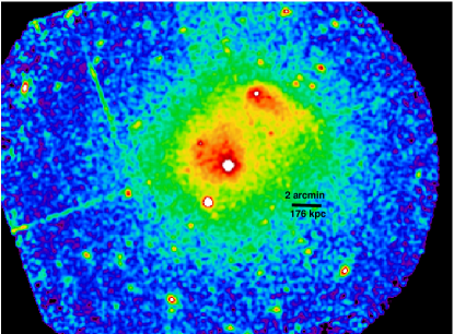
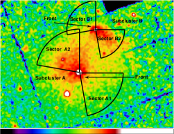
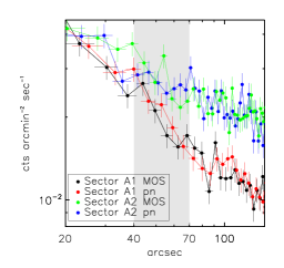
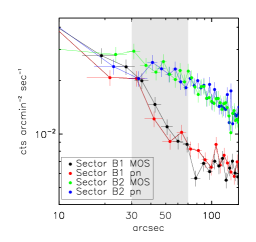
For each detector, we created images in the 0.5-2 keV band and exposure maps at the monochromatic energy of 1 keV and then combined the images into a single exposure-corrected image, smoothed on a scale of 12”, as shown in Fig.1. The X-ray emission clearly reveals two merging subclusters, a more luminous SE component (which we will call subcluster A in the following and labeled accordingly in Fig.2) and a less luminous NW one (subcluster B in the rest of the paper and labeled accordingly in Fig.2). The “cometary” shape of the two subclusters seems to suggest the direction of the merging, with the subcluster A coming from the NE direction and the subcluster B coming from SW. A further confirmation of this interpretation comes from the presence of surface brightness jumps in the suggested direction of motion of the two subclumps: we extracted from the combined MOS and pn exposure-corrected images profiles from selected angular sectors as depicted in Fig.2 centered on the surface brightness peaks of the two subclusters, with bins accumulated to have 100 counts. The surface brightness jumps are visible in the SW direction for subcluster A (sector A1, center panel of Fig.2) in the radial range 40″-70″ and in the NE direction for the subcluster B (sector B1, right panel of Fig.2) in the radial range 30″-70″. When coupled with the spectral information (see Section 4.1), these surface brightness jumps can be interpreted as merging cold fronts. For comparison plots of the profile in the direction of the tails of the two subclusters are also shown (sector A2 for subcluster A and sector B2 for subcluster B), highlighting the clear asymmetry in the surface brightness distribution of the two subclusters.

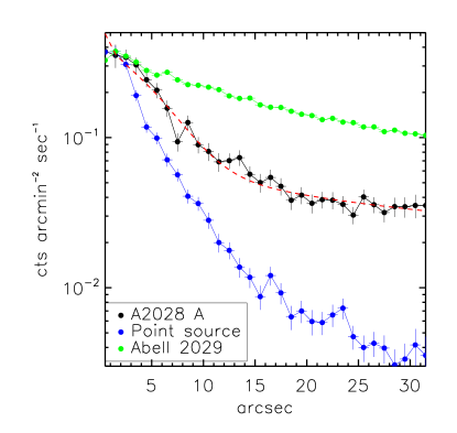
The X-ray peak location of the main subcluster A is consistent with the position of its brightest central galaxy, GIN 416. In Fig.3 we show the surface brightness profiles extracted from the combined MOS image and accumulated in bins of 1.1″ (corresponding to the MOS physical pixel size; MOS is better suited to this type of analysis because it oversamples the core of the PSF, on the contrary the pn pixel physical size is 4.1″). In the same figure we plot the profile of the bright point source (RA 15:09:34, DEC +07:30:54) SE of the main subcluster and the XMM-Newton profile of Abell 2029 (OBSID 0111270201), one of the clusters with the most peaked surface brightness profile and at the same redshift of A2028. Profiles are scaled to match their peaks of surface brightness. In the innermost 8″, the surface brightness data indicate of an excess. We fitted the inner 30″ of the A 2028 A profile with a Gaussian plus a power law, the latter component modeling the ICM emission. The best fit model, with a $\chi^{2}/\rm{dof}=29/28$ gives a width for the Gaussian of $\sigma=(4.9\pm 0.3)$″, which corresponds to an FWHM of $(11.5\pm 0.7)$″ bigger than the on-axis FWHM of the XMM-Newton PSF, which is 4.4″ for MOS at 1.5 keV. This excess central component, which is more extended than a point source, may be a corona associated with the BCG, as seen in many merging clusters (Vikhlinin et al. 2001a; Sun et al. 2007). Coronae are sources extended on kpc scales, and they are the remnants of galactic X-ray coronae with temperatures around 1 keV, compressed by the hot gas of the cluster. The spectral information we present in Section 4.2 will strengthen this interpretation.

Figure 3: Surface brightness profile of the core of subcluster A of A2028 compared to the one of the bright point source SE of the subcluster and to the A2029 cluster, one of the clusters with the most peaked surface brightness profile. The profiles have been scaled to match the peak of the radial profile of A2028 A: the point source profile was multiplied by 0.29 and the A2029 profile by 0.058. The dotted red line corresponds to the best-fit Gaussian+power-law model of the profile of the core of A 2028 A discussed in the text.

4 Spectral analysis

4.1 Temperature and abundance maps

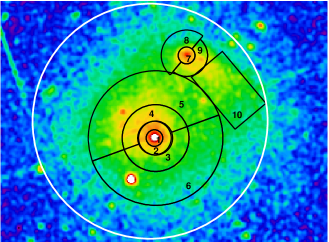
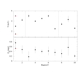
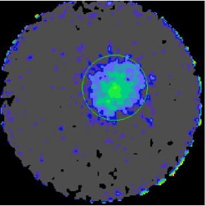
We extracted spectra in a series of regions as depicted in the left panel of Fig.4, chosen to select relevant regions of the ICM. Given the complex geometry and the relatively low number of counts we did not de-project the spectra and the results quoted in this paper come from fitting projected spectra. They consist in two concentric annular regions centered on the emission peak of the subcluster A (RA 15:09:28 DEC +07:33:20) with bounding radii 0′-0.5′, 0.5′-1′ and four sectors with bounding radii 1′-2′ and 2′-4′; a circle of 0.5′ radius centered on the emission peak of the subcluster B (RA 15:09:20 DEC +07:38:15), two sectors with bounding radii 0.5′-1′ and a box of 4′$\times$2.4′ encompassing the tail. The radii of regions 2 and 3 and of regions 7 and 8 have been determined to match the surface brightness jumps discussed in Section 3 as closely as possible, in order to investigate the temperature variation across these fronts. We fitted the background subtracted spectra with a single APEC thermal plasma model (Smith et al. 2001) in the 0.5-10 keV band with the absorbing column density fixed at the Galactic value. The temperature and abundance values of the regions of the map thus obtained are shown in the right panel of Fig.4. The temperature map reveals that subcluster A has a uniform temperature distribution in the range 4-5 keV with a drop in the inner 30″ region to 3 keV, whereas subcluster B seems to have a temperature gradient, increasing from 2 keV in the surface brightness peak to 4 keV. The abundances in every region chosen for spectral analysis show values in the range 0.3-0.5 $Z_{\odot}$, with the exception of the central 0.5′ region of subcluster A. In this region a single temperature fit returns a high metallicity of $0.76\pm 0.14$ $Z_{\odot}$. The regions corresponding to the surface brightness jumps described in Section 3 are consistent with being cold fronts, because in subcluster A the temperature increases from $4.2^{+0.2}_{-0.1}$ keV in region 2 to $5.0\pm 0.4$ keV in region 3 and in the subcluster B from $2.5\pm 0.2$ keV in region 7 to $3.4^{+0.3}_{-0.2}$ keV in region 8.

Figure 4: Left panel: Regions used for spectral extraction to derive the temperature and abundance maps. The white circle corresponds to the ASCA aperture. Right panel: Black circles correspond to the values and $1\sigma$ error bars for the temperature and abundances obtained with the 1T model for each region shown in the left panel, discussed in the text in Section 4.1. The dashed vertical lines indicate the regions adjacent to the surface brightness jumps of Figure 2. The red triangles correspond to the values for temperature and abundance obtained with a 2T model, as discussed in the text in Section 4.2. The higher temperature value at 5 keV has been fixed.

Figure 5: Left panel: X-ray spectrum of the core of the main subcluster of Abell 2028 taken from a 0.5′ aperture (corresponding to region 1 of Fig.4). Data from MOS1, MOS2, and pn are plotted in black, red, and green, respectively. The best-fit model obtained from a 1T fit in the broad band 0.5-10 keV and residuals are also shown.
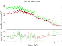
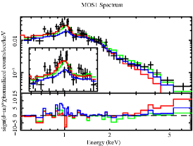
Central Panel: MOS 1 spectrum from the inner core corresponding to region 1. Three different spectral models are overplotted: the 1T model (green line) fitted in the broad 0.5-10 keV band; the 1T model fitted in the 0.5-3 keV band (red line) and the 1T model with the parameters obtained by the 0.5-10 keV fit, but with the abundance value kept fixed at the lower value obtained in the 0.5-3 keV band (blue line).
Right panel: Same as in the left panel with the best-fit 2T model (with the higher temperature fixed at 5 keV) in the 0.5-10 keV band.

4.2 The spectrum of the core of subcluster A

We focus here on the spectrum of the core of the main subcluster, corresponding to region 1 in Fig.4, which is a circular region of 0.5′ radius, corresponding to 44 kpc. The single temperature fit performed in Section 4.1 is a problematic fit because of residuals around the structure of the Fe-L shell, as can be seen in the left panel of Fig.5, and the high $\chi^{2}/\rm{dof}=243/168$ highlights it further (see Table 1 for the results of all the fits discussed in the text for this region). The Fe-K line complex is not evident in the data, and a fit in an energy range (0.5-6.0 keV) which excludes the redshifted energy of the Fe-K line (6.2 keV) returns a metallicity of $Z=0.55\pm 0.10$ $Z_{\odot}$. If we restrict the energy band in the 0.5-3 keV range in an attempt to better model the Fe-L complex, we find a lower temperature ($1.99\pm 0.09$ keV with respect to $2.95\pm 0.13$ keV) and abundance ($Z=0.32^{+0.07}_{-0.05}$ $Z_{\odot}$ with respect to $Z=0.76\pm 0.14$ $Z_{\odot}$) compared to the broad band fit but with an improved fit, $\chi^{2}/\rm{dof}=178/148$. Clearly this model underestimates the data at high energy when applied to the broad 0.5-10 keV band, as shown in the central panel of Fig.5 where we show the MOS 1 spectrum with the best-fit 1T models in the broad and soft energy band overplotted with the shape of the Fe-L shell broad feature and residuals between the two fits in the inset.

These results clearly indicate the need for a range of temperatures for fitting the spectrum of the core of A2028 A and we therefore investigated fitting a two-temperature (2T) model to the data with the abundances tied between the two thermal components because the quality of the data does not allow relaxing this condition. The 2T fit does not constrain the temperature of the hotter component and the results of the fits obtained by fixing the temperature of the hotter component in the range 5-6 keV, as suggested by the temperature values in the regions of Fig.4, are listed in Table 1. Using a temperature of 6 keV or 5 keV for the hot component leads to statistically identical fits, with a temperature for the cooler component in the range 1.20-1.42 keV and metallicity in the range 0.53-0.75 $Z_{\odot}$. The 2T model is a better description of the data with $\chi^{2}/\rm{dof}=204/167$ corresponding to a significance of the additional component, calibrating the $F$-statistic using simulations of the null model (the 1T model fit above) as suggested by Protassov et al. (2002), of 99.99 %.

We investigated other multi-temperature models to attempt to constrain the general differential emission measure (DEM) of the emission spectrum; in particular, following Buote et al. (2003a), we used a model in which the temperature distributions is a Gaussian (GDEM) centered on the mean $T_{0}$ with width $\sigma_{T}$ (one additional parameter compared to the 1T model) and a model where the temperature distribution is a power law (PDEM) with slope $\alpha$ and width of the temperature distribution characterized by $T_{max}$ and $T_{min}$ (two additional parameters compared to the 1T model). The abundances are tied between all the thermal components. The fits with these multi-temperature models are comparable to the one obtained with the 2T model, and they confirm the composite nature of the spectrum of the core. We also performed the fits using the MEKAL plasma code (Mewe et al. 1985; Liedahl et al. 1995) finding similar results.

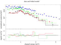
Given the evidence of a soft component with temperature in the range 1.3-1.5 keV and the surface brightness profile shown in Fig.3, we made an attempt (bearing in mind all the caveats of extracting a region comparable in size with the half energy width of the PSF) to extract a spectrum from a circular region of 10″ radius using as background a spectrum extracted from an annulus with bounding radii 15″-30″, both centered on the emission peak. The purpose of this attempt is to investigate the excess emission that might be associated with the presence of a cool corona. The use of the local background very close to the excess emission should subtract the hot thermal emission of the surrounding ICM thereby revealing the cooler emission of the corona. The spectrum of the inner 10″ is well fitted by a 1T model with $kT=1.46\pm 0.10$ keV. We find the same result if we simultaneously fit the two spectra and we take into account the spreading of the cooler X-rays from the very center due to the finite PSF by means of the cross-talk modification of the ARF generation software (e.g. Snowden et al. 2008). The spectrum with the best-fit model is shown in Fig.6 together with the pn spectrum of the 15″-30″ annulus to represent the hotter ICM in which the corona is embedded.

Figure 6: X-ray spectrum of the inner 10″ of the core of Abell 2028 A (having subtracted the emission coming from an annulus with bounding radii 15″-30″). Data from MOS1, MOS2, and pn are plotted in black, red, and green, respectively. The best-fit model obtained from a 1T fit and residuals are also shown. The pn spectrum taken from the 15″-30″ annulus is shown in blue for comparison.

Table 1: Results of the fits using single and multi-temperature models (see text for details of the models ) in different energy bands for the EPIC spectrum of the core (circle of 0.5′ radius) of A 2028 A.

Model/Band	$kT_{0}$	Z	Norm0	$kT_{1}$	Norm1	$\sigma_{T}$/width	$\alpha$	$\chi^{2}$/dof	Notes
(keV)	(keV)	($Z_{\odot}$)	($10^{-4}\rm{cm}^{-5}$)	(keV)	($10^{-4}\rm{cm}^{-5}$)	(keV)
1T 0.5-10	$2.95\pm 0.13$	$0.76\pm 0.14$	$1.70\pm 0.09$					243/168	Full spectrum
1T 0.5-6	$2.59\pm 0.10$	$0.55\pm 0.10$	$1.93\pm 0.09$					234/165	no Fe-K
1T 0.5-3	$1.99\pm 0.09$	$0.32^{+0.07}_{-0.05}$	$2.12\pm 0.09$					178/148	soft band Fe-L
2T 0.5-10	5.0 (fixed)	$0.53_{-0.11}^{+0.08}$	$1.20^{+0.11}_{-0.06}$	$1.48_{-0.15}^{+0.07}$	$0.65_{-0.18}^{+0.05}$			204/167
2T 0.5-10	4.0 (fixed)	$0.75_{-0.08}^{+0.13}$	$1.42^{+0.06}_{-0.03}$	$1.27_{-0.03}^{+0.07}$	$0.27_{-0.05}^{+0.02}$			204/167
GDEM 0.5-10	$3.92^{+0.16}_{-0.22}$	$1.18^{+0.28}_{-0.26}$	$1.69\pm 0.13$			$1.67^{+0.24}_{-0.22}$		202/167
PDEM1 0.5-10	$0.44\pm 0.08$	$1.55^{+0.45}_{-0.26}$	$1.36\pm 0.12$			$5.81^{+0.80}_{-0.71}$	$0.83^{+0.21}_{-0.18}$	197/166

¹ For PDEM $T_{0}$ corresponds to $T_{min}$ and the width to $T_{max}-T_{min}$

4.3 The spectrum of the large ASCA aperture

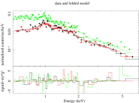
We extracted a spectrum from a circular region of 7′ centered on RA 15:09:29 DEC +07:34:20 (Horner 2001), which corresponds to the ASCA aperture (the white circle in Fig.4). We fitted a 1T model and multi-temperature models as done for the core of A2028 A. As expected given the wide range of temperatures revealed by the temperature map of Fig.4, the 1T model fails to accurately model the spectra of this ASCA aperture which include the bulk of emission of the two subclusters. The multi-temperature models also do not fit the spectra adequately. But significantly we do not see the large variations in metallicity among different models as seen in the case of the core of Abell 2028 A, and it is close to the average abundance in the various regions of this merging cluster as revealed by the two-dimensional map. There are enough counts to allow us to fit the spectrum just in the 2-10 keV energy band and to measure an abundance based just upon the Fe-K line. The results are consistent within the errors with all the previous determinations ($0.35\pm 0.05$ $Z_{\odot}$ obtained with a 1T fit in the 2-10 keV band, to be compared with the upper value of the range, $0.43\pm 0.03$ $Z_{\odot}$ obtained with the 1T and GDEM models in the 0.5-10 keV band, and the lower value, $0.33\pm 0.04$ $Z_{\odot}$ obtained with a 2T model in the 0.5-10 keV band).

Figure 7: Left panel: Exposure-corrected ASCA GIS image of Abell 2028. The regions inside the solid green lines (R=7^′) were extracted for the source spectrum analyzed in Baumgartner et al. (2005). Figure taken from http://asd.gsfc.nasa.gov/Donald.Horner/acc/html/ABELL_2028_83040050.html
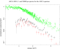
Right panel: Comparison of the X-ray spectra of the large ASCA aperture from the ASCA SIS 0 and 1 detectors (black and red, respectively) and from the EPIC pn (green).

         

Figure 8: Left panel: SDSS color image of the field of Abell 2028 Right panel: The RASS field of Abell 2028 highlighting in magenta the other members of the supercluster as Abell 2033 and Abell 2029.

5 Discussion

5.1 The inverse iron bias at work in Abell 2028

The XMM-Newton observation of Abell 2028 clearly shows its complex structure by revealing two merging subclusters, a more luminous SW component (A2028 A) and a less luminous NE component (A2028 B). Associated with the brightest central galaxy (BCG) of A2028 A, GIN 416, there is indication of a cool corona as suggested by the excess surface brightness profile and a cooler spectral component (Sun et al. 2007). The BCGs that able to retain their corona are usually associated with merging clusters, such as the first observed objects of this class, the BCGs in the Coma cluster (Vikhlinin et al. 2001a).

It is therefore clear that, within the beam of the ASCA region used to derive the abundances presented for A2028 in the work of Baumgartner et al. (2005), several components with different temperatures are present. Work by Mazzotta et al. (2004) and Vikhlinin (2006) pointed out how the temperature obtained by a fit with a single-temperature plasma model can be significantly different from commonly used definitions of average temperature like the emission-weighted temperature. However, as pointed out by Mazzotta et al. (2004), the spectrum of a multi-temperature model cannot be reproduced correctly by a single-temperature thermal model. On the other hand, a multi-temperature thermal emission may be well-fitted by a single-temperature model only because of the convolution with the instrument response, Poisson noise and background noise. Even more difficult to gauge is the concept of the spectroscopic-like abundances, i.e. the measured abundance using a single temperature fit to a multi-temperature spectrum with possible different abundances in different temperature components, because it depends strongly on the correct modeling of the temperature structure and on the limitations of current CCD detectors, which cannot spectrally separate emission from different components in a precise way. Besides the early discovery of the Fe bias (Buote 2000b), only recently work has been done to investigate this issue (Mazzotta et al. 2004; Balestra et al. 2007; Rasia et al. 2008).

In the work by Rasia et al. (2008), who analyzed six simulated galaxy clusters processed through an X-Ray Map Simulator (X-MAS, Gardini et al. 2004) that allows mock XMM-Newton MOS 1 and MOS 2 observations to be created, a systematic overestimate of iron for systems in the 2-3 keV range was found. By simulating a spectrum resulting from the combination of plasmas at 2 and 3 keV, they found fitted iron abundances higher with respect to the input value up to 40% in low S/N spectra (but still with 4500 counts). They also found the very interesting fact that the overestimate depends inversely on the number of counts, i.e. low S/N spectra have a greater bias. Projection and low resolution effects can create a complex temperature structure, averaging different temperatures in the same radial bin. Simionescu et al. (2009) give further support to this interpretation analyzing a 3′ aperture in the center of the cool core cluster Hydra A finding that a GDEM model is a better fit to the spectrum and that it returns a best-fit Fe abundance lower than the one obtained from a fit with a single-temperature model of the full spectral band. (Lower values are derived when fitting, in particular, just the soft band.)

The statistical quality of either the simulated spectra by Rasia et al. (2008) or the Hydra A spectra presented in Simionescu et al. (2009) are good, and in particular the Fe-K feature is clearly present. Many of the objects in the ASCA sample did not have sufficient signal-to-noise spectra for the Fe-K line emission to be present with the same statistical significance also because Baumgartner et al. (2005) did not include very bright clusters to not unduly bias the results of their stacking analysis. This is indeed the case for the XMM-Newton spectrum of the core of A 2028 A or the ASCA spectra of the 7′ large aperture of the cluster (see right panel of Fig.7). With the aid of the simulations presented in appendix A, we suggest that the inverse-Fe bias is mainly driven by the behavior of the the Fe-L complex strength which falls rapidly with increasing temperature above roughly 3 keV: in a multi-T spectrum where the average T is near 3 keV, but there are temperature components below and above 3 keV, most of the the Fe L emission of this multi-T spectrum comes from the lower-T components in the spectrum. However, when one fits a (wrong) single-T model, the single temperature will be sufficiently high that the Fe L lines will be weaker, and thus the model will have to compensate by increasing the Fe abundance above the true value. This is also shown by the central panel of Fig.5. That the Fe-K line is not necessary for the inverse iron bias to work can also be demonstrated by simulating 1T spectrum with the characteristics of the fit in the 0.5-3 keV band for the spectrum shown in Section 4.2, i.e. a single thermal spectrum with $kT=2.0$ keV and $Z=0.38$ $Z_{\odot}$. If we force the temperature in the model fit to be fixed at 3 keV (as in the case of a broad band fit where higher temperature components are present in the spectrum), the abundance will be biased high at a value of $Z=0.68$ $Z_{\odot}$. The thermal structure of a merging cluster is different from the very central regions of a cool core cluster and the main driver of the inverse Fe-bias in A2028 A is the cool component of the corona, which also justifies the simulations of Appendix A and fits with a 2T model, which seems a good physical description of a corona embedded in the hot intra-cluster gas. More complicated multi-temperature models, like the GDEM model, may provide on the contrary a more physical interpretation of the spectrum of the central regions of cool core clusters, as suggested by Simionescu et al. (2009).

The inverse-iron bias is, however, not present in the XMM-Newton EPIC spectra of the large 7′ aperture. The S/N of this spectrum is higher and the presence of a cool component is less important. This reinforces the fact already pointed out by Rasia et al. (2008) that the bias depends inversely on the number of counts present in the spectrum. It is beyond the scope of this paper to investigate the reasons for the anomalous abundances directly in the ASCA spectra but the presence of the inverse iron-bias in those low S/N spectra (obtained with a lower effective area instrument) is a reasonable suggestion. The XMM-Newton results for A2028 show that the abundances in this cluster are not anomalously high.

The presence of the direct iron bias (Buote 2000b) and of the inverse iron bias described in this paper show the danger of interpreting abundances measured with single-temperature fits to spectra extracted from large physical apertures (and of relatively low S/N), where there might be a great deal of temperature structure. This is particularly true for the combination of current telescopes and CCD detectors, which give a lot of weight to the soft energies and therefore to the shape of the Fe-L complex. Caution should be paid, for example, when interpreting global abundances measured in clusters out to a redshift of $z\sim$0.5 because the Fe-L shell of low-temperature components (down to $\sim$1 keV) is within fitting bandpasses with lower energy ends of 0.5-0.6 keV.

         

Figure 9: Left panel: Summed MOS and pn surface brightness profile across the cold front in the A1 sector of subcluster A shown in Fig.2, together with the best-fit model of a power law to describe the outer ICM and a $\beta$-model to describe the density inside the edge. Right panel: Same as the left panel for the cold front in sector B1 of subcluster B.

5.2 The dynamical state of Abell 2028

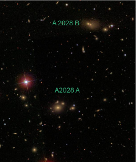
The X-ray morphology of the two subclusters associated with Abell 2028, with their tails and cold fronts, clearly suggests an off-axis merger as seen in various simulations (e.g. Ricker & Sarazin 2001). It is therefore interesting to look for other information about the dynamical state of the cluster at different wavelengths. Abell 2028 in the optical band is an elongated structure as shown by galaxy iso-density images (see Fig. 8 of Trevese et al. 1997) or by wavelet analysis (see the panels on scales of 750 kpc and 527 kpc of Fig.13 in Flin & Krywult 2006). On a scale of 258 kpc, Flin & Krywult (2006) detected substructures in the 2D galaxy distribution. These structures are coincident with the X-ray subclusters. The surface brightness peak of A 2028 A is coincident with the galaxy GIN 416, the BCG of the subcluster in the optical. The peak of A 2028 B is coincident with the pair of galaxies LEDA 140479 and 2MASX J15092098+0738225, which seem to be interacting (see the left panel of Fig.8). The velocities of these three galaxies are $cz=23148$ km s^-1, $cz=23011$ km s^-1, and $cz=23135$ km s^-1, suggesting a merger very close to the plane of the sky. The definitive confirmation of the presence of a corona has to wait for Chandra data with its better PSF; however further support is given by GIN 416 also being a radio source, NVSS 150928+073324, with $L_{\nu}=4.1\times 10^{23}$ W Hz^-1 (neglecting the small K-correction term), which is consistent with the idea that a radio active BCG should at least have a corona to be in such a state, because there is no large-scale cool core (Sun 2009).

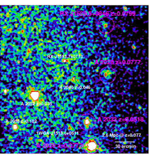
The galaxy distribution is elongated in the direction of the closest neighbor Abell 2033. Abell 2028 and Abell 2033, together with Abell 2029 and Abell 2066, form the super-cluster number 154 in the catalogue of Einasto et al. (2001). It is likely that another cluster can be added to the membership of the supercluster: the bright ROSAT source 1RXS J150935.9+084605 (Voges et al. 1999) is associated with a clustering of 25 SDSS galaxies, with measured spectroscopic redshifts, at the redshift of the supercluster (a Gaussian fit to the histogram of the galaxies with measured redshift gives $cz=23948$ km s^-1 corresponding to a redshift of z=0.0799, with a velocity dispersion $\sigma=574\pm 198$ km s^-1). The brightest galaxy in the field, SDSS J150936.33+084632.8, is a red elliptical whose photometric redshift measured by template fitting is $0.0788\pm 0.009$.

The subclusters of A 2028 are therefore merging to produce a more massive cluster belonging to this large-scale supercluster. If we coarsely indicate the direction of merging as indicated by the ”tails” of the two subclusters (and by the merging cold fronts perpendicular to them, see Markevitch & Vikhlinin 2007, and references therein), and the direction of the super-cluster as indicated by the four members in the right panel Fig.8, A2028 A and B are merging at $\sim 60^{\circ}$ direction with respect to the axis of the super-cluster. In order to bound in a quantitative way the motion of the two subclusters we determine the jump in gas density at the fronts, assuming that the gas density profile is described by the standard $\beta$ model $n=n_{0}\left[1+\left(r/r_{c}\right)^{2}\right]^{-3/2\beta}$ inside the cold front ($r>r_{cf}$ where $r_{cf}$ is the cold front radius) and by a power law $n=n_{1}\left(r\right)^{-\gamma}$ outside the cold front ($r>r_{cf}$). We then calculate the corresponding projected surface brightness. We fix the cold front radius at $r_{cf}=65$″ for the subclump A and $r_{cf}=65$″ for subclump B. We fit the outer part of the surface brightness profile (summing the MOS and pn profiles shown in Fig.2) to set the external component parameters, and we successively derive the best fit parameters of the innermost part. In Fig.9 we plot the surface brightness profiles with the best-fit models. We find a density discontinuity at the cold front in subcluster A of $n_{in}/n_{out}=3.11\pm 0.57$, which combined with the temperature values in the regions inside and outside the front (see Section4.1), leads to a pressure ratio $P_{in}/P_{out}=2.61\pm 0.53$. In subclump B, we find a density discontinuity at the cold front $n_{in}/n_{out}=5.86\pm 1.17$, which combined with the temperature values, leads to a pressure ratio $P_{in}/P_{out}=4.31\pm 0.98$. Following Vikhlinin et al. (2001b), these pressure ratios correspond to a Mach number ${\cal M}=1.19^{+0.15}_{-0.18}$ for subclump A and ${\cal M}=1.61^{+0.20}_{-0.22}$ for subclump B respectively.

6 Conclusions

We analyzed an XMM-Newton observation of Abell 2028, a $\sim 4$ keV cluster previously known with ASCA data to display anomalously high global abundances. The main results of our work can be summarized as follows:

• Abell 2028 is actually composed of two subclusters in the process of merging, along the axis of a supercluster. The evidence suggesting this interpretation is the cometary-like structure of the two subclusters with cold fronts at the leading edges of the two structures. The brightest galaxy of the main subcluster is likely hosting a cool corona;

• The abundance of the clusters, as derived from a temperature and abundance map, is consistent with the local abundance of more massive clusters. The abundances in every region chosen for spectral analysis show, with the appropriate temperature modeling, values in the range 0.3-0.5 $Z_{\odot}$, much lower than the previous ASCA global measurement of 0.77 $Z_{\odot}$ (in units of Anders & Grevesse 1989);

• We suggest that the inverse Fe-bias, i.e. the overestimate of iron abundance when fitting multi-temperature spectra with average spectroscopic temperature around 3 keV with a single temperature model, is likely the source of the high abundances in 3-4 keV local clusters as already discussed in the literature. We suggest that the behavior of the Fe-L shell lines explains the bias. The Fe-L complex strength falls rapidly with increasing temperature above roughly 3 keV: in a multi-T spectrum where the average T is near 3 keV, but there are temperature components below and above 3 keV, most of the the Fe L emission of this multi-T spectrum comes from the lower-T components in the spectrum. The best-fit single temperature will be high enough that the Fe L lines will be weaker, so the model will have to compensate by increasing the Fe abundance above the true value.

More definitive results will be obtained with our ongoing project of observing local clusters in the 3-4 keV range. More quantitative results for the dynamical state of A 2028 and for the cold fronts and corona detected in the XMM-Newton data will be possible with a dedicated Chandra follow-up.

Appendix A Analysis of simulated X-ray spectra

In this section we investigate the inverse Fe bias when fitting simulated multi-temperature models with a single-temperature plasma model. Following a well-established approach we assumed a double temperature model (2T) to simulate a plasma with substantial temperature structure (e.g. Buote 2000b; Balestra et al. 2007; Rasia et al. 2008). Even though it may be argued that a model with a more continuous distribution of emission measure could be more physically motivated (see for example the discussion for the core of Hydra A in Simionescu et al. 2009), it is difficult to disctinguish it with respect to a 2T model; this also seems to be realistic on physical grounds given the possible interpretation of a cool corona embedded in an ambient hotter plasma we put forward to explain the core of Abell 2028 A, which we used as a reference starting point for our simulations. We perform several simulations of spectra with different assumptions, as described in detail below, and explore the possible conditions that can potentially affect the distribution of best-fit values of $kT$ and, most important, of the metallicity $Z$.

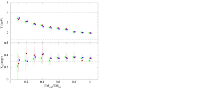
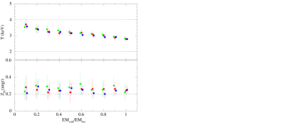
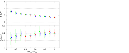
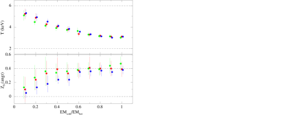
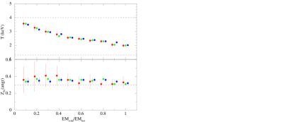
We performed a set of simulations of clusters with two temperature components (specified in Table 2) in the range relevant for the core of Abell 2028 A, i.e. 1.3-2 keV for the cold component and 4-6 keV for the hot component with an emission measure ratio (the normalization of the APEC model) ranging from 0.1 to 1.0 with steps of 0.1 between the two temperature components. The starting dominant component is listed as first, with an initial normalization (in XSPEC units) of $1.5\times 10^{-4}$. The total number of counts change as a function of the ratio $\rm{EM_{cold}/EM_{hot}}$ and ranges from $\sim$1100 counts and $\sim$2600 for MOS and pn in the 0.5-10 keV band in the simulations with $\rm{EM_{cold}/EM_{hot}}=0.1$ to $\sim$1800 and $\sim$4600 for MOS and pn in the simulations with $\rm{EM_{cold}/EM_{hot}}=1.0$. For each set of simulations, we performed 20 realizations and listed the results of the fits with a 1T model in the various table of results as median and mean absolute deviation from the median. We simulated spectra with the Galactic column density and redshift of A 2028 with an exposure time of 50 ks. We also investigated the distribution of best-fit abundances in the presence of a gradient in the abundance profile, with a higher abundance associated with the lower temperature component. We quote and plot the results separately for the three EPIC detectors to investigate the presence of effects arising by the difference in effective area.

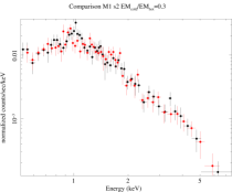
It can be seen by the plots of the results for the various simulations (from Fig. 10 to 15), which are also listed in Table 3, that, as the contribution of the low temperature component increases, the best-fit temperature of the single component model shifts to lower values. The distribution of the best fit abundance, either in cases with the same input abundance for the two components or in cases with an higher abundance in the lower temperature component, is always biased to higher values that a naive emission measure weighting would predict, up to $\sim 50$% of the median value compared to the input value in some cases. Even more striking is the large scatter in the distributions in particular for low values of the ratio $\rm{EM_{cold}/EM_{hot}}$ and for the MOS detectors, again pointing to the relevance of the Fe-L line in this bias: the fitting of the feature is key for the abundance determination, and Poisson noise is limiting for lower effective area instruments. Rather extreme values may occur: we show from example a MOS 1 s1 simulation when $\rm{EM_{cold}/EM_{hot}}=0.3$ (see Fig.16): the best-fit abundance is $0.72\pm 0.23$ $Z_{\odot}$ with a statistically good fit ($\chi^{2}/\rm{dof}<1$) with just a single temperature (we recall that the input abundance value for both components is 0.3 $Z_{\odot}$). It is instructive to plot this example together with another realization of the same model, with a best-fit abundance of $0.07^{+0.12}_{-0.07}$ $Z_{\odot}$, because it shows the importance of the fitting of the spectral region of the Fe-L lines (see Fig.17). In both cases the best fit temperatures are around $\sim 3$ keV. That the role played by the contribution of the Fe-K line is not relevant in the inverse Fe bias is also suggested by the simulation s6, where we only use a bremsstrahlung (i.e. the abundance was set to zero) for the hot component. Already for $\rm{EM_{cold}/EM_{hot}}=0.4$ the median best fit abundance is equal to the input abundance of the cold component.

The trends shown here do not change if one instead selects spectra with the same number counts as the ratio $\rm{EM_{cold}/EM_{hot}}$ increases. As an example we show the results in Fig.18 of the simulation s1 for MOS2 for three different number counts for all the $\rm{EM_{cold}/EM_{hot}}$ ratios, i.e. $1\times 10^{3}$, $5\times 10^{3}$ and $1\times 10^{4}$ counts in the 0.5-10 keV band.

Another result coming from the investigation of the simulations is that restricting the fitting energy band to just fit the shape of the Fe-L bump (for example in the 0.5-3 keV energy band) is no guarantee of recovering the abundance of the low-temperature component: the fitted continuum is too high because of the contribution of the high-temperature component and the abundance thus fitted is too low (see the green and blue pn spectra of Fig.6 for a visual representation).

Table 2: Input values for the spectral simulations of two temperature components as described in the Appendix

Bima	$kT_{inp}\mathrm{{}^{b}}$	$Z_{inp}\mathrm{{}^{c}}$
s1	4+1.3	0.3
s2	4+1.3	0.2+0.4
s3	4+2	0.2
s4	4+2	0.2+0.4
s5	5+2	0.2+0.4
s6	6+2	0.0+0.4

• ^a simulations identification number; ^b input temperature of the hot and cold component; ^c input iron abundance; ^c XSPEC fixed norm of the first temperature component ($\rm{cm}^{-5}$);

                                                        

Figure 10: Median of the best-fit temperature and abundance distribution as a function of the ratio of the cold and hot emission measure, for the simulation s1. The green dots refer to M1 results, the red dots to M2 and the blue dots to pn. The dashed lines refer to the input values of temperature and abundance for the two components. The error bars correspond to the mean absolute deviation.

                                                        

Figure 11: Same as in Fig.10 for the simulations s2. Note the two lines in the abundance panel which refer to the two different input abundances in the two components: the higher one (0.4 $Z_{\odot}$) in the cold component and the lower one (0.2 $Z_{\odot}$) in the hot component.

                                                        

Figure 12: Same as in Fig.10 for the simulations s3.

                                                        

Figure 13: Same as in Fig.10 for the simulations s4.

                                                        

Figure 14: Same as in Fig.10 for the simulations s5.

                                                        

Figure 15: Same as in Fig.10 for the simulations s6.

Figure 16: The MOS 1 spectrum and best fit 1T model with residuals for a realization of the simulation s1 with $\rm{EM_{cold}/EM_{hot}}=0.3$. The input model consists of two plasmas with $\rm{kT_{cold}}=1.3$ keV and $\rm{kT_{hot}}=4$ keV with an abundance of 0.3 $Z_{\odot}$ in both components, the single-temperature model best fit values are $\rm{kT}=3.02\pm 0.22$ keV and $\rm{Z}=0.72\pm 0.23$ $Z_{\odot}$.

Figure 17: Comparison of the MOS 1 spectra for two different realizations of the simulation s1 with $\rm{EM_{cold}/EM_{hot}}=0.3$: the black dots refer to the realization of Fig.16 and the red dots to a realization with best fit abundance of 0.07 $Z_{\odot}$.

                                                        

Figure 18: Median of the best-fit temperature and abundance distribution as a function of the ratio of the cold and hot emission measure, for the simulation s1 for the detector MOS2, with the same number counts for all the $\rm{EM_{cold}/EM_{hot}}$ ratios. The red dots refer to spectra with $1\times 10^{3}$ counts in the 0.5-10.0 keV band, the green ones to spectra with $5\times 10^{3}$ counts, and the blue to spectra with $1\times 10^{4}$ counts. The dashed lines refer to the input values of temperature and abundance for the two components. The error bars correspond to the mean absolute deviation.

Table 3: Fitted values with a 1T model in the 0.5-10 keV band for the three EPIC detectors of the simulations listed in Table 2.

	Ratio 0.1	0.2	0.3	0.4	0.5	0.6	0.7	0.8	0.9	1.0
					s1	M1
kT	$3.34\pm 0.22$	$3.11\pm 0.16$	$2.92\pm 0.17$	$2.74\pm 0.14$	$2.59\pm 0.14$	$2.48\pm 0.14$	$2.39\pm 0.15$	$2.09\pm 0.17$	$1.99\pm 0.13$	$1.98\pm 0.12$
Z	$0.26\pm 0.14$	$0.43\pm 0.12$	$0.40\pm 0.14$	$0.41\pm 0.15$	$0.35\pm 0.11$	$0.35\pm 0.08$	$0.36\pm 0.07$	$0.36\pm 0.10$	$0.31\pm 0.06$	$0.35\pm 0.07$
					s1	M2
kT	$3.42\pm 0.29$	$3.10\pm 0.27$	$2.88\pm 0.20$	$2.74\pm 0.17$	$2.53\pm 0.08$	$2.44\pm 0.11$	$2.32\pm 0.15$	$2.07\pm 0.15$	$2.05\pm 0.10$	$1.97\pm 0.07$
Z	$0.22\pm 0.23$	$0.31\pm 0.15$	$0.34\pm 0.13$	$0.35\pm 0.08$	$0.31\pm 0.07$	$0.36\pm 0.08$	$0.37\pm 0.07$	$0.37\pm 0.06$	$0.35\pm 0.07$	$0.31\pm 0.06$
					s1	pn
kT	$3.47\pm 0.16$	$3.15\pm 0.16$	$2.84\pm 0.14$	$2.59\pm 0.13$	$2.47\pm 0.09$	$2.37\pm 0.12$	$2.30\pm 0.14$	$2.08\pm 0.13$	$2.01\pm 0.07$	$1.96\pm 0.06$
Z	$0.32\pm 0.06$	$0.30\pm 0.07$	$0.37\pm 0.06$	$0.42\pm 0.07$	$0.35\pm 0.06$	$0.35\pm 0.06$	$0.35\pm 0.06$	$0.37\pm 0.05$	$0.36\pm 0.05$	$0.35\pm 0.04$
					s2	M1
kT	$3.51\pm 0.21$	$3.11\pm 0.24$	$2.84\pm 0.22$	$2.61\pm 0.17$	$2.43\pm 0.11$	$2.07\pm 0.14$	$2.02\pm 0.09$	$1.97\pm 0.06$	$1.90\pm 0.09$	$1.86\pm 0.13$
Z	$0.24\pm 0.13$	$0.33\pm 0.17$	$0.39\pm 0.11$	$0.40\pm 0.13$	$0.44\pm 0.08$	$0.35\pm 0.07$	$0.35\pm 0.07$	$0.33\pm 0.07$	$0.37\pm 0.04$	$0.33\pm 0.05$
					s2	M2
kT	$3.35\pm 0.24$	$3.00\pm 0.17$	$2.67\pm 0.22$	$2.50\pm 0.13$	$2.44\pm 0.17$	$2.24\pm 0.18$	$2.01\pm 0.10$	$1.98\pm 0.08$	$1.93\pm 0.08$	$1.89\pm 0.10$
Z	$0.32\pm 0.12$	$0.31\pm 0.09$	$0.32\pm 0.11$	$0.37\pm 0.08$	$0.47\pm 0.12$	$0.36\pm 0.08$	$0.35\pm 0.07$	$0.34\pm 0.06$	$0.34\pm 0.07$	$0.37\pm 0.07$
					s2	pn
kT	$3.36\pm 0.18$	$3.08\pm 0.16$	$2.65\pm 0.15$	$2.49\pm 0.08$	$2.40\pm 0.10$	$2.28\pm 0.17$	$2.02\pm 0.14$	$1.97\pm 0.06$	$1.89\pm 0.03$	$1.88\pm 0.03$
Z	$0.34\pm 0.11$	$0.36\pm 0.05$	$0.36\pm 0.04$	$0.36\pm 0.04$	$0.39\pm 0.05$	$0.36\pm 0.05$	$0.38\pm 0.05$	$0.36\pm 0.04$	$0.37\pm 0.04$	$0.37\pm 0.04$
					s3	M1
kT	$3.71\pm 0.30$	$3.43\pm 0.29$	$3.25\pm 0.26$	$3.15\pm 0.23$	$3.16\pm 0.22$	$3.19\pm 0.23$	$3.09\pm 0.17$	$3.01\pm 0.15$	$2.88\pm 0.16$	$2.79\pm 0.15$
Z	$0.28\pm 0.14$	$0.25\pm 0.10$	$0.22\pm 0.09$	$0.24\pm 0.09$	$0.22\pm 0.12$	$0.26\pm 0.07$	$0.26\pm 0.12$	$0.26\pm 0.10$	$0.26\pm 0.08$	$0.24\pm 0.07$
					s3	M2
kT	$3.55\pm 0.28$	$3.44\pm 0.21$	$3.40\pm 0.21$	$3.33\pm 0.22$	$3.24\pm 0.20$	$3.16\pm 0.18$	$3.12\pm 0.16$	$3.07\pm 0.13$	$2.93\pm 0.12$	$2.83\pm 0.15$
Z	$0.23\pm 0.11$	$0.30\pm 0.15$	$0.29\pm 0.14$	$0.27\pm 0.11$	$0.28\pm 0.09$	$0.32\pm 0.13$	$0.25\pm 0.09$	$0.25\pm 0.09$	$0.30\pm 0.11$	$0.22\pm 0.11$
					s3	pn
kT	$3.58\pm 0.18$	$3.39\pm 0.22$	$3.23\pm 0.16$	$3.24\pm 0.11$	$3.16\pm 0.11$	$3.05\pm 0.09$	$3.01\pm 0.12$	$2.91\pm 0.12$	$2.92\pm 0.13$	$2.79\pm 0.08$
Z	$0.21\pm 0.09$	$0.29\pm 0.09$	$0.25\pm 0.08$	$0.24\pm 0.10$	$0.27\pm 0.06$	$0.25\pm 0.06$	$0.21\pm 0.04$	$0.20\pm 0.05$	$0.24\pm 0.05$	$0.25\pm 0.05$
					s4	M1
kT	$3.58\pm 0.25$	$3.35\pm 0.23$	$3.25\pm 0.14$	$3.07\pm 0.18$	$3.05\pm 0.21$	$2.94\pm 0.14$	$2.93\pm 0.16$	$2.84\pm 0.11$	$2.82\pm 0.14$	$2.71\pm 0.15$
Z	$0.19\pm 0.16$	$0.34\pm 0.14$	$0.33\pm 0.15$	$0.31\pm 0.15$	$0.32\pm 0.08$	$0.37\pm 0.10$	$0.41\pm 0.11$	$0.42\pm 0.09$	$0.45\pm 0.08$	$0.41\pm 0.10$
					s4	M2
kT	$3.61\pm 0.23$	$3.36\pm 0.24$	$3.22\pm 0.17$	$3.14\pm 0.20$	$3.15\pm 0.16$	$3.07\pm 0.17$	$2.94\pm 0.14$	$2.86\pm 0.13$	$2.79\pm 0.10$	$2.74\pm 0.15$
Z	$0.25\pm 0.18$	$0.33\pm 0.19$	$0.35\pm 0.17$	$0.33\pm 0.14$	$0.34\pm 0.09$	$0.40\pm 0.07$	$0.45\pm 0.14$	$0.38\pm 0.12$	$0.40\pm 0.10$	$0.39\pm 0.08$
					s4	pn
kT	$3.54\pm 0.22$	$3.32\pm 0.11$	$3.20\pm 0.12$	$3.16\pm 0.14$	$3.09\pm 0.16$	$2.85\pm 0.10$	$2.90\pm 0.07$	$2.81\pm 0.09$	$2.72\pm 0.10$	$2.63\pm 0.08$
Z	$0.28\pm 0.09$	$0.32\pm 0.08$	$0.38\pm 0.07$	$0.38\pm 0.07$	$0.34\pm 0.08$	$0.35\pm 0.06$	$0.38\pm 0.06$	$0.37\pm 0.06$	$0.41\pm 0.07$	$0.40\pm 0.05$
					s5	M1
kT	$4.61\pm 0.47$	$3.92\pm 0.28$	$3.88\pm 0.27$	$3.59\pm 0.20$	$3.40\pm 0.18$	$3.22\pm 0.17$	$3.27\pm 0.15$	$3.11\pm 0.14$	$3.02\pm 0.15$	$3.00\pm 0.13$
Z	$0.26\pm 0.21$	$0.36\pm 0.18$	$0.32\pm 0.18$	$0.37\pm 0.16$	$0.44\pm 0.11$	$0.44\pm 0.11$	$0.44\pm 0.12$	$0.44\pm 0.10$	$0.46\pm 0.10$	$0.43\pm 0.12$
					s5	M2
kT	$4.53\pm 0.38$	$4.15\pm 0.25$	$3.83\pm 0.19$	$3.60\pm 0.21$	$3.36\pm 0.25$	$3.32\pm 0.23$	$3.32\pm 0.22$	$3.17\pm 0.17$	$3.15\pm 0.15$	$3.09\pm 0.16$
Z	$0.25\pm 0.18$	$0.42\pm 0.11$	$0.38\pm 0.14$	$0.42\pm 0.18$	$0.44\pm 0.11$	$0.49\pm 0.13$	$0.47\pm 0.14$	$0.41\pm 0.10$	$0.47\pm 0.12$	$0.48\pm 0.09$
					s5	pn
kT	$4.41\pm 0.31$	$4.02\pm 0.20$	$3.82\pm 0.18$	$3.63\pm 0.20$	$3.48\pm 0.16$	$3.34\pm 0.14$	$3.18\pm 0.11$	$3.13\pm 0.13$	$3.04\pm 0.05$	$2.93\pm 0.09$
Z	$0.27\pm 0.13$	$0.36\pm 0.08$	$0.37\pm 0.08$	$0.32\pm 0.08$	$0.43\pm 0.08$	$0.42\pm 0.07$	$0.41\pm 0.09$	$0.42\pm 0.08$	$0.47\pm 0.08$	$0.43\pm 0.05$
					s6	M1
kT	$5.23\pm 0.48$	$4.87\pm 0.42$	$4.26\pm 0.29$	$4.05\pm 0.24$	$3.78\pm 0.29$	$3.36\pm 0.23$	$3.30\pm 0.18$	$3.20\pm 0.18$	$3.12\pm 0.18$	$3.12\pm 0.16$
Z	$0.10\pm 0.18$	$0.24\pm 0.15$	$0.33\pm 0.18$	$0.39\pm 0.17$	$0.33\pm 0.13$	$0.37\pm 0.11$	$0.41\pm 0.16$	$0.40\pm 0.09$	$0.40\pm 0.11$	$0.39\pm 0.11$
					s6	M2
kT	$5.09\pm 0.47$	$4.47\pm 0.28$	$4.13\pm 0.30$	$3.91\pm 0.27$	$3.74\pm 0.22$	$3.64\pm 0.30$	$3.30\pm 0.23$	$3.16\pm 0.18$	$3.14\pm 0.20$	$3.02\pm 0.16$
Z	$0.13\pm 0.16$	$0.27\pm 0.18$	$0.36\pm 0.21$	$0.34\pm 0.13$	$0.36\pm 0.13$	$0.38\pm 0.10$	$0.40\pm 0.09$	$0.39\pm 0.09$	$0.44\pm 0.11$	$0.47\pm 0.10$
					s6	pn
kT	$5.30\pm 0.34$	$4.92\pm 0.33$	$4.51\pm 0.25$	$4.11\pm 0.21$	$3.83\pm 0.26$	$3.57\pm 0.17$	$3.33\pm 0.15$	$3.14\pm 0.09$	$3.02\pm 0.13$	$3.11\pm 0.14$
Z	$0.05\pm 0.07$	$0.13\pm 0.10$	$0.18\pm 0.12$	$0.24\pm 0.06$	$0.24\pm 0.09$	$0.35\pm 0.07$	$0.36\pm 0.07$	$0.37\pm 0.08$	$0.35\pm 0.05$	$0.38\pm 0.06$

References

- Anders & Grevesse (1989) Anders, E. & Grevesse, N. 1989, Geochim. Cosmochim. Acta., 53, 197
- Arimoto et al. (1997) Arimoto, N., Matsushita, K., Ishimaru, Y., Ohashi, T., & Renzini, A. 1997, ApJ, 477, 128
- Balestra et al. (2007) Balestra, I., Tozzi, P., Ettori, S., et al. 2007, A&A, 462, 429
- Baumgartner et al. (2005) Baumgartner, W. H., Loewenstein, M., Horner, D. J., & Mushotzky, R. F. 2005, ApJ, 620, 680
- Borgani et al. (2008) Borgani, S., Fabjan, D., Tornatore, L., et al. 2008, Space Science Reviews, 134, 379
- Buote (2000a) Buote, D. A. 2000a, ApJ, 539, 172
- Buote (2000b) Buote, D. A. 2000b, MNRAS, 311, 176
- Buote & Fabian (1998) Buote, D. A. & Fabian, A. C. 1998, MNRAS, 296, 977
- Buote et al. (2003a) Buote, D. A., Lewis, A. D., Brighenti, F., & Mathews, W. G. 2003a, ApJ, 594, 741
- Buote et al. (2003b) Buote, D. A., Lewis, A. D., Brighenti, F., & Mathews, W. G. 2003b, ApJ, 595, 151
- Davis et al. (1999) Davis, D. S., Mulchaey, J. S., & Mushotzky, R. F. 1999, ApJ, 511, 34
- De Grandi & Molendi (2001) De Grandi, S. & Molendi, S. 2001, ApJ, 551, 153
- De Luca & Molendi (2004) De Luca, A. & Molendi, S. 2004, A&A, 419, 837
- Einasto et al. (2001) Einasto, M., Einasto, J., Tago, E., Müller, V., & Andernach, H. 2001, AJ, 122, 2222
- Flin & Krywult (2006) Flin, P. & Krywult, J. 2006, A&A, 450, 9
- Fujimoto et al. (2007) Fujimoto, R., Mitsuda, K., Mccammon, D., et al. 2007, PASJ, 59, 133
- Gardini et al. (2004) Gardini, A., Rasia, E., Mazzotta, P., et al. 2004, MNRAS, 351, 505
- Gastaldello et al. (2007) Gastaldello, F., Buote, D. A., Humphrey, P. J., et al. 2007, ApJ, 662, 923
- Gonzalez et al. (2007) Gonzalez, A. H., Zaritsky, D., & Zabludoff, A. I. 2007, ApJ, 666, 147
- Horner (2001) Horner, D. J. 2001, PhD thesis, University of Maryland College Park
- Humphrey & Buote (2006) Humphrey, P. J. & Buote, D. A. 2006, ApJ, 639, 136
- Kalberla et al. (2005) Kalberla, P. M. W., Burton, W. B., Hartmann, D., et al. 2005, A&A, 440, 775
- Kuntz & Snowden (2008) Kuntz, K. D. & Snowden, S. L. 2008, A&A, 478, 575
- Liedahl et al. (1995) Liedahl, D. A., Osterheld, A. L., & Goldstein, W. H. 1995, ApJ, 438, L115
- Lin et al. (2003) Lin, Y.-T., Mohr, J. J., & Stanford, S. A. 2003, ApJ, 591, 749
- Markevitch & Vikhlinin (2007) Markevitch, M. & Vikhlinin, A. 2007, Phys. Rep, 443, 1
- Matsumoto et al. (1997) Matsumoto, H., Koyama, K., Awaki, H., et al. 1997, ApJ, 482, 133
- Matsushita et al. (2007) Matsushita, K., Fukazawa, Y., Hughes, J. P., et al. 2007, PASJ, 59, 327
- Mazzotta et al. (2004) Mazzotta, P., Rasia, E., Moscardini, L., & Tormen, G. 2004, MNRAS, 354, 10
- Mewe et al. (1985) Mewe, R., Gronenschild, E. H. B. M., & van den Oord, G. H. J. 1985, A&AS, 62, 197
- Molendi & Gastaldello (2001) Molendi, S. & Gastaldello, F. 2001, A&A, 375, L14
- Nevalainen et al. (2005) Nevalainen, J., Markevitch, M., & Lumb, D. 2005, ApJ, 629, 172
- Pradas & Kerp (2005) Pradas, J. & Kerp, J. 2005, A&A, 443, 721
- Pratt & Arnaud (2002) Pratt, G. W. & Arnaud, M. 2002, A&A, 394, 375
- Protassov et al. (2002) Protassov, R., van Dyk, D. A., Connors, A., Kashyap, V. L., & Siemiginowska, A. 2002, ApJ, 571, 545
- Rasia et al. (2008) Rasia, E., Mazzotta, P., Bourdin, H., et al. 2008, ApJ, 674, 728
- Renzini (1997) Renzini, A. 1997, ApJ, 488, 35
- Renzini (2004) Renzini, A. 2004, in Clusters of Galaxies: Probes of Cosmological Structure and Galaxy Evolution, ed. J. S. Mulchaey, A. Dressler, & A. Oemler, 260–+
- Ricker & Sarazin (2001) Ricker, P. M. & Sarazin, C. L. 2001, ApJ, 561, 621
- Saxton & Siddiqui (2002) Saxton, R. D. & Siddiqui, H. 2002, XMM-SOC-PS-TN-43
- Schindler & Diaferio (2008) Schindler, S. & Diaferio, A. 2008, Space Science Reviews, 134, 363
- Simionescu et al. (2009) Simionescu, A., Werner, N., Böhringer, H., et al. 2009, A&A, 493, 409
- Smith et al. (2001) Smith, R. K., Brickhouse, N. S., Liedahl, D. A., & Raymond, J. C. 2001, ApJ, 556, L91
- Snowden et al. (2004) Snowden, S. L., Collier, M. R., & Kuntz, K. D. 2004, ApJ, 610, 1182
- Snowden et al. (2008) Snowden, S. L., Mushotzky, R. F., Kuntz, K. D., & Davis, D. S. 2008, A&A, 478, 615
- Struble & Rood (1999) Struble, M. F. & Rood, H. J. 1999, ApJS, 125, 35
- Sun (2009) Sun, M. 2009, ApJ, 704, 1586
- Sun et al. (2007) Sun, M., Jones, C., Forman, W., et al. 2007, ApJ, 657, 197
- Trevese et al. (1997) Trevese, D., Cirimele, G., Cenci, A., et al. 1997, A&AS, 125, 459
- Vikhlinin (2006) Vikhlinin, A. 2006, ApJ, 640, 710
- Vikhlinin et al. (2001a) Vikhlinin, A., Markevitch, M., Forman, W., & Jones, C. 2001a, ApJ, 555, L87
- Vikhlinin et al. (2001b) Vikhlinin, A., Markevitch, M., & Murray, S. S. 2001b, ApJ, 551, 160
- Vikhlinin et al. (2005) Vikhlinin, A., Markevitch, M., Murray, S. S., et al. 2005, ApJ, 628, 655
- Voges et al. (1999) Voges, W., Aschenbach, B., Boller, T., et al. 1999, A&A, 349, 389
- Werner et al. (2006) Werner, N., de Plaa, J., Kaastra, J. S., et al. 2006, A&A, 449, 475
- Werner et al. (2008) Werner, N., Durret, F., Ohashi, T., Schindler, S., & Wiersma, R. P. C. 2008, Space Science Reviews, 134, 337
- Yoshino et al. (2009) Yoshino, T., Mitsuda, K., Yamasaki, N. Y., et al. 2009, PASJ, 61, 805