Empirical optical k-corrections for redshifts 0.7
Abstract
The Smithsonian Hectospec Lensing Survey (SHELS) is a magnitude-limited spectroscopically complete survey for covering 4 □°. SHELS provides a large sample (15,513) of flux-calibrated spectra. The wavelength range covered by the spectra allows empirical determination of k-corrections for the and bands from to and 0.33, respectively, based on large samples of spectra. We approximate the k-corrections using only two parameters in a standard way: and redshift, . We use rather than the standard observed galaxy color because is a redshift-independent tracer of the stellar population of the galaxy. Our approximations for the k-corrections using are as good as those based on observed galaxy color ( of the scatter is mag). The approximations for the k-corrections are available in an online calculator. Our results agree with previously determined analytical approximations from single stellar population (SSP) models fitted to multiband optical and near-infrared photometry for galaxies with a known redshift. Galaxies with the smallest —the galaxies with the youngest stellar populations—are always attenuated and/or contain contributions from older stellar populations. We use simple single SSP fits to the SHELS spectra to study the influence of emission lines on the k-correction. The effects of emission lines can be ignored for rest-frame equivalent widths (REWs) Å depending on required photometric accuracy. We also provide analytic approximations to the k-corrections determined from our model fits for as a function of redshift and for and ( of the scatter is typically mag, the root-mean-square typically mag). Again, the approximations using are as good those based on a suitably chosen observed galaxy color. We provide all analytical approximations in an online calculator.
1 Introduction
The expansion of the Universe shifts the spectrum of galaxies redward with respect to the observer. Observing galaxies at different cosmological distances in a fixed bandpass thus leads to a different absolute magnitude in the bandpass after correcting for luminosity distance. To compare the photometric properties of galaxies at different redshifts, one needs to bring the photometry of these galaxies onto a common system. The correction that places the absolute magnitude on a common system is the k-correction (after Hubble, 1936). The k-correction is usually defined with respect to photometric observations of a galaxy in its rest frame, i.e., .111To remove large systematic uncertainties from the k-correction, sometimes the choice for a non-rest frame is made (e.g., Blanton & Roweis, 2007). Accurate k-corrections have increasing importance as cosmological observations become more precise. Here, we provide k-corrections based on —a spectroscopic indicator that is a measurement of the strength of the 4000 Å, or Balmer break—and redshift accurate to 0.1 mag with negligible systematic errors.
The k-correction is the correction in magnitudes between the observed magnitude in the filter and true rest-frame absolute magnitude in the filter at distance modulus (e.g., Hogg et al., 2002; Blanton & Roweis, 2007):
| (1) |
where and is the luminosity distance. We consider the case where filter is equal to filter .
To determine the k-correction of a galaxy, one approach is to model the spectral energy distribution (SED) of the galaxy over the wavelengths necessary to determine the k-correction. The quality of the k-correction is then limited by the adequacy of the models; when using photometric SEDs rather than spectra, the quality is limited by the number (and width) of the photometric bands used. A second approach is direct determination of the k-correction from the observed spectrum of the galaxy. Using observed spectra for calculating the k-corrections removes the need for model assumptions and empirically addresses all of the physics required to determine the SED of a galaxy.
Recently, Chilingarian et al. (2010, hereafter CMZ10) approximated the k-corrections for nine optical and near-infrared filters () with analytical functions of only two parameters: redshift and observed galaxy color. They used the measured redshift to fit a set of SSP models based on pegase.2 (Fioc & Rocca-Volmerange, 1997) to the photometry in the nine bands. From the fitted models, they derived k-corrections for the filter set.
Here, we discuss k-corrections determined directly from spectra from the Smithsonian Hectospec Lensing Survey. SHELS is a spectroscopic survey covering 4 □° on the sky to a limiting magnitude (Geller et al., 2005, Kurtz et al. 2011, in preparation). Instead of observed galaxy color, we use the of the galaxy together with redshift to parametrize the k-correction.
is the ratio of average flux red- and blueward of the so-called 4000 Å break, or Balmer break
| (2) |
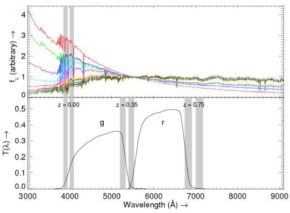
where is the rest-frame flux density of the galaxy and each wavelength is the rest-frame wavelength. We indicate the regions where we measure (Fig. 1) with respect to the Charlot & Bruzual (private communication 2010) (hereafter CB07) models at three different redshifts. We also show the and band throughput curves from the SDSS Web site222See http://www.sdss.org/dr7/instruments/imager/index.html..
The wavelength range covered by the Hectospec spectra determines the choice of filters for which we can determine the k-corrections. We can determine k-corrections only for bandpasses that satisfy the “Goldilocks principle”: if the bandpass is too blue, we can determine the rest-frame magnitude, not the observed-frame magnitude; if the bandpass is too red, we can determine the observed-frame magnitude, not the rest-frame magnitude. We need both observed- and rest-frame magnitudes to determine the k-correction. Two filters that satisfy this principle are the SDSS and bands. We derive these k-corrections (and analytic approximations) in Section 4.
We discuss the SHELS spectroscopic data in Section 2. In Section 3, we describe the methods used to calculate the k-corrections, the sample selection, and the use of as an indicator for galaxy type. We present the k-corrections in Section 4. We compare our results with our SSP fits based on CB07 to the previous work of CMZ10 in Section 5. We discuss the accuracy of our in Section 6. In Section 7 we discuss the impact of emission lines on the k-correction. We provide the k-corrections for SDSS bandpasses and the Johnson-Cousins derived from our model fits to the spectra in Section 8. We summarize our results in Section 9.
Throughout this article we assume a flat universe with km s-1 Mpc-1, , and . All quoted magnitudes are on the AB-system (Oke & Gunn, 1983).
2 The data
Here, we describe the observations of SHELS. We first describe the imaging and spectroscopic data. We then address the effects of fixed solid-angle aperture sizes on our measurements. We conclude with the selection criteria of our sample of spectra from which we determine our k-corrections.
2.1 The observations
We draw our data from an expanded SHELS catalog (cf. Fabricant et al., 2005; Geller et al., 2005; Kurtz et al., 2007; Geller et al., 2010; Westra et al., 2010; Woods et al., 2010, who use a previous version of the catalog). The main differences with the prior catalog are: (1) we select fainter targets, because the survey now reaches , instead of ; (2) we have more redshifts available (15,513 unique redshifts compared with 11,447 previously); and (3) we have updated the photometry. We next summarize the galaxy catalog construction. We discuss the details in a forthcoming article (Kurtz et al. 2010, in preparation).
We constructed the SHELS galaxy catalog from the -band source list for the F2 field of the Deep Lens Survey (Wittman et al., 2002, 2006). The imaging of F2 is extremely deep; the imaging has a 1 surface brightness limit of 28.7 mag/ in . The effective exposure time with the MOSAIC I imager (Muller et al., 1998) on the Kitt Peak National Observatory Mayall 4 m telescope is about 14,500 s. All exposures are observed in less than seeing between 1999 November and 2004 November. Wittman et al. (2006) describe the reduction pipeline. The 4.2 □° F2 field is centered at and . We exclude regions around bright stars ( 5 % of the total survey), resulting in an effective area of 4.0 □°. We use surface brightness and magnitude in combination with information from the latest SDSS data release (DR7; Abazajian et al., 2009) to separate stars from galaxies. This selection removes some active galactic nuclei (AGNs). The final catalog contains 20,116 galaxies with a total -band magnitude of 21.0.
We acquired spectra for the galaxies with the Hectospec fiber-fed spectrograph (Fabricant et al., 1998, 2005) on the MMT on various nights during the period from 2004 April 13 through 2009 December 15. The Hectospec observation planning software (Roll et al., 1998) enables efficient acquisition of a magnitude-limited sample.
The SHELS spectra cover the wavelength range of Å with a resolution of 6 Å. Exposure times ranged from 0.75 hr to 2 hr for the lowest surface brightness objects in the survey. We reduced the data with the standard Hectospec pipeline (Mink et al., 2007) and derived redshifts with RVSAO (Kurtz & Mink, 1998) with templates constructed for this purpose (Fabricant et al., 2005). The 1468 unique pairs of repeat observations imply a mean internal error of 56 km s-1 for absorption-line objects and 21 km s-1 for emission-line objects (see also Fabricant et al., 2005).
We photometrically calibrate the spectra by scaling the flux density obtained by the 15 diameter fiber to the total band. Fabricant et al. (2008) describe the technique used for the Hectospec spectra in detail. We can photometrically calibrate the data from this fiber-fed spectrograph because it has a particularly stable instrument response. This method assumes that the inner 15 of a galaxy is representative for the entire galaxy. See Section 2.2 for a more detailed discussion of aperture effects.
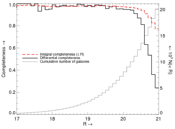
SHELS includes 20,116 galaxies to the limiting apparent magnitude. The integral completeness of the redshift survey is 96.5 %, 93.8 %, and 77.3 % to , 20.6, and 21.0, respectively. Figure 2 shows the integral and differential completeness of SHELS as a function of total magnitude.
2.2 Aperture effects
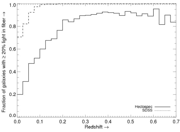
The Hectospec fibers subtend 15 on the sky, sampling only the inner region of a galaxy. For a given galaxy, the fraction of light contained in a fixed angular aperture increases with increasing redshift. Kewley et al. (2005) study the influence of fixed aperture size on the determination of star formation rate, metallicity, and attenuation in a galaxy. Their conclusion is that when the aperture contains more than 20 % of the light, the central region is a good representation of the entire galaxy. Like Woods et al. (2010), we use the -band data to compute the fraction of galaxies where at least 20 % of the light is contained in the Hectospec fiber aperture. The majority of our galaxies fulfill this requirement (Fig. 3).
Fabricant et al. (2005) find no difference between the determined from the SDSS spectra and the from the Hectospec spectra (their Fig. 12). The median redshift of the SDSS is : at this redshift, at least 20 % of the light of a galaxy is captured in an SDSS fiber (Fig. 3).
Galaxies with less than 20 % of their light captured by the Hectospec fibers are predominantly at low redshifts. A small difference in color between the nuclear region and the entire galaxy only leads to a small uncertainty in the k-correction, due to the low redshift; at low redshifts, the 4000 Å-break has not yet moved out of the filter (Fig. 1), resulting only in small k-corrections.
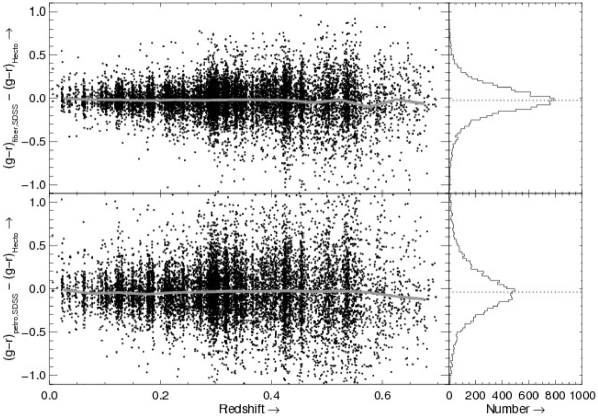
We also assume that the galaxy color measured in a fixed aperture on the sky is a good representation of the galaxy. The color obviously varies with aperture in a galaxy with a bulge and an extended disk. To investigate the effect of our simplifying assumption, we compare for three different apertures. Figure 4 shows the comparison between derived from the SDSS fiber spectra covering the inner 3″ of a galaxy and from the Hectospec fiber spectra subtending the inner 15 of a galaxy. The figure also shows a comparison between the from the SDSS Petrosian magnitudes, which include nearly all the galaxy light (Blanton et al., 2001; Yasuda et al., 2001), and determined from the Hectospec fiber spectra. The larger scatter in the lower diagram reflects the large uncertainties in the Petrosian magnitudes.
We find no significant trend for within different apertures as a function of redshift. There is a slight offset (median of and ), smaller than the median uncertainty for each of the individual SDSS and magnitudes. This offset occurs because the outer parts of a galaxy is bluer than the bulge (see also Kauffmann et al., 2003). The effect on the determination of the k-corrections is negligible.
We conclude that and determined from a Hectospec spectrum are reasonable representations of the and obtained from a spectrum that covers the entire galaxy.
2.3 Sample selection
To derive the best k-corrections, we select a subsample of spectra from the sample of 15,513 galaxies with unique redshifts. We retain the spectra of galaxies satisfying all of the following criteria:
-
•
The spectrum was observed after 2004 October 30. Until this date, the atmospheric dispersion compensation prisms of Hectospec rotated in the wrong direction (Fabricant et al., 2008). The spectra before this date have improper spectrophotometric calibration. However, the redshifts for these galaxies are not affected.
-
•
The model fit (Section 3.2) succeeds and the reduced of the fit is less than 10. This restriction mostly removes strong broad lined AGN, very strong emission-line galaxies, and spectra with bad sky-subtraction.
-
•
The median of the signal-to-noise ratio (S/N) per pixel for ten regions free of night-sky emission lines exceeds 2.
-
•
The redshift of the galaxy allows the determination of both the observed- and rest-frame magnitude.
After applying these selection criteria, we have samples of 11,707 and 5993 spectra to calculate the k-corrections for and , respectively.
3 Method
Here, we describe the method for determining the k-corrections from our spectra. We first outline the formulae used to derive the magnitudes. We also describe the fitting of SSP models to our spectra. Finally, we discuss the advantages of using rather than observed color as an identifying characteristic of a galaxy.
3.1 Synthetic magnitudes
We use flux-calibrated spectra (and SSP model fits; Section 3.2) to calculate the observed- and rest-frame magnitudes required for the k-corrections. We compute the effective flux-density from the observed spectrum for a particular bandpass
| (3) |
where is the flux density as a function of wavelength in Å, i.e. the flux-calibrated spectrum in units of erg s-1 cm-2 Å-1, and is the filter transmission curve per photon with wavelength.333Blanton & Roweis (2007) note that many authors give the transmission curve as the contribution to the detector signal per unit of energy (), rather than per photon (). They relate to each other as . However, accidentally using as has a very small impact (at the very worst 0.07 mag, and typically 0.02 mag or less for this survey).
We convert into the effective flux-density as a function of frequency :
| (4) |
where is in erg s-1 cm-2 Hz-1, in erg s-1 cm-2 Å-1, and is in angstrom. We calculate the artificial magnitude as
| (5) |
where 3631 Jy is the zeropoint of the AB-magnitude system (Oke & Gunn, 1983).
Throughout this article, unless otherwise noted, we determine the k-corrections from synthetic observer and rest-frame magnitudes. We obtain the observed colors of the galaxies from the SDSS fiber magnitudes; when these magnitudes are unavailable, we determine them from our synthetic magnitudes.
3.2 Model fitting
We use the method of Tremonti et al. (2004) to fit a linear combination of 10 SSP models to each spectrum. The SSP models are from CB07. These models include an improved treatment of the thermal pulse asymptotic giant branch phase with respect to the models of Bruzual & Charlot (2003) (see Bruzual, 2006, for more details). The 10 different ages for the populations are 0.005, 0.025, 0.1, 0.25, 0.5, 1, 1.4, 2.5, 5, and 10 Gyr. The models have solar metallicity. Figure 1 shows the individual model spectra normalized to 1 at 5500 Å together with the SDSS and bands. We use the Calzetti et al. (2000) extinction law rather than the Charlot & Fall (2000) extinction law used by Tremonti et al. (2004), but the difference is small (10 % at the extremes of the wavelength range 4000 Å – 10,000 Å).
We fit the models to the wavelength region between 4000 and 8500 Å; we use the fits to determine (Section 3.3) and remove residuals of night-sky features in our spectra (Section 4). The cut at the blue end of the spectrum is due to the uncertain calibration of Hectospec in that region. Beyond 8500 Å light emitted from the home sensors in the fiber positioner of the spectrograph affects the spectrum. Because this effect is additive, we cannot remove this problem.
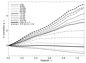
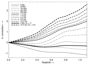
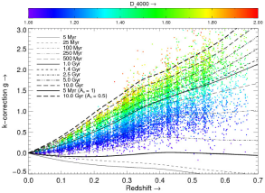
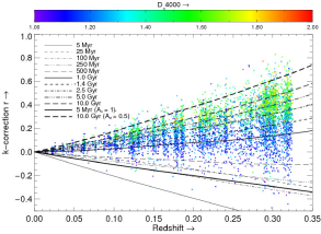
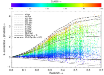
Figure 5 shows the predicted k-corrections as a function of redshift for each model without attenuation. We include two models with attenuation to show its effect on the k-correction. We apply a typical reddening for star-forming galaxies to the model with the youngest stellar population () and a reasonably extreme reddening for early-type galaxies to the model with the oldest stellar population (). Figure 5 shows approximately the full range of expected k-corrections modulo the effects of emission lines (see Section 7).
3.3 versus color
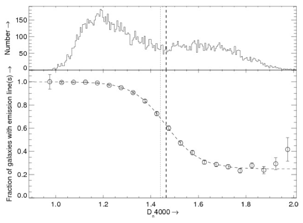
We use as a measure of galaxy type because it is an indicator of the age of the stellar population (see Table 1; Balogh et al., 1999; Bruzual, 1983). Woods et al. (2010) examine the fraction of galaxies with emission lines as a function of (they remove AGNs from their sample). Galaxies with a low invariably show emission lines; the fraction of galaxies with emission lines decreases rapidly with increasing . Kauffmann et al. (2003) show a very clear relation between and H (a measure for the REW of H). Kauffmann et al. also show clear evolution in both and H after an instantaneous burst of star formation as a function of time.
Figure 6 shows the distribution of for our sample, along with the fraction of galaxies with at least one emission line. We classify a galaxy as having an emission line when the absorption-corrected REW is at least 5 Å for any of the following emission lines: H, H, [O iii] 4959, [O iii] 5007, or [Oii] 3726,3728. Our distribution is double-peaked with a local minimum around (thick dashed line), very close to the Woods et al. (2010) value of 1.44 (dotted line).
Almost all galaxies with a low () show emission lines indicating an episode of active (or very recent, roughly less than 10 Myr ago) star formation, yielding a spectrum dominated by young, hot stars. The fraction of galaxies with emission lines gradually decreases with increasing . For galaxies with a large 4000 Å-break, an old stellar population dominates the spectrum. In our sample, toward the highest the number of galaxies with emission lines increases slightly because of the presence of AGNs.
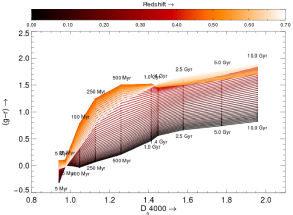
An advantage of over observed color is that is insensitive to reddening; is measured over a small wavelength range (see Fig. 1). In addition to the for the 10 SSP, we show the for two of these models with some attenuation in Table 1. Attenuation affects only minimally. Furthermore, the small wavelength range needed to calculate allows the use of uncalibrated spectra, provided that the sensitivity of the spectrograph does not vary significantly over the relevant wavelengths.
Another advantage of is—by its definition—independence of redshift; the observed color of a galaxy changes dramatically with redshift. At different redshifts, the bandpasses probe different parts of the spectrum. Thus, the k-corrections are not (necessarily) equal for different filters. Consider, for example, the 4000 Å break, a large-scale feature (in wavelength) in the galaxy spectrum where the flux can change significantly. The 4000 Å break is just in the band at , leaves it around and enters the band, and leaves the band at (see Fig. 1).444Similarly, the Lyman break causes drastic changes in galaxy colors as a function of redshift, which is a property employed in selecting higher redshift galaxies with the drop-out technique (Steidel et al., 1995).
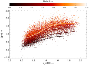
Figure 7 shows observed as function of for both the separate SSP models and the individual galaxies. We indicate the median color of the galaxies binned by redshift as function of . Toward higher , becomes less sensitive than to the age of the stellar population of a galaxy. Furthermore, the models show that is not a monotonic function of redshift; is redshift-independent.
A spectrum of a galaxy adequate to determine its redshift (a necessary quantity to calculate the k-correction) usually straightforwardly provides the of that galaxy. The is more robust for galaxies where older stellar populations dominate the spectrum; the redshift is then usually determined from the Ca H+K lines.
We use the determined from our model fits. This approach allows us to determine the more accurately for lower S/N spectra, because we use almost the entire wavelength range of the spectrum to constrain the model fit; the fits reflect the noise over the entire spectrum rather than the noise in a small portion of the spectrum around 4000 Å.
4 Empirically determined k-corrections
Here, we derive the empirically determined k-corrections from our spectra and from the model fits to the spectra as a function of redshift and . We also provide an online calculator.555See http://tdc-www.cfa.harvard.edu/instruments/hectospec/progs/EOK/.
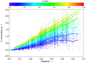
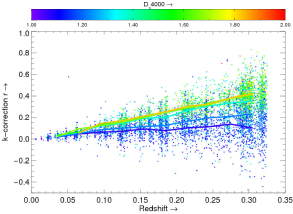
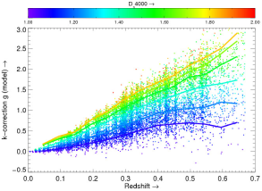
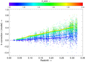
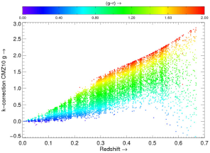
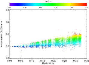
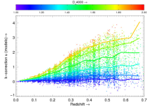
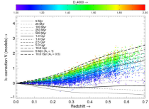
To minimize the impact of large residuals of night-sky features in our spectra, we replace the observed spectrum around these wavelengths with the model fit. We follow the same procedure for observed wavelengths blueward of 4000 Å and redward of 8500 Å because of the uncertainties in the flux calibration of our spectra. Using the definition of the k-correction (eq. [1]) and the prescription for determining artificial magnitudes from our spectra (Section 3.1), we determine the k-corrections from both our spectra and the model fits. Figure 8 gives the resulting k-corrections for the and band. Each galaxy is color-coded by its .
To use these results for other observed galaxies, we approximate these results with a two-dimensional surface in a fashion similar to that of CMZ10. We use a minimization to fit a two-dimensional surface to our data. We describe the fitting method in detail in the Appendix. We give a short summary here. To derive the fit, we use the redshift, , and determined k-correction (respectively, , , and in eq. [A2] and eq. [A3]) for all galaxies satisfying the sample selection of Section 2.3 to derive the fit. We choose the maximum polynomial orders for the redshift and ( and in eq. [A1], respectively) to be the lowest orders that do not show an obvious pattern in the residuals after fitting. If we use too many orders, the fit provides inaccurate results for the highest redshifts or extreme values, because the number of galaxies constraining the fit is limited. At the fit is constrained by the definition that the k-correction is zero (Section 1). For our fits, and are appropriate.
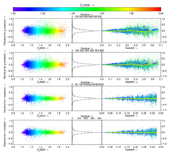
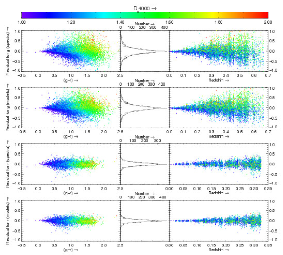
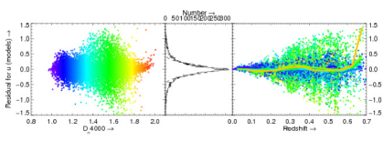
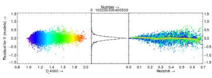
Tables with the coefficients for the approximation are in the Appendix (Tables A.1-A.4). Figure 9 shows the residuals as a function of and redshift for and . The thick colored lines indicate the median of the residuals binned by to show the absence of structure in the residuals as a function of redshift. Table 2 contains statistics ( of the Gaussian fit, rms, and the 68.3 % range around the mean) on the residuals for the fit.
We also determine the coefficients for our fit as a function of (now in eqs. [A2] and [A3]) and redshift in order to compare our results with CMZ10 (see Section 5). We show the residuals in Figure 10 for and . The coefficients for the approximation are in the Appendix (Tables A.5-A.8). Table 2 contains statistics on the residuals. We note that the analytic approximations using on show the same, or lower, residuals for the and bands, respectively, compared with those approximations of the same polynomial order based on .
5 Comparison with previous work
The advantage of using k-corrections determined directly from spectra relative to those from models or model fits is that we make no assumptions about galaxy evolution, attenuation laws, metallicities, orientation, etc. Using the spectra directly also eliminates the need for constructing a set of models that—in linear combination—represent fundamental galaxy types. However, models do not have the (photon)noise that the observations contain. Here, we compare our empirical k-corrections with the models of CMZ10.
Figure 8 shows the model tracks of pure SSP models from Figure 5 plotted over our data. The range of spectroscopically determined k-corrections matches the range of the models at the high end extremely well. At the low end, there are few galaxies with k-corrections as low as predicted by the youngest SSP models without attenuation. This difference implies that these low galaxies are always (significantly) attenuated and/or these galaxies rarely have a stellar population that consists purely of young stars.
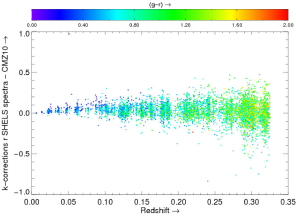
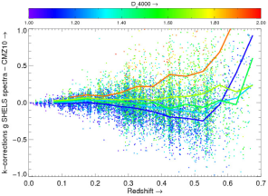
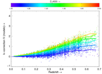
We next compare our k-corrections with those from the literature. CMZ10 provides k-corrections as a function of redshift and just one other parameter, the observed galaxy color. They use photometry in up to nine optical and near-infrared bands for galaxies with known redshift to fit a grid of SSP models from pegase.2 (Fioc & Rocca-Volmerange, 1997). In Figure 11 we show the k-corrections for our galaxies determined with the prescription of CMZ10.666Blanton & Roweis (2007) also provide a method to determine the k-corrections. The method of CMZ10 is similar to that of Blanton & Roweis (2007) in the sense that both use template spectra to fit the photometric data, but the template set of CMZ10 differs from the set of Blanton & Roweis (2007). Furthermore, CMZ10 do a detailed comparison and conclude that the results from both approaches are similar.
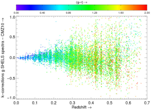
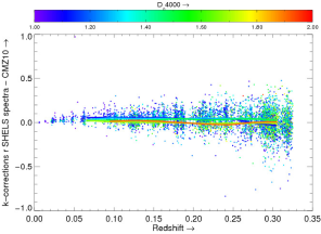
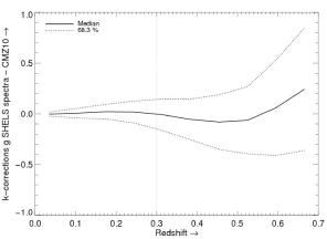
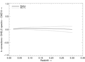
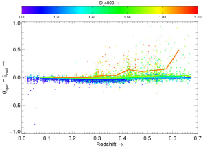
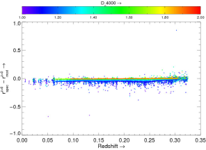
Figure 12 shows the difference between the k-corrections derived from our data and those from CMZ10 for SHELS galaxies as a function of both and . The k-corrections for the band agree extremely well. The k-corrections for the band also agree well up to (68.3 % range around the median difference is 0.15 and 0.12 for and , respectively at ). For larger , they start to disagree for galaxies with large . The cause for this difference is twofold.
At a redshift of 0.3, the CMZ10 sample does not contain as many green-to-blue galaxies as red galaxies. They drew their sample of galaxies from SDSS DR7 (Abazajian et al., 2009) and UKIRT Infrared Deep Sky Survey DR5 (Lawrence et al., 2007) with redshifts between 0.03 and 0.6. The galaxies in SDSS DR7 have spectroscopy for at least two distinct samples: the main galaxy sample () with a median redshift around 0.10 and the luminous red galaxy sample () selected with the majority of the galaxies at redshifts higher than 0.15.
In contrast, SHELS reaches much fainter than SDSS () and selects galaxies based only on their total magnitude. Thus, SHELS is not biased toward or against a particular type of galaxy (except against AGN due to their stellarlike morphology). SHELS contains more (in number) intrinsically bluer galaxies at higher redshifts than CMZ10.
CMZ10 only selects galaxies with redshifts up to 0.6. Thus, their fit is only valid to approximately that redshift; SHELS contains galaxies to .
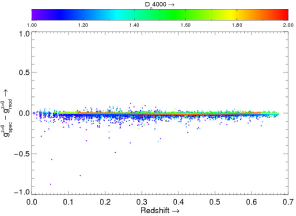
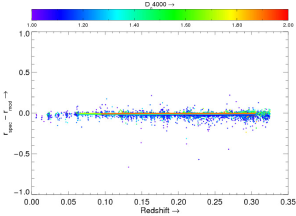
However, the differences with CMZ10 for the galaxies with the largest require further discussion. Figure 13 shows the differences between the magnitudes derived from the spectra and the models in the observed and rest frames. Modulo the presence of emission lines (Section 7) and noise, these magnitudes should be the same. Apart from the panel with observed -band magnitudes, all other panels show that the magnitudes derived from the spectra and the models are consistent with each other.
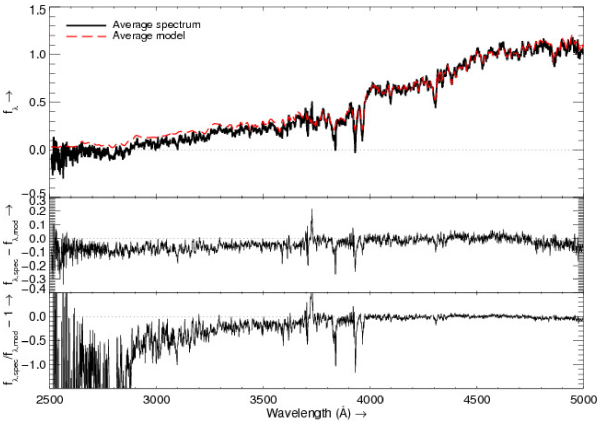
We investigate the overestimation in flux indicated by Figure 13 of the high- galaxies from the models with respect to the spectra by combining the spectra of these galaxies. We note that for the galaxies with the oldest stellar populations there is less flexibility in fitting the models than for galaxies with younger populations because only old SSP models can fit; for younger populations conceivably different combinations of young and old SSP models (and an increased/decreased amount of attenuation) can yield a good fit.
Figure 14 shows the averaged luminosity-weighted rest-frame spectrum—of both the actual spectra and the model fits—of 84 galaxies with , , and a difference between the magnitude derived from the spectrum and the fit that is larger than 0.2. We also show the difference between the averaged spectrum and averaged model in the middle panel and the relative difference between the averaged spectrum and averaged model with respect to the averaged model.
The models deviate from the spectra at the bluest rest-frame wavelengths. The relative difference there is large. Because the features in the average fit also appear in the spectrum, the flux of the average spectrum goes only marginally below 0. These rest-frame wavelengths correspond to the bluest part of the spectrum (where the spectrograph is not very sensitive) and it appears that the sky is somewhat oversubtracted. We suggest the use of the k-corrections determined from the model fits for the galaxies with high at the highest redshifts.
Overall, we find very good agreement between our k-corrections using the full spectrum and the prescription of CMZ10 based on SSP fits to photometry. Similar to CMZ10 (who use redshift and observed color), we can approximate the k-correction with only two parameters: redshift and . There are no systematics remaining in the residuals of our approximation.
6 Uncertainties
In Section 3.3 we determined from the model fits to the spectra. Not every spectrum is suitable for fitting SSP models; in those cases one can determine from the spectrum. In this section we consider the effects of using the spectrum-derived on the determination of the k-correction instead of using the model-derived . We compare the accuracy of the model-derived with the spectrum-derived .
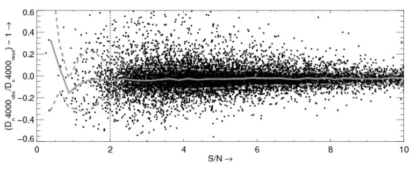
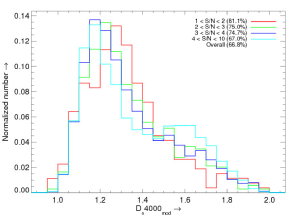
The accuracy of is obviously a function of the S/N of the spectrum. The S/N for each of our spectra is the median of the S/N per Hectospec pixel measured in 10 wavelength ranges in the observed spectrum that are free of night-sky emission and sample the range over which we fit our models to the spectrum (4100–4300, 5000–5200, 5470–5570, 5700–5850, 6000–6200, 6400–6600, 6650–6700, 7000–7200, 7600–7700, and 8050–8250 Å). Figure 15 shows the relative difference of the spectrum- and model-derived as a function of S/N. The accuracy of increases, as one might expect, with increasing S/N.
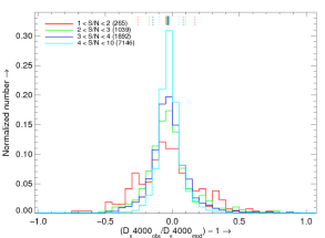
Figure 15 also shows the distribution of the relative difference between the model- and spectrum-derived binned by S/N. The 68.3 % range around the median increases with decreasing S/N (0.21, 0.13, 0.11, and 0.07, respectively, for the four S/N ranges indicated). The values of the higher S/N spectra are consistent with the comparison between SDSS and Hectospec spectra of Fabricant et al. (2008, ).
Figure 15 also shows the distribution of model-derived (because we use this throughout this article) in the same S/N bins. Galaxies with the most poorly determined are typically the low surface brightness—also intrinsically bluer—galaxies.
Table 3 shows the k-corrections and their uncertainties for a few example galaxies given the uncertainties in and . The three uncertainties for correspond to the 68.3 % range around the median for very low, moderate, and high S/N spectra. The uncertainties in the corresponding color are those in the SDSS Petrosian and fiber colors. The column indicates the corresponding range in the calculated k-correction. We choose the redshifts of the galaxies, and , close to the maximum redshifts where we can determine k-corrections for the and bands, respectively. We choose values that are typical for the two populations of galaxies (Fig. 6; and ).
The from a spectrum with () yields an uncertainty in the k-correction, similar to the uncertainty in the k-correction determined from given the typical uncertainties in the galaxy color. For the from a spectrum with (), the uncertainty in the k-correction is somewhat larger than the uncertainty in the k-correction determined from . In most of the examples, the uncertainty in the SDSS magnitude dominates the uncertainty in the final absolute magnitude, not the uncertainty in the k-correction.
7 Emission lines
Emission lines with large REW can significantly affect the flux density measured through a filter.777Narrowband surveys employ exactly this feature to increase the contrast between observations done with a very narrow filter and a broadband filter; the narrower the filter becomes, the larger the difference in magnitude between the two filters (e.g., Waller, 1990; Pascual et al., 2007). Figure 13 shows the influence of the emission lines on the magnitudes. The galaxies with low and are almost all emission-line galaxies.
As Woods et al. (2010) show (see also Section 3.3 and Figure 6), nearly all galaxies with low have emission lines. These galaxies make up a large fraction of our sample. We thus investigate the influence of the emission lines on the derived k-corrections.
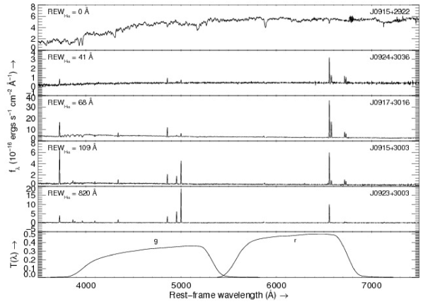
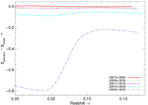
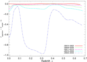
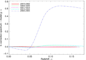
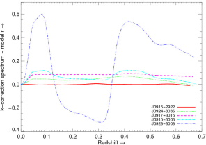
We examine five galaxies with differing emission-line REWs. Figure 16 shows the spectra of these galaxies. We calculate the magnitudes and k-corrections as a function of redshift from the rest-frame spectra and the model fits of these galaxies. We assume that the difference between the spectrum and the model results only from the emission lines. We plot the difference in derived magnitudes and k-corrections for both bands in Figure 17.888The spectra of these galaxies normally evolve over time. The point of this figure, however, is to demonstrate the influence of emission lines, not galaxy evolution.
The entrance and departure of emission lines from the filter as a function of increasing redshift dominate the curve that traces the difference in magnitudes. At the H and [O iii] 4959,5007 complex are in the filter and leave it with increasing redshift. Around the [Oii] 3726,3728 doublet enters the filter, causing the difference in the magnitude to increase only slightly. For the band, the rippling shape of the curve results from [S ii] 6733,6718, [N ii] 6550,6585, and (predominantly) H leaving the filter with increasing redshift and having left around , while the H and [O iii] complex starts to enter the filter at the same time. Around the complex starts to leave, while H enters. At H leaves and H enters.
Figure 17 shows that (1) the influence of emission lines is clearly correlated with their equivalent width, and (2) apart from galaxies with extremely large REW emission lines (Å), the influence of emission lines on the broadband and magnitudes—and, consequently, k-corrections—is reasonably small. The significance depends on the accuracy of the photometry and/or the required precision of the k-corrections. For an accuracy mag k-corrections need to take emission-line flux into account. For example, Brown et al. (2008) use the influence of strong emission lines on the observed galaxy colors to select extremely metal poor galaxies.
8 Additional k-corrections
In Section 4 we determined the k-corrections for the SDSS and bands; here we consider k-corrections in other photometric bands. Because emission lines are important for only the strongest emission lines in a galaxy spectrum and our model fit extends beyond the wavelength range of the spectrum, we can calculate the k-corrections for any optical bandpass over the redshift range where we sample enough galaxies: i.e., .
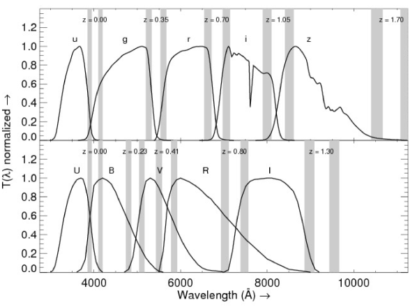
Here, we derive the k-corrections as a function of redshift and for the SDSS bandpasses and the Johnson-Cousins given in Table 2 of Bessell (1990). Figure 18 shows the 10 normalized bandpasses we used to calculate the k-corrections. Figure 19 showcases the results for the SDSS and the Johnson-Cousins band. The figures for these and the remaining filters are also available online.999See http://tdc-www.cfa.harvard.edu/instruments/hectospec/progs/EOK/figures.shtml. Tables A.9-A.18 contain the coefficients for the analytic approximation using redshift and , Tables A.19-A.23 contain the coefficients for the approximations using redshift and color (SDSS filters only; we do not have imaging available in the Johnson-Cousins bandpasses). We give the statistics of the residuals in Table 4 to indicate the quality of the fits.
For the bandpasses, our k-corrections match those of CMZ10 at for galaxies with high and at for galaxies with low . CMZ10 selects galaxies with redshifts up to 0.6 and their number of green galaxies decreases steeply beyond redshift 0.3. Furthermore, toward redder filters the differences between our k-corrections and those of CMZ10 decrease; because the 4000 Å break goes through the redder filters at higher redshifts, the k-corrections for the redder filters are also smaller than for the bluest filters.
The residuals from the analytic approximation using and redshift are about the same as or smaller than those using observed galaxy color and redshift. This result is, however, not surprising; the optical observed galaxy colors used by CMZ10 coarsely probe for the particular filter where they calculate the k-correction.
9 Summary
We use the 15,513 SHELS spectra to determine the k-corrections for the SDSS and bands empirically. These k-corrections have the major advantage that they are model-independent. We express the analytic approximations for the k-correction as a function of two parameters: redshift and . These parameters have some advantages over those from CMZ10: redshift and galaxy color. The advantages include (1) is redshift-independent, (2) is an indicator of the age of the stellar population of the galaxy, (3) barely suffers from attenuation, (4) the spectrum used to determine the redshift of a galaxy can also yield , and (5) the spectrum does not necessarily have to be flux-calibrated to determine . Furthermore, the analytic approximations based on have about the same ( band) or less scatter ( band), compared with the approximations using . The of the scatter in the residuals is mag, the rms is ; the residuals also show no systematic bias.
From CB07 SSP models we indicate the range of k-corrections that we determine from observed galaxies. The models with the youngest and oldest stellar populations with a small amount of attenuation span the entire range of determined k-corrections. We conclude that galaxies are always (significantly) attenuated and/or rarely have a stellar population that consists purely of young stars.
We compare our results to the analytic approximations given by CMZ10. Up to our results agree well for both bands. Differences between the two surveys arise due to the fact that SHELS goes to significantly fainter magnitudes than SDSS (the survey from which CMZ10 draws). Furthermore, our total magnitude selection criterion allows us to sample the entire range of galaxies up to , rather than selecting for luminous red galaxies (like SDSS). We make the analytic approximations available in an online calculator (see footnote 7).
We check the influence of emission lines on the k-corrections. The influence of the emission lines depends on the REW of the line; the larger the REW of the line, the larger the influence on the k-correction is. Depending on the accuracy of the k-corrections required, the influence of emission lines can typically be ignored, except those few cases in which the REW is very large ( Å gives mag).
Finally, we provide k-corrections as a function of redshift and using our model fits for SDSS and Johnson-Cousins . We determine these k-corrections over the redshift range where we sample enough galaxies: i.e., . We compare our results to the analytical approximations given by CMZ10 and show that we cover a larger redshift range, where we sample more (in number) “green” galaxies than CMZ10 do. For spectra with S/N 2 (), the k-corrections based on are as good as those based on color.
Despite the fact that the scatter in our k-corrections is typically mag, the uncertainties in the observed magnitude are of a similar size or larger. Thus, uncertainties in the magnitudes dominate the uncertainty in the final, k-corrected magnitude.
This empirical approach to determine k-corrections can be extended to the near- and midinfrared to include spectroscopic features, such as the Paschen and Brackett hydrogen lines (and breaks) and polycyclic aromatic hydrocarbon features. The technique can also be extended to higher redshifts where the 4000 Å break moves through the reddest optical filters and into the near-infrared.
Acknowledgments
EW acknowledges the Smithsonian Institution for the support of his postdoctoral fellowship.
Observations reported here were obtained at the MMT Observatory, a joint facility of the Smithsonian Institution and the University of Arizona. The SDSS is managed by the Astrophysical Research Consortium for the Participating Institutions.
We thank Susan Tokarz and Bill Wyatt for reducing and redshifting the Hectospec data, John Roll for actively maintaining and updating Starbase, Bill Wyatt for maintaining a local copy of the SDSS database. We acknowledge the work of the Hectospec instrument assistants Perry Berlind and Mike Calkins, and the MMT telescope operators Mike Alegria, John McAfee, and Ale Milone. We thank all the staff at the Telescope Data Center and Fred Lawrence Whipple Observatory that make the observations possible. We have benefited from discussions with Warren Brown, Nelson Caldwell, and Scott Kenyon.
Appendix A K-correction approximations: surface fitting
In Section 4 we describe the empirical k-correction as a result of redshift and either or color. Here, we describe the method used for the fitting and give the coefficients for the approximations.
We use minimization to determine the coefficients for our analytic approximations. We describe our method in the context of fitting a two-dimensional surface. The surface as a function of coordinates and is given by
| (A1) |
where are the coefficients and and are the maximum polynomial terms for and , respectively.
The for this surface for data points is defined as
| (A2) |
The minimization for each coefficient yields
| (A3) |
We solve these equations using lower/upper (LU) decomposition. For LU decomposition we need to write all equations from eq. [A3] as a linear system , where is a vector containing the coefficients. Let and , then the linear system we solve looks like
| (A4) |
We use the IDL routine la_linear_equation based on LAPACK (Anderson et al., 1999) to solve for .
We apply this method to the data presented in this article. The variables , , and represent the redshift, (or , depending on which of the two we fit), and the k-correction, respectively, for each individual galaxy. is the number of galaxies. We show the residuals of our fits in Figures 9, 10, and 19 and online (see footnote 11).
Tables A.1–A.23 contain the coefficients for the fits described in this article (similar to CMZ10, ). One calculates the k-correction by taking the index of the row multiplied with the index of the column (i.e., , or ), and multiplying that with the coefficient () in the table; one needs to do this for all coefficients in the table. The sum of those values is the k-correction for the given redshift and (or where appropriate). Note that no table contains a row with because we demand, by definition, that at redshift the k-correction is 0 (Section 1).
References
- Abazajian et al. (2009) Abazajian, K. N., Adelman-McCarthy, J. K., Agüeros, M. A., Allam, S. S., Allende Prieto, C., An, D., Anderson, K. S. J., Anderson, S. F., Annis, J., Bahcall, N. A., Bailer-Jones, C. A. L., Barentine, J. C., Bassett, B. A., Becker, A. C., & et al. (SDSS collaboration). 2009, ApJS, 182, 543
- Anderson et al. (1999) Anderson, E., Bai, Z., Bischof, C., Blackford, S., Demmel, J., Dongarra, J., Du Croz, J., Greenbaum, A., Hammarling, S., McKenney, A., & Sorensen, D. 1999, LAPACK Users’ Guide, 3rd edn. (Philadelphia, PA: Society for Industrial and Applied Mathematics)
- Balogh et al. (1999) Balogh, M. L., Morris, S. L., Yee, H. K. C., Carlberg, R. G., & Ellingson, E. 1999, ApJ, 527, 54
- Bessell (1990) Bessell, M. S. 1990, PASP, 102, 1181
- Blanton et al. (2001) Blanton, M. R., Dalcanton, J., Eisenstein, D., Loveday, J., Strauss, M. A., SubbaRao, M., Weinberg, D. H., Anderson, Jr., J. E., Annis, J., Bahcall, N. A., Bernardi, M., Brinkmann, J., Brunner, R. J., Burles, S., Carey, L., Castander, F. J., Connolly, A. J., Csabai, I., Doi, M., Finkbeiner, D., Friedman, S., Frieman, J. A., Fukugita, M., Gunn, J. E., Hennessy, G. S., Hindsley, R. B., Hogg, D. W., Ichikawa, T., Ivezić, Ž., Kent, S., Knapp, G. R., Lamb, D. Q., Leger, R. F., Long, D. C., Lupton, R. H., McKay, T. A., Meiksin, A., Merelli, A., Munn, J. A., Narayanan, V., Newcomb, M., Nichol, R. C., Okamura, S., Owen, R., Pier, J. R., Pope, A., Postman, M., Quinn, T., Rockosi, C. M., Schlegel, D. J., Schneider, D. P., Shimasaku, K., Siegmund, W. A., Smee, S., Snir, Y., Stoughton, C., Stubbs, C., Szalay, A. S., Szokoly, G. P., Thakar, A. R., Tremonti, C., Tucker, D. L., Uomoto, A., Vanden Berk, D., Vogeley, M. S., Waddell, P., Yanny, B., Yasuda, N., & York, D. G. 2001, AJ, 121, 2358
- Blanton & Roweis (2007) Blanton, M. R. & Roweis, S. 2007, AJ, 133, 734
- Brown et al. (2008) Brown, W. R., Kewley, L. J., & Geller, M. J. 2008, AJ, 135, 92
- Bruzual (2006) Bruzual, A. G. 2006, Proceedings of the International Astronomical Union, 2, 125
- Bruzual (1983) Bruzual, G. 1983, ApJ, 273, 105
- Bruzual & Charlot (2003) Bruzual, G. & Charlot, S. 2003, MNRAS, 344, 1000
- Calzetti et al. (2000) Calzetti, D., Armus, L., Bohlin, R. C., Kinney, A. L., Koornneef, J., & Storchi-Bergmann, T. 2000, ApJ, 533, 682
- Charlot & Fall (2000) Charlot, S. & Fall, S. M. 2000, ApJ, 539, 718
- Chilingarian et al. (2010) Chilingarian, I., Melchior, A., & Zolotukhin, I. 2010, ArXiv e-prints
- Fabricant et al. (2005) Fabricant, D., Fata, R., Roll, J., Hertz, E., Caldwell, N., Gauron, T., Geary, J., McLeod, B., Szentgyorgyi, A., Zajac, J., Kurtz, M., Barberis, J., Bergner, H., Brown, W., Conroy, M., Eng, R., Geller, M., Goddard, R., Honsa, M., Mueller, M., Mink, D., Ordway, M., Tokarz, S., Woods, D., Wyatt, W., Epps, H., & Dell’Antonio, I. 2005, PASP, 117, 1411
- Fabricant et al. (1998) Fabricant, D. G., Hertz, E. N., Szentgyorgyi, A. H., Fata, R. G., Roll, J. B., & Zajac, J. M. 1998, in Presented at the Society of Photo-Optical Instrumentation Engineers (SPIE) Conference, Vol. 3355, Society of Photo-Optical Instrumentation Engineers (SPIE) Conference Series, ed. S. D’Odorico, 285–296
- Fabricant et al. (2008) Fabricant, D. G., Kurtz, M. J., Geller, M. J., Caldwell, N., Woods, D., & Dell’Antonio, I. 2008, PASP, 120, 1222
- Fioc & Rocca-Volmerange (1997) Fioc, M. & Rocca-Volmerange, B. 1997, A&A, 326, 950
- Geller et al. (2005) Geller, M. J., Dell’Antonio, I. P., Kurtz, M. J., Ramella, M., Fabricant, D. G., Caldwell, N., Tyson, J. A., & Wittman, D. 2005, ApJ, 635, L125
- Geller et al. (2010) Geller, M. J., Kurtz, M. J., Dell’Antonio, I. P., Ramella, M., & Fabricant, D. G. 2010, ApJ, 709, 832
- Hogg et al. (2002) Hogg, D. W., Baldry, I. K., Blanton, M. R., & Eisenstein, D. J. 2002, ArXiv Astrophysics e-prints
- Hubble (1936) Hubble, E. 1936, ApJ, 84, 517
- Kauffmann et al. (2003) Kauffmann, G., Heckman, T. M., White, S. D. M., Charlot, S., Tremonti, C., Brinchmann, J., Bruzual, G., Peng, E. W., Seibert, M., Bernardi, M., Blanton, M., Brinkmann, J., Castander, F., Csábai, I., Fukugita, M., Ivezic, Z., Munn, J. A., Nichol, R. C., Padmanabhan, N., Thakar, A. R., Weinberg, D. H., & York, D. 2003, MNRAS, 341, 33
- Kewley et al. (2005) Kewley, L. J., Jansen, R. A., & Geller, M. J. 2005, PASP, 117, 227
- Kurtz et al. (2007) Kurtz, M. J., Geller, M. J., Fabricant, D. G., Wyatt, W. F., & Dell’Antonio, I. P. 2007, AJ, 134, 1360
- Kurtz & Mink (1998) Kurtz, M. J. & Mink, D. J. 1998, PASP, 110, 934
- Lawrence et al. (2007) Lawrence, A., Warren, S. J., Almaini, O., Edge, A. C., Hambly, N. C., Jameson, R. F., Lucas, P., Casali, M., Adamson, A., Dye, S., Emerson, J. P., Foucaud, S., Hewett, P., Hirst, P., Hodgkin, S. T., Irwin, M. J., Lodieu, N., McMahon, R. G., Simpson, C., Smail, I., Mortlock, D., & Folger, M. 2007, MNRAS, 379, 1599
- Mink et al. (2007) Mink, D. J., Wyatt, W. F., Caldwell, N., Conroy, M. A., Furesz, G., & Tokarz, S. P. 2007, in Astronomical Society of the Pacific Conference Series, Vol. 376, Astronomical Data Analysis Software and Systems XVI, ed. R. A. Shaw, F. Hill, & D. J. Bell, 249–+
- Muller et al. (1998) Muller, G. P., Reed, R., Armandroff, T., Boroson, T. A., & Jacoby, G. H. 1998, in Presented at the Society of Photo-Optical Instrumentation Engineers (SPIE) Conference, Vol. 3355, Society of Photo-Optical Instrumentation Engineers (SPIE) Conference Series, ed. S. D’Odorico, 577–585
- Oke & Gunn (1983) Oke, J. B. & Gunn, J. E. 1983, ApJ, 266, 713
- Pascual et al. (2007) Pascual, S., Gallego, J., & Zamorano, J. 2007, PASP, 119, 30
- Roll et al. (1998) Roll, J. B., Fabricant, D. G., & McLeod, B. A. 1998, in Society of Photo-Optical Instrumentation Engineers (SPIE) Conference Series, Vol. 3355, Society of Photo-Optical Instrumentation Engineers (SPIE) Conference Series, ed. S. D’Odorico, 324–332
- Steidel et al. (1995) Steidel, C. C., Pettini, M., & Hamilton, D. 1995, AJ, 110, 2519
- Tremonti et al. (2004) Tremonti, C. A., Heckman, T. M., Kauffmann, G., Brinchmann, J., Charlot, S., White, S. D. M., Seibert, M., Peng, E. W., Schlegel, D. J., Uomoto, A., Fukugita, M., & Brinkmann, J. 2004, ApJ, 613, 898
- Waller (1990) Waller, W. H. 1990, PASP, 102, 1217
- Westra et al. (2010) Westra, E., Geller, M. J., Kurtz, M. J., Fabricant, D. G., & Dell’Antonio, I. 2010, ApJ, 708, 534
- Wittman et al. (2006) Wittman, D., Dell’Antonio, I. P., Hughes, J. P., Margoniner, V. E., Tyson, J. A., Cohen, J. G., & Norman, D. 2006, ApJ, 643, 128
- Wittman et al. (2002) Wittman, D. M., Tyson, J. A., Dell’Antonio, I. P., Becker, A., Margoniner, V., Cohen, J. G., Norman, D., Loomba, D., Squires, G., Wilson, G., Stubbs, C. W., Hennawi, J., Spergel, D. N., Boeshaar, P., Clocchiatti, A., Hamuy, M., Bernstein, G., Gonzalez, A., Guhathakurta, P., Hu, W., Seljak, U., & Zaritsky, D. 2002, in Society of Photo-Optical Instrumentation Engineers (SPIE) Conference Series, Vol. 4836, Society of Photo-Optical Instrumentation Engineers (SPIE) Conference Series, ed. J. A. Tyson & S. Wolff, 73–82
- Woods et al. (2010) Woods, D. F., Geller, M. J., Kurtz, M. J., Westra, E., Fabricant, D. G., & Dell’Antonio, I. 2010, AJ, 139, 1857
- Yasuda et al. (2001) Yasuda, N., Fukugita, M., Narayanan, V. K., Lupton, R. H., Strateva, I., Strauss, M. A., Ivezić, Ž., Kim, R. S. J., Hogg, D. W., Weinberg, D. H., Shimasaku, K., Loveday, J., Annis, J., Bahcall, N. A., Blanton, M., Brinkmann, J., Brunner, R. J., Connolly, A. J., Csabai, I., Doi, M., Hamabe, M., Ichikawa, S., Ichikawa, T., Johnston, D. E., Knapp, G. R., Kunszt, P. Z., Lamb, D. Q., McKay, T. A., Munn, J. A., Nichol, R. C., Okamura, S., Schneider, D. P., Szokoly, G. P., Vogeley, M. S., Watanabe, M., & York, D. G. 2001, AJ, 122, 1104
Facilities: MMT (Hectospec)
| Age | ||
|---|---|---|
| 5 Myr | 0.0 | 0.94 |
| 25 Myr | 0.0 | 0.97 |
| 100 Myr | 0.0 | 1.05 |
| 250 Myr | 0.0 | 1.13 |
| 500 Myr | 0.0 | 1.26 |
| 1.0 Gyr | 0.0 | 1.41 |
| 1.4 Gyr | 0.0 | 1.45 |
| 2.5 Gyr | 0.0 | 1.58 |
| 5.0 Gyr | 0.0 | 1.77 |
| 10.0 Gyr | 0.0 | 1.96 |
| 5 Myr | 1.0 | 0.98 |
| 10.0 Gyr | 0.5 | 2.00 |
Note. — These models are indicated in Fig. 5.
| filter | rms | 68.3 % | rms | 68.3 % | ||
|---|---|---|---|---|---|---|
| Spectra | ||||||
| 0.08 | 0.17 | 0.11 | 0.12 | 0.25 | 0.17 | |
| 0.08 | 0.12 | 0.09 | 0.07 | 0.11 | 0.08 | |
| Models | ||||||
| 0.09 | 0.14 | 0.11 | 0.12 | 0.21 | 0.16 | |
| 0.07 | 0.10 | 0.08 | 0.06 | 0.09 | 0.07 | |
Note. — is the of the Gaussian fit to the residuals for the analytic approximations to the k-corrections derived from the spectra and the models for and with and 0.33, respectively, as a function of and ; rms is the rms of the residuals; 68.3 % is the range around the mean of the residuals. Figures 9 and 10 show the residuals and the Gaussian fits to the residuals.
| filter | |||||||||||||||||
|---|---|---|---|---|---|---|---|---|---|---|---|---|---|---|---|---|---|
| 0.30 | 1.25 | 0.15 | 0.09 | 0.61 | 0.21 | 0.11 | 0.07 | 0.97 | 0.61 | 0.17 | 0.10 | ||||||
| 0.30 | 1.65 | 0.18 | 0.11 | 1.15 | 0.21 | 0.11 | 0.07 | 1.48 | 1.12 | 0.20 | 0.11 | ||||||
| 0.30 | 1.25 | 0.09 | 0.06 | 0.21 | 0.21 | 0.11 | 0.07 | 0.97 | 0.21 | 0.17 | 0.10 | ||||||
| 0.30 | 1.65 | 0.08 | 0.04 | 0.41 | 0.21 | 0.11 | 0.07 | 1.48 | 0.42 | 0.20 | 0.11 | ||||||
| 0.55 | 1.25 | 0.29 | 0.15 | 1.08 | 0.21 | 0.11 | 0.07 | 1.04 | 1.29 | 0.32 | 0.17 | ||||||
| 0.55 | 1.65 | 0.47 | 0.24 | 2.24 | 0.21 | 0.11 | 0.07 | 1.65 | 2.06 | 0.49 | 0.25 |
Note. — and are the typical for the SDSS Petrosian and fiber magnitude of a galaxy with chosen and redshift . The uncertainties are those typical for very low, moderate and high S/N spectra. is the range in the calculated k-correction corresponding to the uncertainty in (or ). is the typical galaxy color for the chosen and redshift, and and are the typical uncertainties in the SDSS Petrosian and fiber color, respectively, for such a galaxy.
| Color | |||||||
|---|---|---|---|---|---|---|---|
| filter | rms | 68.3 % | color | rms | 68.3 % | ||
| 0.16 | 0.30 | 0.22 | 0.30 | 0.48 | 0.55 | ||
| 0.09 | 0.11 | 0.14 | 0.12 | 0.22 | 0.16 | ||
| 0.10 | 0.15 | 0.12 | 0.09 | 0.17 | 0.12 | ||
| 0.10 | 0.15 | 0.12 | 0.09 | 0.14 | 0.11 | ||
| 0.09 | 0.14 | 0.11 | 0.09 | 0.14 | 0.11 | ||
| 0.16 | 0.30 | 0.22 | … | … | … | … | |
| 0.10 | 0.17 | 0.13 | … | … | … | … | |
| 0.10 | 0.14 | 0.12 | … | … | … | … | |
| 0.10 | 0.15 | 0.12 | … | … | … | … | |
| 0.09 | 0.15 | 0.12 | … | … | … | … | |
Note. — The table headings are the same as Table 2. The figures at http://tdc-www.cfa.harvard.edu/instruments/hectospec/progs/EOK/figures.shtml show the residuals and the Gaussian fits to the residuals. Figure 19 shows the figures for and .
| 29.9754 | -78.4292 | 64.0436 | -15.8884 | |
| -368.572 | 818.057 | -581.89 | 134.427 | |
| 490.834 | -1084.35 | 768.318 | -176.591 |
| 6.6812 | -27.6858 | 27.7299 | -7.319 | |
| -231.313 | 517.183 | -364.586 | 82.7252 | |
| 330.803 | -735.254 | 517.408 | -117.366 |
| 25.4725 | -52.2513 | 35.6903 | -7.85585 | |
| -177.822 | 336.276 | -203.045 | 39.6419 | |
| 66.6927 | -82.7486 | 7.78744 | 9.65736 |
| -2.4549 | 3.08855 | -0.85258 | 0.169083 | |
| 31.7806 | -96.6607 | 92.3012 | -26.9024 | |
| -334.912 | 776.204 | -593.901 | 148.071 |
| 0.126452 | 0.0619892 | 6.90796 | -2.98031 | |
| 3.51286 | -9.40049 | -9.17117 | 6.52303 | |
| -8.56012 | 24.3121 | -2.88499 | -3.57257 |
| -0.160448 | 1.12881 | 5.93095 | -2.68308 | |
| 4.04345 | -11.8962 | -6.0987 | 5.37315 | |
| -9.01521 | 26.6088 | -6.50937 | -2.17746 |
| 2.30349 | -7.69531 | 11.1784 | -4.33398 | |
| -20.1966 | 77.9084 | -88.5243 | 31.1532 | |
| 21.5438 | -130.494 | 156.555 | -54.8953 |
| -0.823562 | 1.8179 | 1.8466 | -1.21972 | |
| 6.54473 | -13.4719 | 3.54192 | 1.11608 | |
| -28.7761 | 59.0299 | -39.6835 | 8.96288 |
| 2.43154 | -16.3322 | 20.0889 | -6.24137 | |
| -52.0421 | 120.631 | -101.738 | 31.5506 | |
| 147.367 | -326.482 | 247.473 | -66.0534 |
| 7.12187 | -28.8064 | 28.6961 | -7.57514 | |
| -234.056 | 523.817 | -370.133 | 84.1717 | |
| 333.917 | -742.667 | 523.643 | -118.999 |
| 3.90822 | -11.2489 | 10.1242 | -2.60069 | |
| -134.442 | 274.564 | -182.224 | 39.2976 | |
| 165.269 | -339.815 | 227.173 | -48.4853 |
| 24.114 | -53.0651 | 38.4687 | -8.97268 | |
| -231.287 | 488.825 | -334.771 | 74.5591 | |
| 292.203 | -618.56 | 423.008 | -93.5608 |
| 14.5525 | -32.5735 | 24.1581 | -5.70902 | |
| -203.691 | 433.748 | -298.226 | 66.4327 | |
| 272.826 | -580.065 | 397.471 | -87.9759 |
| -9.40727 | 10.8489 | 0.644962 | -1.85733 | |
| -16.6686 | 36.2742 | -38.3145 | 16.2542 | |
| 113.958 | -246.016 | 185.69 | -50.5656 |
| -30.9335 | 56.0725 | -30.7097 | 5.99606 | |
| -61.7054 | 140.634 | -100.957 | 22.3406 | |
| 165.231 | -369.545 | 261.328 | -58.2109 |
| 12.8942 | -33.7534 | 26.7974 | -6.63462 | |
| -190.187 | 396.174 | -262.704 | 57.944 | |
| 217.218 | -449.526 | 298.181 | -65.3664 |
| 12.4246 | -29.1592 | 22.4394 | -5.40824 | |
| -175.969 | 366.836 | -248.343 | 54.7488 | |
| 218.881 | -457.84 | 310.701 | -68.0011 |
| 15.6639 | -34.3478 | 25.0727 | -5.82947 | |
| -196.21 | 412.661 | -280.861 | 61.9077 | |
| 256.842 | -540.797 | 367.306 | -80.3907 |
| 2.80197 | -5.1719 | 3.01032 | -0.447618 | |
| -16.0821 | 25.7573 | -10.8789 | 1.60111 | |
| 17.9556 | -26.6165 | 11.3526 | -1.79009 |
| 0.184129 | 1.00938 | 5.40158 | -2.41043 | |
| 0.112299 | -6.17196 | -7.21778 | 4.89703 | |
| -2.37339 | 15.3331 | -1.95179 | -2.36049 |
| -0.196478 | 3.11481 | 0.486552 | -1.12639 | |
| -5.4512 | -6.547 | 1.09495 | 2.90943 | |
| 7.81183 | 8.41136 | -3.05571 | -2.2226 |
| 0.0678646 | 2.034 | -1.09155 | 0.110666 | |
| -7.44388 | 4.05582 | 0.521655 | -0.136389 | |
| 10.1914 | -9.5645 | 2.07254 | -0.160024 |
| 0.269465 | -0.496672 | 1.43921 | -0.220175 | |
| 0.935489 | 3.91534 | -5.03895 | 0.274978 | |
| -2.15467 | -3.71225 | 5.19059 | -0.292333 |
