Induced parameter-dependent optimization method applied to reaction rate determination

Abstract

Parameter fitting of data to a proposed equation almost always consider these parameters as independent variables. Here, the method proposed optimizes an arbitrary number of variables by the minimization of a function of a single variable. Such a technique avoids problems associated with multiple minima and maxima because of the large number of parameters, and could increase the accuracy of the determination by cutting down on machine errors. An algorithm for this optimization scheme is provided and applied to the determination of the rate constant and final concentration parameters for a first order and second order chemical reaction.

1 Introduction

Deterministic laws of nature are sometimes written - for the simplest examples- in the form

$$Y_{law}=Y_{law}(\mathbf{P},k,t)$$ (1)

linking the variable $Y_{law}$ to $t$. The components of $\mathbf{P}$, $P_{i}(i=1,2,...N_{p})$ and $k$ are parameters. Verification of a law of form (1) relies on an experimental dataset $\{(Y_{exp}(t_{i}),\,t_{i}),i=1,2,...N)\}$. Confirmation or verification of the law is based on (a) deriving suitable values for the parameters $(\mathbf{P},k)$ and (b) showing a good enough degree of fit between the experimental set $Y_{exp}(t_{i})$ and $Y_{law}(t_{i})$. Many methods [1, 2, 3, 4, etc.] have been devised to determine the optimal $\mathbf{P},k$ parameters, but most if not all these methods consider the aforementioned parameters as autonomous and independent (e.g. [2]) subjected to free and independent variation during the optimization process. On the other hand, if one considers the interplay between the experimental data and $Y_{law}$ one can derive certain parameters like the final concentration terms (e.g. $\lambda_{\infty}$ and $Y_{\infty}$ in what follows in sec.(3) ) if $k$, the rate constant is known. To preserve the viewpoint of the inter-relationship between these parameters and the experimental data, we devise a scheme that relates $\mathbf{P}$ to $k$ for all $P_{i}$ via the set $\{Y_{exp}(t_{i}),t_{i}\}$, and optimize the fit over $k$-space only. i.e. there is induced a $P_{i}(k)$ dependency on $k$ via the the experimental set $\{Y_{exp}(t_{i}),t_{i}\}$. it is unclear at present whether this optimization procedure is equivalent to previous ones, but its structure is not in contradiction with situations where there are inter-relations between the variables, and the results for the first and second order kinetics presented here are in very close agreement with those derived from the published literature. the advantages of the present method is that the optimization is over $1\,D$ $k$ space, leading to a unique determination of $\mathbf{P}$ with respect to $k$, whereas if all $\mathbf{P}$ are considered equally free, the optimization could lead to many different local solutions for each of the $\{P_{i}\}$. In what follows here, we assume that the rate laws and rate constants are not slowly varying functions of the reactant or product concentrations, which has recently from simulation been shown generally not to be the case [5].

2 Outline of Method

As above, $N$ is the number of dataset pairs $\{Y_{exp}(t_{i}),t_{i}\}$, $N_{p}$ the number of components of the $\mathbf{P}$ parameter, and $N_{s}$ the number of singularities where the use od a particular dataset $(Y_{exp},t)$leads to a singularity in the determination of $\bar{P}_{i}(k)$ as defined below and which must be excluded from being used in the determination of $\bar{P}_{i}(k)$. Then $(N_{p}+1)\leq(N-N_{s})$ for the unique determination of $\{\mathbf{P},k\}$. Define ${}^{N-N_{s}}C_{N_{p}}=N_{c}$ as the total number of combinations of the data-sets $\{Y_{exp}(t_{i}),t_{i}\}$ taken $N_{p}$ at a time that does not lead to singularities in $P_{i}$. Write $Y_{law}$ in the form

$$Y_{law}(t,k)=f(\mathbf{P},t,k).$$ (2)

Then map $f\longrightarrow Y_{th}(\bar{\mathbf{P}},t,k)$ as follows

$$Y_{th}(t,k)=f(\bar{\mathbf{P}},t,k)$$ (3)

where the term $\bar{\mathbf{P}}$ and its components is defined below and where $k$ is a varying parameter. For any of the $(i_{1},i_{2},\ldots,i_{N_{p}})$ combinations where $i_{j}\equiv(Yexp(t_{i_{j}}),t_{i_{j}})$ is a particular dataset pair, it is in principle possible to solve for the components of $\bar{\mathbf{P}}$ in terms of $k$ through the following simultaneous equations:

$$\begin{array}[]{rll}Y_{exp}(t_{i_{1}})&=&f(\mathbf{P},t_{i_{1}},k)\\[14.22636pt] Y_{exp}(t_{i_{2}})&=&f(\mathbf{P},t_{i_{2}},k)\\ &\vdots&\\ Y_{exp}(t_{i_{N_{p}}})&=&f(\mathbf{P},t_{i_{N_{p}}},k)\end{array}$$ (4)

For each $P_{i}$, there will be $N_{c}$ different solutions, $P_{i}(k,1),P_{i}(k,2),\ldots P_{i}(k,N_{c})$ . We can define (there are several possible mean definitions) an arithmetic mean for the components of $\bar{\mathbf{P}}$ as

$$\bar{P_{i}}(k)=\frac{1}{N_{c}}\sum_{i=1}^{N_{c}}P_{i}(k,j).$$ (5)

Each $P_{i}(k,j)$ is a function of $k$ whose derivative is known either analytically or by numerical differentiation. To derive an optimized set, then for the least squares method, define

$$Q(k)=\sum_{i=1^{\prime}}^{N^{\prime}}(Yexp(t_{i})-Y_{th}(k,t_{i}))^{2}.$$ (6)

Then for an optimized $k$, we have $Q^{\prime}(k)=0.$ Defining

$$P_{k}(k)=\sum_{i=1^{\prime}}^{N^{\prime}}(Y_{exp}(t_{i})-Y_{th}(k,t_{i})).Y_{th}^{\prime}(k,t_{i})$$ (7)

the optimized solution of $k$ corresponds to $P_{k}(k)=0.$ The most stable numerical solution is gotten by the bisection method where a solution is assured if the initial values of $k$ yield opposite signs for $P_{k}(k).$ Since all $\bar{P_{i}(k)}$ functions are known, their values may all be computed for one optimized $k$ value of $Q$ in (6). For a perfect fit of $Y_{exp}$ with $Y_{law}$, $Q(k^{\prime})=Q^{\prime}(k^{\prime})=0\Rightarrow\bar{P_{j}}\rightarrow\,P_{j}\,\,(\forall j)$ and so in this sense we define the above algorithm as giving optimized values for all $P_{i}$ parameters via the $k$ determination. This method is illustrated for the determination of two parameters in chemical reaction rate studies, of $1^{\mbox{st}}$ and $2^{\mbox{nd}}$ order respectively using data from published literature , where this method yields values very close to those quoted in the literature.

3 Applications in Chemical Kinetics

The first order reaction studied here is
(i) the methanolysis of ionized phenyl salicylate with data derived from the literature [6, Table 7.1,p.381]
and the second order reaction analyzed is
(ii) the reaction between plutonium(VI) and iron(II) according to the data in [7, Table II p.1427] and [8, Table 2-4, p.25].

3.1 First order results

Reaction (i) above corresponds to

$$\mbox{PS}^{-}+\mbox{CH${}_{3}$OH}\,\,\stackrel{{\scriptstyle k_{a}}}{{\longrightarrow}}\,\,\mbox{MS}^{-}+\mbox{PhOH}$$ (8)

where the rate law is pseudo first-order expressed as

$$\mbox{rate}=k_{a}\mbox{[PS]}^{-}=k_{c}[\mbox{CH${}_{3}$OH}][\mbox{PS}^{-}].$$

with the concentration of methanol held constant (80% v/v) and where the physical and thermodynamical conditions of the reaction appears in [6, Table 7.1,p.381]. The change in time $t$ for any material property $\lambda(t)$, which in this case is the Absorbance $A(t)$ (i.e. $A(t)\equiv\lambda(t)$is given by

$$\lambda(t)=\lambda_{\infty}-(\lambda_{\infty}-\lambda_{0})\exp{(-k_{a}t)}$$ (9)

for a first order reaction where $\lambda_{0}$ refers to the measurable property value at time $t=0$ and $\lambda_{\infty}$ is the value at $t=\infty$ which is usually treated as a parameter to yield the best least squares fit even if its optimized value is less for monotonically increasing functions (for positive $\frac{d\lambda}{dt}$at all $t$) than an experimentally determined $\lambda(t)$ at time $t$. In Table 7.1 of [6] for instance, $A(t=2160s)=0.897>A_{opt,\infty}=0.882$ and this value of $A_{\infty}$ is used to derive the best estimate of the rate constant as $16.5\pm 0.1\times 10^{-3}\mbox{sec}^{-1}$.
For this reaction, the $P_{i}$ of (2) refers to $\lambda_{\infty}$ so that $\mathbf{P}\equiv\lambda_{\infty}$ with $N_{p}=1$ and $k\equiv k_{a}$. To determine the parameter $\lambda_{\infty}$ as a function of $k_{a}$ according to (6) based on the entire experimental $\{(\lambda_{exp},t_{i})\}$ data set we invert (9) and write

$$\lambda_{\infty}(k)=\frac{1}{N^{\prime}}\sum_{i=1^{\prime}}^{N^{\prime}}\frac{(\lambda_{exp}(t_{i})-\lambda_{o}\exp{-kt_{i}})}{(1-\exp{-kt_{i}})}$$ (10)

where the summation is for all the values of the experimental dataset that does not lead to singularities, such as when $t_{i}=0$, so that here $N_{s}=1$. We define the non-optimized, continuously deformable theoretical curve $\lambda_{th}$ where $\lambda_{th}\equiv Y_{th}(t,k)$ in (3) as

$$\lambda_{th}(t,k)=\lambda_{\infty}(k)-(\lambda_{\infty}(k)-\lambda_{0})\exp{(-k_{a}t)}$$ (11)

With such a projection of the $\lambda_{\infty}$ parameter $P$ onto $k$, we seek the least square minimum of $Q_{1}(k)$, where $Q_{1}(k)\equiv Q$ of (6) for this first-order rate constant k in the form

$$Q_{1}(k)=\sum_{i=1}^{N}(\lambda_{exp}(t_{i})-\lambda_{th}(t_{i},k))^{2}$$ (12)

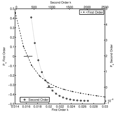
where the summation is over all the experimental $(\lambda_{exp}(t_{i}),t_{i})$ values. The resulting $P_{k}$ function (7) for the first order reaction based on the published dataset is given in Fig.(2).The solution of the rate constant $k$ corresponds to the zero value of the function, which exists for both orders. The $\mathbf{P}$ parameters ($\lambda_{\infty}$ and $Y_{\infty}$ ) are derived by back substitution into eqs. (10) and (15) respectively. The Newton-Raphson (NR) numerical procedure [9, p.362]was used to find the roots to $P_{k}$.For each dataset, there exists a value for $\lambda_{\infty}$ and so the error expressed as a standard deviation may be computed. The tolerance in accuracy for the NR procedure was $1.\times 10^{-10}$ . We define the function deviation $fd$ as the standard deviation of the experimental results with the best fit curve $fd=\surd\frac{1}{N}\{\sum_{i=1}^{N}(\lambda_{exp}(t_{i})-\lambda_{th}(t_{i})^{2}\}$ Our results are as follows:
$k_{a}=1.62\pm.09\times 10^{-2}\mbox{s}^{-1}$; $\lambda_{\infty}=0.88665\pm.006$; and $fd=3.697\times 10^{-3}$.
The experimental estimates are :
$k_{a}=1.65\pm.01\times 10^{-2}\mbox{s}^{-1}$; $\lambda_{\infty}=0.882\pm 0.0$; and $fd=8.563\times 10^{-3}$.
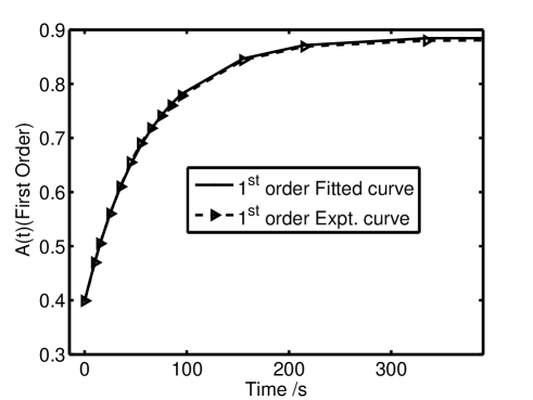
The experimental method involves adjusting the $A_{\infty}\equiv\lambda_{\infty}$ to minimize the $fd$ function and hence no estimate of the error in $A_{\infty}$ could be made. It is clear that our method has a lower $fd$ value and is thus a better fit, and the parameter values can be considered to coincide with the experimental estimates within experimental error. Fig.(1)shows the close fit between the curve due to our optimization procedure and experiment. The slight variation between the two curves may well be due to experimental uncertainties.

Figure 1: Plot of the experimental and curve with optimized parameters showing the very close fit between the two. The slight difference between the two can probably be attributed to experimental errors.

Figure 2: $P_{k}$ functions (7) for reactions (i) and (ii) of order one and two in reaction rate.

3.2 Second order results

To further test our method, we also analyze the second order reaction

$$\mbox{Pu(VI)}+2\mbox{Fe(II)}\,\,\stackrel{{\scriptstyle k_{b}}}{{\longrightarrow}}\,\,\mbox{Pu(IV)}+2\mbox{Fe(III)}$$ (13)

whose rate is given by $\mbox{rate}=k_{0}[\mbox{PuO}^{2+}_{2}][\mbox{Fe}^{2+}]$ where $k_{0}$ is relative to the constancy of other ions in solution such as $\mbox{H}^{+}$. The equations are very different in form to the first-order expressions and serves to confirm the viability of the current method.

For Espenson, the above stoichiometry is kinetically equivalent to the reaction scheme [8, eqn. (2-36)]

$$\mbox{PuO}_{2}^{2+}+\mbox{Fe}^{2+}_{aq}\stackrel{{\scriptstyle k_{b}}}{{\longrightarrow}}\,\mbox{PuO}^{+}_{2}+\mbox{Fe}^{3+}_{aq}.$$

which also follows from the work of Newton et al. [7, eqns. (8,9),p.1429] whose data [7, TABLE II,p.1427] we use and analyze to verify the principles presented here. Espenson had also used the same data as we have to derive the rate constant and other parameters [8, pp.25-26] which is used to check the accuracy of our methodology. The overall absorbance in this case $Y(t)$ is given by [8, eqn(2-35)]

$$Y(t)=\frac{Y_{\infty}+\left\{Y_{0}\left(1-\alpha\right)-Y_{\infty}\right\}\exp(-k\Delta_{0}t)}{1-\alpha\exp(-k\Delta_{0}t)}$$ (14)

where $\alpha=\frac{[\text{A}]_{0}}{[\text{B}]_{0}}$ is the ratio of initial concentrations where $[\text{B}]_{0}>[\text{A}]_{0}$ and $[\text{B}]=[\mbox{Pu(VI)}]$, $[\text{A}]=[\mbox{Fe(II)}]$ and $[\text{B}]_{0}=4.47\times 10^{-5}\text{M}$ and $[\text{A}]_{0}=3.82\times 10^{-5}\text{M}$ . A rearrangement of (14) leads to the equivalent expression [8, eqn(2-34)]

$$\ln\left\{1+\frac{\Delta_{0}\left(Y_{0}-Y_{\infty}\right)}{[\text{A}]_{0}\left(Y_{t}-Y_{\infty}\right)}\right\}=\ln\frac{[\text{B}]_{0}}{[\text{A}]_{0}}+k\Delta_{0}t.$$ (15)

According to Espenson, one cannot use this equivalent form [8, p.25] "because an experimental value of $Y_{\infty}$ was not reported." However, according to Espenson, if $Y_{\infty}$ is determined autonomously, then $k$ the rate constant may be determined. Thus, central to all conventional methods is the autonomous and independent status of both $k$ and $Y_{\infty}$. We overcome this interpretation by defining $Y_{\infty}$ as a function of the total experimental spectrum of $t_{i}$ values and $k$ by inverting (14) to define $Y_{\infty}(k)$ where

$$Y_{\infty}(k)=\frac{1}{N^{\prime}}\sum_{i=1^{\prime}}^{N^{\prime}}\frac{Y_{exp}(t_{i})\left\{\exp(k\Delta_{0}t_{i})-\alpha)\right\}+Y_{0}(\alpha-1)}{(\exp(k\Delta_{0}t_{i})-1)}$$ (16)

where the summation is over all experimental values that does not lead to singularities such as at $t_{i}=0$. In this case, the $\mathbf{P}$ parameter is given by Y${}_{\infty}(k)=P_{1}(k)$, $k_{b}=k$ is the varying $k$ parameter of (2). We likewise define a continuously deforming function $Y_{th}$ of $k$ as

$$Y(t)_{th}=\frac{Y_{\infty}(k)+\left\{Y_{0}\left(1-\alpha\right)-Y_{\infty}(k)\right\}\exp(-k\Delta_{0}t)}{1-\alpha\exp(-k\Delta_{0}t)}$$ (17)

In order to extract the parameters $k$ and $Y_{\infty}$ we minimize the square function $Q_{2}(k)$ for this second order rate constant with respect to $k$ given as

$$Q_{2}(k)=\sum_{i=1}^{N}(Y_{exp}(t_{i})-Y_{th}(t_{i},k))^{2}$$ (18)

where the summation are over the experiment $t_{i}$ coordinates. Then the solution to the minimization problem is when the corresponding $P_{k}$ function (7) is zero. The NR method was used to solve $P_{k}=0$ with the error tolerance of $1.0\times 10^{-10}$. With the same notation as in the first order case, the second order results are:
$k_{b}=938.0\pm 18\mbox{M s}^{-1}$; $Y_{\infty}=0.0245\pm 0.003$; and $fd=9.606\times 10^{-4}$.

The experimental estimates are [8, p.25]:
$k_{b}=949.0\pm 22\times 10^{-2}\mbox{s}^{-1}$; $Y_{\infty}=0.025\pm 0.003$.
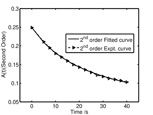
Again the two results are in close agreement. The graph of the experimental curve and the one that derives from our optimization method in given in Fig.(3).

Figure 3: Graph of the experimental and calculated curve based on the current induced parameter-dependent optimization method.

4 Conclusions

The results presented here show that for linked variables, it is possible to derive all the parameters associated with a curve by considering only one independent variable which serves as a function of all the other variables in the optimization process that uses experimental dataset as input variables in the estimation. Apart from possible reduced errors in the computations, there might also be a more accurate way of deriving parameters that are more determined by the value of one parameter (such as $k$ here) than others; the current methods that gives equal weight to all the variables might in some cases lead to results that would be considered "unphysical".

5 Acknowledgments

This work was supported by University of Malaya Grant UMRG(RG077/09AFR) and Malaysian Government grant FRGS(FP084/2010A).

References

- [1] J. J. Houser. Estimation of in reaction-rate studies. J. Chem. Educ., 59(9):776–777, 1982.
- [2] P. Moore. Analysis of kinetic data for a first-order reaction with unknown initial and final readings by the method of non-linear least squares . J. Chem. Soc., Faraday Trans. I, 68:1890–1893, 1972.
- [3] W. E. Wentworth. Rigorous least squares adjustment . application to some non-linear equations,I. J. Chem. Educ., 42(2):96–103, 1965.
- [4] W. E. Wentworth. Rigorous least squares adjustment . application to some non-linear equations,II. J. Chem. Educ., 42(3):162–167, 1965.
- [5] C. G. Jesudason. The form of the rate constant for elementary reactions at equilibrium from md: framework and proposals for thermokinetics. J. Math . Chem, 43:976–1023, 2008.
- [6] Mohammad Niyaz Khan. MICELLAR CATALYSIS, volume 133 of Surfactant Science Series. Taylor & Francis, Boca Raton, 2007. Series Editor Arthur T. Hubbard.
- [7] T. W. Newton and F. B. Baker. The kinetis of the reaction between plutonium(VI) and iron(II). J. Phys. Chem, 67:1425–1432, 1963.
- [8] J. H. Espenson. Chemical Kinetics and Reaction Mechanisms, volume 102(19). McGraw-Hill Book co., Singapore, second international edition, 1995.
- [9] W.H. Press, S.A. Teukolsky, W.T. Vetterling, and B.P. Flannery. Numerical Recipes in C -The Art of Scientific Computing . Cambridge University Press, second edition, 2002.