Giant QCD -factors beyond NLO
Abstract
Hadronic observables in Z+jet events can be subject to large NLO corrections at TeV scales, with -factors that even reach values of order 50 in some cases. We develop a method, LoopSim, by which approximate NNLO predictions can be obtained for such observables, supplementing NLO Z+jet and NLO Z+2-jet results with a unitarity-based approximation for missing higher loop terms. We first test the method against known NNLO results for Drell-Yan lepton spectra. We then show our approximate NNLO results for the Z+jet observables. Finally we examine whether the LoopSim method can provide useful information even in cases without giant -factors, with results for observables in dijet events that can be compared to early LHC data.
1 Introduction
At CERN’s Large Hadron Collider (LHC), it is widely anticipated that signals of new physics, for example supersymmetry, may manifest themselves as large excesses of data compared to expected QCD and electroweak backgrounds at high momentum scales [1, 2, 3, 4, 5, 6, 7]. The estimation of these backgrounds will be one of the elements in ascertaining the presence of any new physics from such signals. Consequently, considerable effort is being invested across the particle physics community in the development of methods to understand and predict backgrounds (some of the issues involved are described nicely in ref. [8]).
Given the QCD methods that are available today, some of the best prospects for obtaining systematic, accurate predictions of backgrounds involve next-to-leading order (NLO) QCD calculations. By carrying out a systematic expansion in the strong coupling and obtaining the first two terms (leading order (LO) and NLO) for a given process, one often obtains predictions that are accurate to . The importance of NLO predictions in the LHC programme has motivated a large calculational effort destined to extend the range of processes known at NLO (for reviews, see refs. [9, 10]).
While the majority of NLO calculations show some degree of convergence relative to the LO results, several groups have commented in recent years on the appearance of factors, ratios of NLO to LO results, that grow dramatically towards high transverse momenta [11, 12, 13, 14, 15, 16] (similar behaviour is visible also in [17, 18]). The problem generally occurs for hadronic observables (jet transverse momenta, etc.) in processes that involve heavy vector bosons or heavy quarks, at scales far above the boson or quark mass.
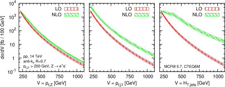
Fig. 1 illustrates this for the Z+jet process at LHC () energies. It shows the distributions of three observables that are non-zero for configurations involving a Z-boson and one or more partons: the transverse-momentum of the Z-boson (), the transverse-momentum of the highest- jet () and the effective mass (scalar sum of the transverse momenta) of all jets (). At LO, all three distributions are identical. At NLO, the observable is rather typical of a QCD observable: its distribution has a NLO -factor of about , fairly independently of , and its scale dependence is reduced with respect to LO. The distribution is more unusual: at high it has a -factor that grows noticeably with , reaching values of about , which is anomalously large for a QCD correction. The observable is even more striking, with -factors approaching .

(A)

(B)

(C)
Given that fig. 1 involves momentum scales where , one is driven to ask how it is that such “giant” -factors can arise. As touched on in [13], and discussed in more detail in [14, 15] for the case, the answer lies in the appearance of diagrams with new kinematic topologies at NLO. This is illustrated in fig. 2: at LO the only event topology (A) is that of a Z-boson recoiling against a quark or gluon jet. One type of NLO diagram involves gluon radiation from this basic topology, giving modest corrections to all our observables. However, there are also NLO diagrams (B,C) whose topology is that of a dijet event, in which a soft or collinear Z-boson is radiated from outgoing or incoming legs. These diagrams do not contribute significantly to the distribution, because the Z-boson carries only a moderate fraction of the total . However when examining , it is irrelevant whether the Z boson is soft or not. Contributions B and C then lead to a result that is of order , where the double logarithm comes from the integration over soft and collinear divergences for Z emission. The ratio of the NLO to LO results is therefore ,111This differs from double electroweak (EW) logarithms, which involve terms like , and are usually much smaller. Examples do exist of “giant” EW effects when tagging flavour [21]. rather than just , hence the -factor that grows large with increasing .222Part of the enhancement at high also comes from the fact that one can have scattering that emits a Z, whereas the partonic channel does not contribute at LO. For the observable the enhancement is even bigger because the dijet topology leads to instead of at LO.
While it is reassuring that we can understand the physical origins of the large -factors in fig. 1, we are still left with doubts as to the accuracy of the NLO Z+jet predictions for and , since they are dominated by the LO result for the Z+2-parton topologies. One way forward would be to calculate the full NNLO corrections for the Z+jet process. However, while work is progressing on NNLO calculations of processes with QCD final states (see e.g. [22] and references therein), results are not yet available; nor are they likely to become available any time soon for some of the more complex processes where giant -factors have been observed (e.g. some observables in [13, 17]). Alternatively one could simply try to avoid observables like and in inclusive event samples. For example, with additional cuts on the vector-boson momentum or a second jet, refs. [13, 15] showed that the -factors are significantly reduced. However, given the many analyses that are foreseen at the LHC, it is likely that at least a few will end up probing regions where giant -factors are present.
To understand how else one might address the problem of giant -factors, one can observe that in our example, the bottleneck in obtaining a NNLO prediction is the inclusion of the two-loop contributions and proper cancellation of all infrared and collinear divergences. Yet the two-loop (and squared one-loop) contribution will have the topology of diagram A in fig. 2 and should not be responsible for the dominant part of the NNLO correction, which will instead come from diagrams with the topology of B and C, with either an extra QCD emission or a loop. So if one includes tree-level and 1-loop diagrams (i.e. at NLO) and supplements them with even a crude approximation to the two-loop result, one that suffices merely to cancel all divergences, then one should have a good approximation to the full NNLO result (a related observation has been exploited to obtain approximate NNLO results for high- J/ production in [23]).
The purpose of this article is to develop a general method for obtaining such rough estimates of missing loop corrections. Our approach, called LoopSim, will be based on unitarity. After explaining how it works in section 2, and outlining a secondary “reference-observable” approach for control purposes, we will test the method by comparing its results to full NNLO predictions for lepton- spectra in Drell-Yan production in section 4, apply it to our Z+jet observables in section 5 and finally, in section 6, examine whether it can be of use even in the absence of giant -factors, specifically for a number of dijet observables.
2 The LoopSim method
The main ingredient of the LoopSim method is a procedure for taking a tree-level event with final state particles and supplementing it with a series of events with particles (approximate 1-loop events), particles (approximate 2-loop events), etc., such that the sum of the weights of the full set of events is zero. This “unitarity” property will ensure that all the soft and collinear divergences of the tree-level matrix elements will cancel against identical divergences in the simulated loop contributions.
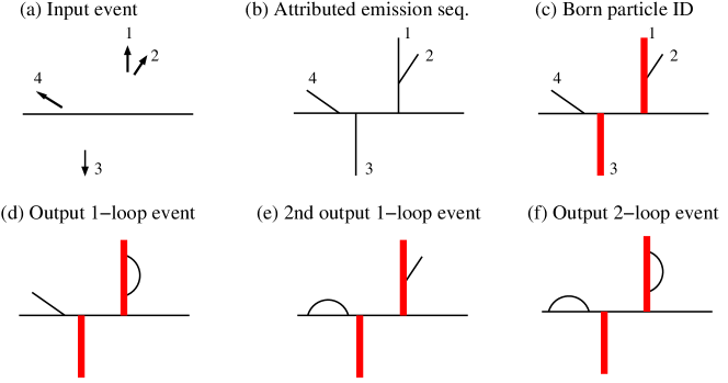
An outline of the procedure is given in fig. 3. Given a tree-level input event (a), the first step is to interpret it as a sequence of emissions (as if it had been produced by a parton shower), so that for example (diagram b) one can view particle 2 as having been emitted from particle 1, and particle 4 as emitted from the beam. The attribution of an emission sequence can be performed with the help of a suitable sequential-recombination jet algorithm and will be most meaningful in the limit that emissions are strongly ordered in angle and energy. The next stage is to decide which particles reflect the underlying hard structure of the event. If the event structure at the lowest possible order is that of a scattering, then one should identify two outgoing “Born” particles. The Born particles will remain present in all the approximate “loop” events that are generated. They are represented as thick red lines in diagram (c). Again this step is most meaningful when all non-Born emissions are soft and collinear.
One then generates a set of simulated “1-loop” events by finding all ways of recombining one emitted particle with its emitter, diagrams (d,e). Each such “1-loop” event comes with a relative weight of compared to the tree-level diagram. Similarly the set of simulated “2-loop” events is obtained by finding all ways of recombining two emitted particles with their emitter(s) (diagram f), each with relative weight ; and so forth down to events where only Born particles remain (in fig. 3 this is already reached at the two-loop level). Note that the loop-diagrams drawn in fig. 3 are not intended to represent the actual Feynman diagrams that would be relevant at 1 and 2-loop level. Instead they indicate the way in which we have approximated the loop divergences, as the unitarising counterparts of the divergences that appear for each emission in the soft and collinear limits.
Given the above procedure for unitarising tree-level events, we shall see that it is then straightforward to extend it to event sets that also include exact loop diagrams.
2.1 The tree-level pure glue case
We start by examining the LoopSim procedure in the simple case of purely gluonic tree-level events. This will suffice to introduce most of the relevant concepts. Section 2.2 will then discuss some of the additional issues that arise for events with quarks and vector bosons, while the handling of events sets that include exact loop diagrams will be left to section 2.3.
It is helpful to introduce some notation: Firstly, is the number of final-state particles present in the lowest relevant order (i.e. the number of final-state “Born” particles). For instance if considering higher-order corrections to dijet events, as in fig. 3. represents a generic event with final state particles. So the starting event of fig. 3 would be labelled . Finally, will be an operator that acts on an event and returns all the events at loops obtained from using the LoopSim method. For instance, fig. 3d,e represents the action of on the input event (a).
The central part of the LoopSim method involves the construction of the operator acting on for all ( because the number of real final state particles cannot be smaller than that of the lowest order event).
2.1.1 Attribution of structure to events
Recall that the primary function of the LoopSim method is to cancel the divergences that appear in the soft and collinear limits. In these limits, events can be interpreted as stemming from a sequence of probabilistic (parton-shower) type splittings of some original hard Born particles. The knowledge of the splitting structure will help us generate loop events to cancel the divergences.
The attribution of a branching sequence is most easily performed using a sequential recombination jet algorithm (and is inspired by the CKKW matching procedure [24]). We will use the Cambridge/Aachen (C/A) algorithm [25, 26], which has important advantages over the algorithm when dealing with nested collinear divergences (avoiding “junk” jets [25]).333All jet clustering in this article is carried out using FastJet [27, 28].
As a first step, to each of the particles in the event , we assign a unique “identity” index .
We then run the Cambridge/Aachen (C/A) algorithm on the event. It repeatedly clusters the pair of particles that are closest in angle, i.e. with smallest where is the usual squared angular distance in the plane, and is a free parameter, the LoopSim radius. The C/A algorithm continues until all the , at which point the remaining particles are deemed to cluster with the beam.
An clustering in the C/A algorithm can be reinterpreted as a splitting. The C/A algorithm does not distinguish in any way between and . However, in the soft limit, say , rather than viewing as splitting to and , it is a better reflection of the divergent structure of the amplitude to view as having emitted a soft gluon . Then is nothing other than particle with some small fraction of its energy removed. To account for this, in an clustering, if , then we declare that the “identity” of particle should be the same as that of particle , . Also we record as being a “secondary emitter” and remember that the object with identity has been emitted from the object with identity . (Exchange if ). This is represented in fig. 3b by the fact that particle is a straight line, off which particle has been emitted; the identity of the combination is . For an clustering, we record as having been emitted from the beam.
The next step in attributing structure to the event is to decide which event particles should be viewed as the Born particles, i.e. which particles are responsible for the hard structure in the event. Inspired by the original formulation of the Cambridge algorithm [25], for every recombination we assign a algorithm type hardness measure [29, 30].444In the results shown later, we actually used , which however is identical for our default choice of . For every beam recombination, we assign a hardness .
We then work through the recombinations in order of decreasing hardness. For an recombination (or splitting), assuming is harder than , we mark as a Born particle. If fewer than particles have already been marked as Born particle, we also mark as a Born particle. For an recombination, we mark as a Born particle. This is repeated until particles have been marked as Born (a particle may be marked more than once; in such a case its marking counts only once). As an example, in fig. 3, the hardest recombination will be between particle and the beam, so particle is marked as a Born particle. The next hardest recombination will that of with the beam. Therefore we mark as a Born particle. This exhausts the number () of Born particles that need to be marked.
At the end of the above procedure, every particle will have been marked as emitted either from the beam or from another particle, and some particles will also have been marked as secondary emitters and/or Born particles. Thus in figure 3, particle is labelled as having been emitted from the beam, it is a secondary emitter and a Born particle; particle is labelled as having been emitted from particle ; particle is a Born particle, emitted from the beam; and particle was emitted from the beam. The structure that we attribute is of course physically unambiguous only in the presence of strong ordering of emission angles and energies. However, as we shall argue in section 2.4, the mistakes that we make for non-ordered configurations should have a small impact for observables with giant -factors.
2.1.2 Constructing virtual (loop) events
Once every particle is labelled in an event , one can compute the result of , which is a set of events . For an event with respectively Born particles and non-Born secondary emitters, we define
| (1) |
to be the maximum number of particles that will be allowed to become virtual in a given event. It is obvious that Born particles will not become virtual. Additionally, secondary emitters will also not become virtual. To understand why, consider the event
![[Uncaptioned image]](/html/1006.2144/assets/x6.png)
|
(2) |
in which particle is a secondary emitter, since it emitted . There is a divergence for to be collinear to only if is a final-state particle. If instead is made virtual, then the divergence for emitting no longer exists (there is no divergence for emission from internal lines in a diagram), so that the weight for the diagram in which is virtual would be the weight of the tree-level diagram times a small coefficient . This simplest way of accounting for this is to approximate and thus not generate events in which secondary emitters are made virtual (a more detailed discussion is given in appendix C).
Having understood which particles can be made virtual, the operator , when applied on an event , generates all the diagrams in which particles become virtual. For the virtual events to cancel the infrared and collinear divergences that appear in the tree-level diagram, we need an infrared and collinear (IRC) safe procedure to make particles virtual. For instance, the divergent weight of an event with two collinear partons and has to be cancelled by that of corresponding virtual event ( makes a loop over ) when computing the distribution of any IRC safe observable; and two collinear partons, if not virtualised, have to remain collinear when another particle becomes virtual.
There are two ways for a particle to make a loop:
-
•
If it is labelled as clustering with particle , then one has to spread the momentum of particle over and all the particles that are labelled as clustering with it but which were emitted after according to the C/A clustering sequence (i.e. at smaller angle). The exact procedure is explained in detail in appendix A, and is designed to ensure that the recombination maintains any collinearity properties of non-looped particles and is invariant under longitudinal boosts. When is the only particle that clusters with , then the procedure becomes equivalent to adding the momenta of particles and , , and then rescaling the momentum such that its mass is set to , while leaving its transverse components , and its rapidity unchanged.
-
•
If particle is labelled as clustering with the beam, then when it is “looped” it is simply removed from the event. Note that looping particles with the beam is less trivial than it may seem at first sight, because of an interplay with factorisation and the PDFs. Nevertheless it can be shown, appendix B, that for particle types that are included in the PDFs it does make sense to loop them. A imbalance will result from the looping of particles with the beam, and so after all loops have been made, we apply a transverse boosts to all remaining event particles, conserving their rapidities, so as to bring the total transverse momentum to zero (again, see appendix A).
There is some arbitrariness to our procedures for producing physical kinematics in the looped events. One avenue for future work would be to examine the impact of making different choices.
The operator has the following properties
| (3) |
If is the weight of event , then each of the events generated by the operator has a weight
| (4) |
Once all the have been calculated for , one has to combine them in order to subtract all the soft and collinear divergences that appear in the calculation of and the virtual diagrams generated from it. This is done by the operator , which is defined as
| (5) |
It generates all the necessary looped configurations that have the same order in as the original tree-level diagram. It is straightforward to see that the total weight of the diagrams obtained from the operator is . Indeed, if we apply it to an event whose maximum number of virtual particles is , we get
| (6) |
for .
We note that the above procedure for approximating loop diagrams does not generate the finite terms needed to cancel the scale-dependence of lower-order diagrams. While it would be straightforward to include such terms, we believe that in the absence of full loop calculations, not including them helps ensure that the standard procedure of variation of renormalisation and factorisation scales is more likely to provide some form of reasonable estimate of the uncertainties on our results.
2.1.3 Some examples
In order to illustrate the action of the operator , we give below some simple examples in the pure glue case. In each of these examples, only the Born particles are labelled with numbers
| (7a) | |||||
| (7b) | |||||
| (7c) | |||||
| (7d) | |||||
| (7e) | |||||
| (7f) | |||||
Eq. (7a) gives an example of singly-looped configurations (“1-loop diagrams”) generated by LoopSim when studying the contributions to QCD dijet production. Eq. (7b) shows the “2-loop diagrams” generated from the same event. The next equation shows what happens if we add one more particle to the final state. If, eq. (7d), we now set the number of Born particles for the same event to be , we obtain only one -loop diagram instead of three, as represented in eq. (7d).555One might reasonably be surprised by this: after all, the result for the exact two-loop diagrams is independent of any choice of number of Born particles. The point is that if one studies soft and collinear corrections to the 3-jet cross section, then for the events in eq. (7c) where the particle labelled in eq. (7d) is virtual, the event will resemble a two-jet event and so not pass the 3-jet cuts. However if one studies the 3-jet cross section in a kinematic region where the cuts allow one of the jets to be much softer than the others, then to obtain sensible results it becomes necessary to use and include all diagrams on the right-hand side of eq. (7c). Finally, the last two examples of eq. (7) give a case with a splitting: the emitter is not looped, even if it is not a Born particle.
We also give a few examples of the action of the operator:
| (8a) | |||||
| (8b) | |||||
| (8c) | |||||
In the last case, only one particle can become virtual because there are two secondary emitters which cannot be looped.
2.2 Treatment of flavour within LoopSim
Let us now examine some of the issues that arise if we are to extend the LoopSim method to processes with quarks and vector bosons.

We start with quarks and consider the situation depicted in fig. 4. In this case, applying the C/A algorithm as in the previous section will lead to the recombination of the two quarks and , which is clearly not physical. If flavour information is available for events, then one can veto on such a clustering, for instance by defining the clustering distance between two quarks to be infinite. As discussed in [31] such a modification alone is not sufficient to systematically guarantee sensible treatment of flavour in jet clustering. Refs. [31, 32] have both discussed the further modifications needed in the case of the algorithm. A proper handling of flavour within LoopSim might seek to extend those modifications to the C/A algorithm. However, neither of the NLO programs that we use, MCFM and NLOJet++, provide information on particle flavours, so we defer such modifications to future work and just maintain the distance for all partons. For observables that are not flavour-sensitive this should not be a major drawback, given the observation [31] that divergences associated with the mistreatment of flavour are strongly subleading. Were we to be interested in heavy tagged quarks, more careful treatment might well be needed. Note that there are also subtleties related to flavour and PDFs, discussed in appendix B.
What about non-QCD particles, specifically vector bosons? Let us examine the case of Z bosons. A Z can be emitted from quarks or antiquarks and we would like this to be reflected when establishing the approximate emission sequence, because if the Z has been emitted from a quark, then that quark is a secondary emitter and should not be looped. In other cases a Z boson may be the hardest isolated object in an event. Then it is to be considered a Born particle. On the other hand we won’t necessarily wish to consider diagrams where a Z boson is looped, because they would represent electroweak corrections, not QCD corrections.
One issue in dealing with electroweak particles is that they are not emitted from gluons. If one could distinguish between quarks and gluons, then this could be accounted for during the C/A clustering, by defining the distance between a Z and a gluon to be infinite. Since we will not know which partons are quarks or gluons, we adapt Frixione’s isolation procedure [33] to decide if a Z boson relatively close in angle to a parton is likely to have been emitted from . More precisely, if
| (9) |
then we define , otherwise . When recombining and Z into a particle , then the identity index is set equal to (a quark and a Z give a quark). Our procedure means that a Z that is very collinear to a parton is always considered to be emitted from that parton — this makes sense because such configurations are much more likely to occur when the parton is a quark. In contrast a soft parton in the general vicinity of a Z is not clustered with the Z, which is sensible given that most soft partons tend to be gluons. Finally, for a recombination between a parton and Z, we define the hardness of the branching as666This will be true in a future version of the code, but currently .
| (10) |
while a recombination of a Z with the beam has a hardness
| (11) |
The latter means that for an event with just a parton and a recoiling Z boson, the parton’s beam hardness will always be lower than the Z’s, implying that for it is the Z-boson that will be the single Born particle, as should be the case, at least when the parton has , i.e. in the kinematic regime that dominates the total cross section for the Z.
Once a structure has been assigned to an event with a Z boson, the next question is that of the looping procedure. When looping partons it remains identical to before, with just a small extension of the recoil procedure in order to deal with decay products of the Z boson (see appendix A). In the situations where the Z is not a Born particle (it is never an emitter), straightforwardly following the procedure of section 2.1.2, one would deduce that one should loop the Z as well:
| (12) |
(straight lines are partons, either quarks or gluons). The rightmost diagram, with the looped Z, is not, however, a QCD loop diagram: it is an electroweak loop correction to a multijet event. The LoopSim procedure does not aim to reproduce electroweak loop corrections (though in this case it might be a reasonable approximation). Furthermore, in any analysis that tags on Z bosons, such a diagram would not be tagged and so would not contribute. Thus, although the LoopSim procedure naturally generates events with looped Z bosons, events like the rightmost diagram of eq. (12) are simply to be discarded.
For events with bosons, the same procedure can be used as for Z’s. Note, however, that while the “looped” Z events may give a reasonable approximation to actual electroweak loop diagrams, looped events will not. This is because -boson emission changes quark flavour: consider a tree-level diagram , with the emitted collinearly off the incoming , converting it into a . The LoopSim procedure would give a “loop” diagram , with the looped. However no such loop diagram exists and the correct loop diagram would instead involve .777A similar problem would appear to exist with the QCD diagram , with the incoming gluon splitting collinearly to give , and the outgoing collinear being looped. Here, however, we are saved by the interplay between LoopSim and PDFs, as discussed in appendix B. It is crucial in this respect that all flavours that get looped are included in the PDFs. This is closely related to the phenomenon of Bloch-Nordsieck violation [34] that is found when considering electroweak double logarithms. Since we in any case discard events in which electroweak bosons are looped, this should not be a problem for the practical use of LoopSim in events with bosons.
2.3 Merging NLO calculations and beyond
Before explaining how we merge exact higher orders calculations, let us mention how we use the LoopSim method in practice on tree-level events at several different orders. We introduce the notation X@pLO to denote an approximation to the NpLO cross section for producing X, with all loop terms estimated through the LoopSim procedure. It is obtained by applying the operator to all tree-level diagrams that can contribute up to NpLO. For instance, one can write
| Z@LO | (13a) | |||
| Z+j@LO | (13b) | |||
| Z+j@LO | (13c) | |||
Notice that and . The terms and simulate up to one-loop corrections, and simulates up to two-loop corrections.
Now let us see how things work beyond tree-level accuracy. We define to be a generic event at loops (exactly calculated) with particles in the final state. We first consider the case where only one-loop corrections are computed exactly, so that we have tree-level events and exact one-loop events . As before we can apply the unitarisation operator to the tree-level events, . However, since we now include exact 1-loop contributions, , we must remove the approximate 1-loop contributions that are contained in . This alone is not sufficient, because among the extra contributions from the exact 1-loop terms, there will be pieces that are finite for a given -parton configuration, but that can lead to divergences when integrated over the -parton phase space. To cancel these extra divergences, we should introduce additional approximate higher-loop contributions, which can be obtained by applying the unitarisation operator to the difference between the exact and approximate one-loop terms. So, rather than including just events and subtracting , we include events and subtract . It is convenient to express this through a new operator such that
| (14a) | ||||
| (14b) | ||||
where the extra subscript on the indicates that it is the form to use when the exact 1-loop result is to be included. The action of depends on the number of loops already included in the event on which it operates: we subtract the one-loop contribution returned by LoopSim only in tree-level events. With this notation, one can compute the higher order corrections to eqs. (13) to one-loop accuracy,
| Z@NLO | (15a) | |||
| Z+j@NLO | (15b) | |||
| Z+j@NLO | (15c) | |||
where the “only” subscript on Z+j@NLO means that we take the highest order that contributes, i.e. here , since the LO, , piece of Z+j@NLO, is already taken into account in the Z+j@NLO contribution. This implies that one should use consistent renormalisation and factorisation scale choices across all different orders of the calculation. Note that in eq. (15) we have introduced the notation pNqLO to denote an approximation to the Np+qLO result in which the highest loop contributions have been approximated with LoopSim.
The extension of the procedure beyond one-loop accuracy is simple. For instance, at two-loop accuracy, one has to subtract the approximated two-loop contribution in eq. (14a), and the other approximated two-loop contribution in eq. (14b), giving
| (16a) | ||||
| (16b) | ||||
| (16c) | ||||
Therefore, once Z+j@NNLO is calculated, one may compute for instance
| (17) |
To be complete, let us mention the generalisation of our procedure to -loop accuracy
| (18) |
We noted at the end of section 2.1.2 that the plain LoopSim procedure does not generate the finite terms needed to cancel residual scale dependence from lower orders. With the introduction of the exact loop contributions, those finite terms do now get included. Thus for a given number of exact plus simulated loops, as we increase the number of exact loops, we should expect to see reductions in scale uncertainties.
2.4 Expected precision of the method
Let us briefly explain why the LoopSim method is expected to work in the presence of giant -factors. We consider an observable computed respectively at NLO and LO. We define such that
| (19) |
and we assume that . This huge -factor may come from logarithmic enhancements in the real NLO diagram or the appearance of new scattering channels in the perturbative expansion. The computation of gives the exact real part of the NLO calculation as well as the divergent terms of the virtual correction. Therefore
| (20) |
where, in writing , we mean that the term missing in the LO calculation, the finite part of the 1-loop correction, is not especially enhanced. This leads to
| (21) |
The relative difference between the approximate and exact NLO calculations is thus suppressed by the inverse -factor.
Next, consider NLO accuracy. The difference between and comes from the parts of the two-loop corrections that are finite and associated with the LO topology, so that they should be free of the enhancements that led to the large NLO -factor. This implies
| (22) |
If we define such that , then we can write
| (23) |
If , one can expect too.
3 The reference-observable method
Given the novelty of the LoopSim method, it is useful to have an alternative way of estimating the size of the NNLO contributions that we will approximate with LoopSim. Here we outline such an alternative method, which, though less flexible than the LoopSim approach, will provide a valuable cross-check and help us build our confidence in results of the LoopSim method.
Let us explain it for observables in the Z+j process. Our aim is to estimate for some observable .888More precisely, is the cross section for the observable to pass some given cuts; it is only for brevity that we use here the somewhat inaccurate shorthand “cross section for observable ”. We assume that we have a reference observable which is identical to the observable at LO. For instance, one might consider and . We can write the NNLO Z+j prediction for in terms of the NNLO prediction for the reference observable plus the NLO Z+2j difference between and the reference cross section
| (24a) | ||||
| (24b) | ||||
The second equality is possible because 2-loop NNLO corrections to Z+j have the topology of Z+j at LO. Therefore, their contributions to the observables and ref are identical and cancel in the difference in eq. (24a).
If we have reason to believe that the perturbative expansion for the reference observable converges well, we can conclude that is genuinely a small correction. Then
| (25) |
i.e. we approximate the NNLO distribution for in terms of the NLO distribution for the observable and a NLO calculation for difference between the and distributions, both of which are exactly calculable. The missing part is suppressed by a relative factor , as for the LoopSim method. For Z+j, one can see from fig. 1 that seems to be an acceptable reference observable for and .
In the sections that follow we shall, for brevity, refer to the RHS of eq. (25) as “ref. NLO” even though it does not quite adhere to our the meaning of NLO as set out in section 2, i.e. in terms of the specific sets of tree-level and loop diagrams that are included exactly.
4 Validation: comparison to DY at NNLO
The cross section for the Drell-Yan process is known with exclusive final states up to NNLO accuracy [35, 36]. Above a certain value of lepton transverse momentum, one finds giant corrections to the lepton spectra when going from LO to NLO and large ones from NLO to NNLO. This gives us an opportunity to directly test the performance of the LoopSim method by comparing its NLO results to exact NNLO spectra for lepton pair production.
Before examining NLO results, it is useful to compare LO with NLO. If they are in reasonable agreement for some observable, then that serves as a first indication that the LoopSim estimate of missing loop corrections is sensible for that observable.
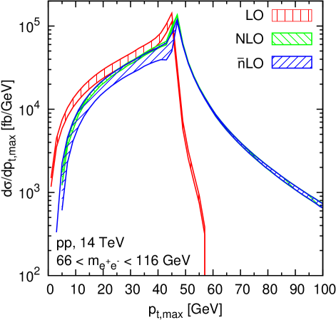
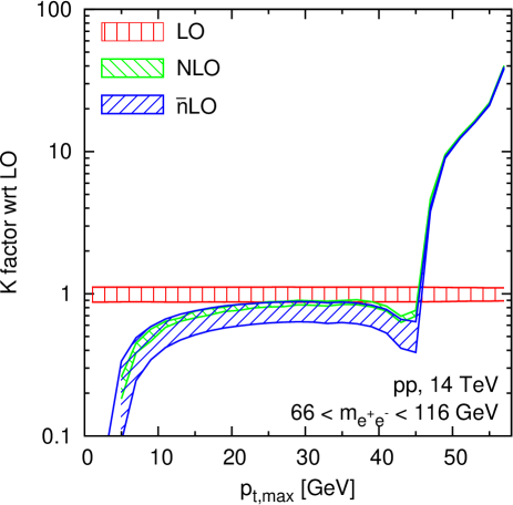
Fig. 5 gives the comparison of the LO, NLO and LO results for the production of an pair within the mass window of GeV at a proton-proton centre of mass energy of TeV. The left-hand plot shows the cross section differential in the transverse momentum of the harder of the two leptons. The right-hand plot gives the corresponding K factor with respect to LO. The results were obtained with MCFM 5.3 [37, 19], with its default set of electroweak parameters and NNLO MSTW2008 parton distribution functions. The uncertainty bands in Fig. 5 correspond to varying the renormalisation and factorisation scales by a factor of and around a default choice of . In the LO result we fixed the value of the LoopSim radius parameter to be , which naturally places interparticle and particle-beam clustering on the same footing (though the LO result here is actually independent of , because there is at most one isolated QCD parton in the final state).
There are three relevant regions of transverse momentum in fig. 5. For (low ) the distribution is dominated by on-shell Z-bosons and its shape is governed by the angular distribution of the Z decays in their centre-of-mass frame. The peak close to corresponds to Z-bosons that decay in a plane at right-angles to the beam. For (intermediate ), the LO distribution comes from Z-bosons that are off shell, which allows the of the lepton to be larger than . The narrow width of the Z causes the distribution to fall very steeply. The upper edge of this region is a consequence of our cut on . Above (high ) the LO distribution is zero.
In the low region, the NLO correction is moderate and negative. There is no strong reason to believe that the LoopSim method should work here, but it turns out that the LO result reproduces the structure of the correction, even if its scale dependence remains much larger than that of the NLO result (this is because the LoopSim procedure does not include the finite terms that would partially cancel the LO scale dependence). In the intermediate region, we see a “giant” NLO -factor. It comes about because initial-state radiation can give a boost to the Z-boson, causing one of the leptons to shift to higher (it becomes the “max” lepton). The spectrum of QCD radiation falls much less steeply than the Z-boson lineshape, so this NLO correction dominates over the LO result. In this region the exact loop correction, proportional to the LO result, becomes almost irrelevant and we see near perfect agreement between LO and NLO. In the high- region only the real emission diagrams of Z@NLO contribute and LO becomes identical to NLO (both correspond to the Z+j@LO result). Similar results hold for the distribution, while the lacks the giant -factor in the intermediate region.
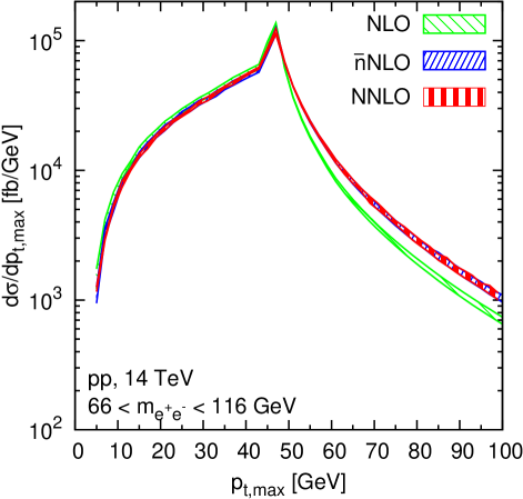
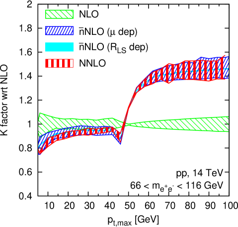
A similar comparison between NLO and NNLO spectra is shown in fig. 6. The NNLO results were obtained with DYNNLO 1.0 [36, 38, 39], used with a set of electroweak parameters compatible with that of MCFM.999 In its and contributions, DYNNLO includes among its parameters a cut on the of the Z boson. The cut is applied to both real and virtual terms and its impact should vanish as it is taken towards zero. It is, however, required to be non-zero for the numerical stability of the MCFM Z+j NLO calculation that is among the components of DYNNLO. We set the cut equal to in the term and to in the term. A related cut was placed on the piece of the NLO result (while none was used at ). The impact of the cut is small but not entirely negligible close to the peak (where, physically, NNLO should in any case be supplemented with a resummation).
In the low- region we find quite good agreement between the NLO and NNLO results (with somewhat larger uncertainty bands for NLO). Such a result was not guaranteed a priori, even if it is not entirely surprising given the reasonable agreement that we saw between LO and NLO. In the intermediate region, where the NNLO/NLO corrections are substantial, the agreement is excellent. This was expected. At high the agreement should be exact, and does seem to be, within statistical fluctuations. The dependence on (shown in the right-hand plot) has been estimated by varying its value from 0.5 to 1.5. The effects are small.
Finally, we note that similar features and a similar level of agreement between NLO and NNLO are to be found in the and distributions.
5 Results for the jet process
In the previous section, we studied the Z production process and showed that our procedure correctly reproduces the distribution of the hardest lepton at NNLO, even, unexpectedly, in regions where the -factor is not large. In this section we study the Z+j process, whose NNLO cross-section is not known yet, but which leads to giant -factors at NLO for some observables as explained in the introduction. Therefore, their NNLO contributions are expected to be accurately described by the LoopSim method. Throughout this section we use MCFM 5.7, including the Z+2j process at NLO [40], with the NLO CTEQ6M PDFs. We will take three different values for the renormalisation and factorisation scales: , and , with
| (26) |
where is the transverse momentum of the hardest jet. At high , this scale choice should be quite similar to that used in [41] and has the same scaling as those in [14, 15]. The uncertainty is measured at using three different values for it: , , .
In addition to the 3 observables shown in the introduction, , and , we will also consider
| (27) |
We only include events for which .
5.1 Validation at LO
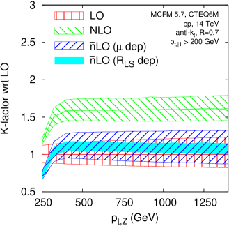
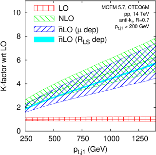
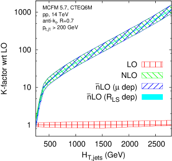
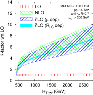
As a first investigation of the performance of the LoopSim method, let us examine how the LO approximation compares to the full NLO result. Fig. 7 shows the -factors for the LO and NLO predictions, with uncertainty bands from scale and variations.
In the upper-left plot, one sees that the LO prediction for the distribution gives a somewhat smaller -factor than the NLO result. We interpret this as being because certain genuine loop effects are not taken into account by the LoopSim method, for example those related to threshold logarithms, which depend crucially on the factorisation scheme of the parton distribution functions. The LO result does, however, reproduce the dependence of the -factor, i.e. the dip towards . This dip arises because of the requirement in our event selection that there should be at least one jet with . At LO this induces a step-function in the distribution at . At NLO, soft and collinear emissions smoothen out that threshold and the LO calculation correctly reproduces the resulting interplay between real and virtual terms.
In the three remaining plots of fig. 7, for , and , all of which have giant -factors, one sees good agreement between the LO and NLO results. This is because the dominant NLO contribution comes from events in the B and C-type configurations of fig. 2, for which there is no corresponding QCD loop correction. The LoopSim method merely serves to cancel the divergences that arise from soft and collinear emissions off -type configurations and these are not dominant overall.
The dependence, also shown on these four plots, only comes from -loop events generated by LoopSim. Therefore, for an observable studied in Z+j@LO with two different values and for , one can write:
| (28) |
as long as coincides with at LO (it does for each of , and ). This means that the absolute uncertainty due to is the same for and . Therefore, the relative uncertainty due to is expected to be roughly inversely proportional to the -factor for , in analogy with the discussion of sec. 2.4. This explains why the dependence (solid cyan band) looks significantly smaller for , and than it does for plot.
5.2 Results at NLO
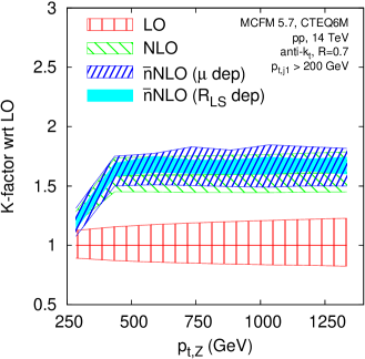
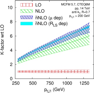
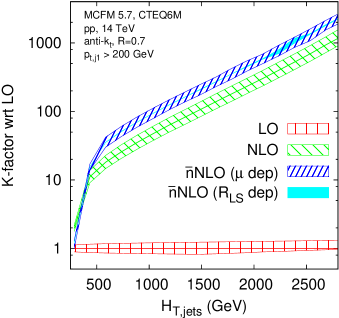
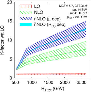
Results at NLO are given in fig. 8. In the case of the result is similar to the NLO result, and the scale uncertainties remain largely unchanged. In other words, since Z+2j topologies do not dominate the high- distribution, adding NLO corrections to them (i.e. NLO Z+j) makes no difference either to the result or to the uncertainties. We have also shown the dependence on the choice of in the LoopSim procedure. It is smaller than the scale dependence.
The distribution gets a correction that is just within the NLO uncertainty band, with NLO uncertainties that are about half the size of the NLO band. Adding in the NLO term has made a real difference. This is precisely what we expect: the observable is dominated by Z+2-parton configurations, and these were only present at tree-level in the NLO Z+j calculation. Our use of NLO provides the additional 1-loop Z+2-parton and tree-level Z+3-parton configurations that come with NLO Z+2j accuracy.
Given the improvement in scale uncertainty, we need to ask whether the uncertainty due to variation might somehow eliminate part of this benefit. It is, however, small. The reasons are similar to those given around eq. (28).
The and distributions get significant NLO corrections, with NLO/NLO -factors of about . Absolute scale uncertainties increase slightly compared to NLO, but because of the large -factor, relative scale uncertainties diminish. At first sight, it is somewhat disturbing that the NLO and NLO uncertainty bands don’t overlap. Given the novelty of the LoopSim method, one should therefore ask whether this is reasonable and whether there is any way of cross-checking the result.
A first observation is that since NLO Z+j is really NLO of the dominant Z+2j component, the large NLO corrections that we see are comparable to an -factor for going from LO to NLO in the Z+2j prediction. There are many contexts where NLO and LO results are not compatible within scale uncertainties, and so it is not unreasonable that the same should be seen here.
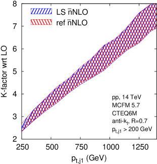
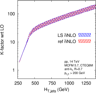
Still, we would like to have some more quantitative cross checks that our results are sensible. One option is to consider the alternative “reference-observable” method presented in section 3, which only makes use of standard NLO calculations to compute the approximate NNLO corrections. The comparison between the two methods is shown in fig. 9 for and , where we have taken as the reference observable. One notices near perfect agreement for and very good agreement for . This gives us some degree of confidence that the NLO LoopSim results provide an accurate description of the NNLO behaviour for these observables.
A second option for cross-checking the large NLO effects for and , is to examine whether type observables might generally be “difficult”. To do so we look at them in the case of QCD jet events.
6 QCD jet events as a testing ground
We have seen that the NLO -factors for the two effective-mass variables, and , in jet(s) events are about a factor of two above the NLO -factor.
Since NLO is the first order at which we see the dominant “dijet” topology for the variables in Z+jet(s), fig. 2B,C, it might be instructive to establish a correspondence with a simpler process, QCD dijet production. Having a NLO Z+j prediction is analogous to a LO dijet prediction; and the NLO Z+j predictions should be analogous to NLO dijet predictions. NLO cross sections for dijet observables can be calculated exactly and therefore we can check whether NLO -factors of order appear for effective-mass observables in pure QCD events.
We will consider several effective-mass observables: an variable, which sums over the hardest jets above some threshold (; such a cut is often imposed experimentally101010In section 5 we did not apply this kind of cut on the variables; one purpose in applying it here is to ascertain whether the large higher-order effects persist even with it.)
| (29) |
where is the transverse momentum of the hardest jet. Upper limits on the number of jets included in the effective mass are common in SUSY searches [3, 4]. We also define an effective mass for all jets above the threshold,
| (30) |
which is similar to the and observables of section 5. Finally, for completeness we will consider the distributions of , and the inclusive jet spectrum. All our results in this section will be for a centre-of-mass energy of , to allow comparison to results in the current run of the LHC.
At LO, the distributions of (), , , and will all be identical. The inclusive jet spectrum will have a distribution that is twice as large (because each of the two jets contributes). Note that we do not impose any rapidity acceptance limits on the jets: though such a cut would have been trivial to include in the LoopSim procedure, it would have complicated somewhat the reference-observable approach that we will consider at the end of the section. LoopSim results with a rapidity cuts of on the jets are available from the authors on request.
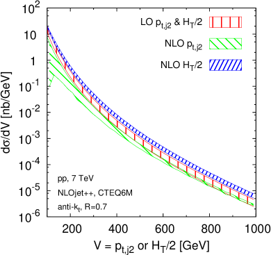
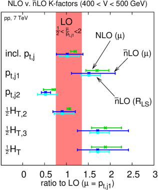
Figure 10(left) shows the distributions for two observables, and at LO (where they are identical) and at NLO, as determined using NLOJet++ [42, 43] with CTEQ6M PDFs. A first comment is that receives a NLO -factor of order , just like the NLO enhancements in the Z+j case. This provides supporting evidence as to their legitimacy. A second comment is that the cross sections are large: these observables will be easily accessible with a few pb-1 of integrated luminosity at a LHC, allowing for an early experimental verification of the large -factor for .
The other observable in the left-hand plot of fig. 10, , has a very different -factor, somewhat below . The right-hand plot shows the NLO -factors for our full range of observables, focusing on a single bin of the left-hand one, from . The pattern that we see here allows us to make some deductions. Firstly, the variable, which sums the ’s of the two leading jets, is free of large NLO enhancements. It is the addition of the third jet in and that brings about the enhancement. A natural interpretation is the following: it is common for a third, soft jet to be present due to initial state radiation. This third jet shifts the distribution to slightly larger values, and because the distribution falls very steeply, that leads to a non-negligible enhancement. This suggests that if, in section 5, we had used effective mass observables with at most two objects in the sum, then the NLO/NLO ratios would have been close to . We have verified that this is indeed the case.
The pattern for and in fig. 10 can also be explained in similar terms: a soft ISR emission boosts the hard dijet system, breaking the degeneracy between the ’s of the two hardest jets. It is jet that shifts to larger (giving a -factor ), while jet shifts to lower and so it gets a factor below . For the inclusive jet spectrum, and for , this effect balances out. In addition, final-state radiation from one of the jets can cause it to shift to lower (becoming the 2nd jet), further reducing the -factor for the distribution of .
Of the different variables, it is only the inclusive jet and for which there is a clear reduction in scale uncertainty in going from LO to NLO.
Figure 10(right) also shows the LO results (including uncertainties both from scale variation and from the LoopSim parameter ). Despite the fact that none of the -factors is parametrically large (except arguably for and ), the LO results are remarkably effective at reproducing the pattern of NLO -factors, albeit with a small systematic shift and generally larger scale uncertainties. One can also verify that, to within , the dependence of the NLO -factors is reproduced at LO.
Given this success of LO, and the observed limited convergence of some of the observables at NLO, it is interesting to examine what happens at NLO, where the additional 3j@NLO contribution that we require is again obtained using NLOJet++. Results are shown in fig. 11.
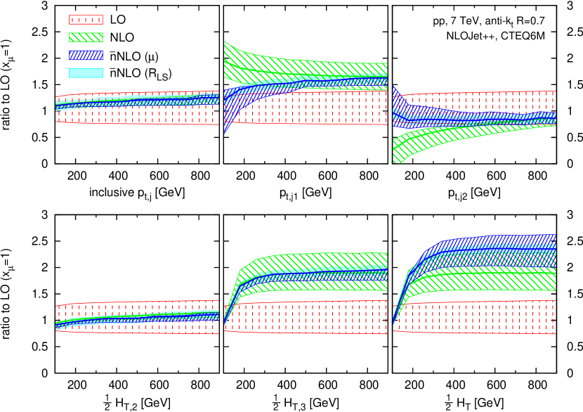
For the inclusive jet spectrum and , which already saw large reductions in scale-dependence at NLO, the NLO corrections have essentially no meaningful effect: they neither significantly affect the central values, nor reduce the scale uncertainties. For these observables, NLO already converged well, and adding a subset of the NNLO corrections without the 2-loop part cannot improve the result.
For the other effective mass observables, the situation is quite different. With , the NLO result is close to the NLO result and the scale uncertainty is much reduced, i.e. this observable seems to come under control at NLO. In contrast, is subject to quite a large further correction, with the central value at NLO lying outside the NLO uncertainty band, and the NLO uncertainty band (dominated by scale variation) only marginally smaller than at NLO. Why is this? Perhaps we are seeing the effect of a second ISR emission, which shifts the distribution to even higher values? Given that converges and does not, such an explanation is not unattractive. It is also consistent with the decrease in -factor at low , where the cutoff on the jets contributing to the sum will eliminate the ISR enhancement. A definitive conclusion would however probably require further study.
For the remaining two observables, and , the NLO contribution goes in the opposite direction from the NLO correction and at low it seems that the series fails to converge. This is, we believe, closely related to observations of insufficiencies of NLO predictions for dijet cross sections in DIS and photoproduction when identical cuts are imposed on both jets [44, 45, 46, 47, 48] (equivalent to integrating the distribution above that cut). The worse convergence at low is probably due to the larger fraction of subprocesses that involve gluons in the underlying scattering, so that perturbative corrections tend to go as rather than as at higher .
Considering that we do not have giant NLO -factors for the jet processes shown here, one may question the validity of the information obtained from the LoopSim procedure. An important cross check comes from a comparison with the reference-observable technique. Examining fig. 10 (right), one sees two natural reference observables: the inclusive jet spectrum and , both of which show “perturbative” -factors and small scale dependence at NLO. Here we will use (half) the inclusive jet spectrum as the reference observable (results with would be almost identical).
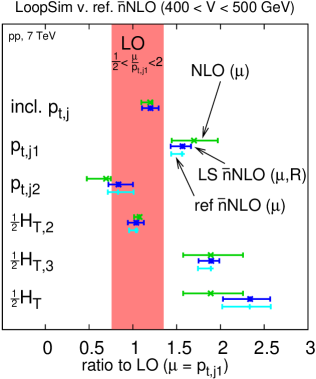
Figure 12 provides a comparison of the LoopSim NLO results (showing the envelope of the scale and uncertainties) with the reference-observable NLO results. The comparison is given for all observables except the reference observable itself. The agreement between the two methods is striking, with the reference-observable method giving just a small shift of the -factors relative to the LoopSim results. The shift is identical for all the observables, as it has to be: it is simply equal to the difference between the NLO and NLO results for the reference observable. Insofar as we believe the scale dependence to be representative of the true NLO uncertainty on the inclusive jet spectrum,111111In light of the fact that the NLO uncertainty for the inclusive jet spectrum is larger than the NLO uncertainty, it may be that our symmetric scale variation is underestimating somewhat the uncertainties present at NLO. To be conservative, it might have been safer to vary the renormalisation and factorisation scales independently. the results for the other observables should therefore be good approximations to the full NNLO results.
7 Conclusions
Several cases of LHC observables with giant NLO -factors have come to light in recent years. They are characterised by the presence at NLO of new partonic scattering topologies that have large enhancements over the LO topologies. In these cases, NLO calculations, while important in highlighting the presence of the large -factors, cannot on their own provide accurate predictions.
In this article we have examined how to address this problem by combining NLO results for different multiplicities, for example Z+j@NLO with Z+2j@NLO. Our main, most flexible method, LoopSim, makes use of unitarity to cancel the infrared and collinear divergences that appear when one tries, say, to apply Z+2j@NLO calculations to observables that are non-zero starting from Z+1-parton. We referred to the result as Z+j@NLO, where the “” indicates that the highest loop contribution to the NNLO result (the two-loop part) has been estimated with LoopSim.
In introducing a new approximate method for estimating NNLO corrections, significant evidence needs to be provided that the method is meaningful. Firstly, we gave reasons why, in cases with giant -factors associated with new NLO topologies, we expect NLO results to be a good approximation to NNLO results. As a next step, we carried out studies comparing Z/@NLO (DY) to NNLO predictions for the process. In comparing the DY lepton NLO distributions to NNLO we found near-perfect agreement in a region of giant -factors, . Interestingly, even in the region where the NLO -factor was not large, , the NLO results provided a significantly better approximation to NNLO than did the plain NLO result. This need not always be the case, but is, we believe, connected to the observation that our LO results reproduced much of the structure seen at NLO (recall, Z@LO means combining Z@LO with Z+j@LO).
For Z+j production, the first step of our validation procedure was to compare LO and NLO results. All observables with giant -factors showed good agreement between the two (one with a moderately large -factor did not). For those observables, NLO always appeared to provide extra information: either suggesting a convergence of the perturbative series, with reduced scale uncertainties (for ), or an indication of substantial further higher order corrections (for the effective-mass type observables and ). Almost identical results were seen with our alternative “reference-observable” estimate of the NNLO contribution.
The large NLO corrections that we saw for effective mass observables led us to examine a range of effective-mass and jet observables in the simpler context of pure jet events (with the expectation that Z+j@NNLO might be similar to 2j@NLO). There we saw a significant NLO -factor for all effective mass variables except one, , which summed over just the two leading jets. In the Z+j case we had summed over all jets and hence it is not surprising that we should have observed substantial NLO/NLO ratios.
Even though the observables in the pure jets case did not display giant -factors, the pattern of NLO results was remarkably well reproduced at LO. This encouraged us to study NLO predictions, which provided substantial extra information for several of the observables, with the reference-observable method again giving important cross checks. Since the cross sections for the jet observables are large, these results could easily be tested with early LHC data.
We close this article with a few lines on the relation between LoopSim and other predictive methods. There is a close connection between LO (or LO) and CKKW and MLM [24, 49] matching, since they also both provide ways of combining tree-level results with different multiplicities. Of course CKKW and MLM matching provide an interface with parton showers too, which the LoopSim method does not. On the other hand it is significantly easier to include multiple loop orders into the LoopSim method than it is within matrix-element/parton-showering matching procedures (though work is ongoing in this direction see e.g. [50]).
An interesting cross-check of the LoopSim method will come with the completion of the NNLO calculations for the Z+j and dijet processes. At that point the method could also, for example, be used to merge Z@NNLO with Z+j@NNLO, so as to provide an NNLO prediction for quantities like the Drell-Yan lepton spectrum. The value of the LoopSim method also goes hand-in-hand with progress on 1-loop calculations, especially with the prospect of automated NLO calculations now on the horizon (for example [51, 52, 53]).
Note that the LoopSim code, which will be made public in due course, can currently only deal with hadron-collider processes involving any number of light partons and up to one vector boson. It would benefit from further work to appropriately include heavy quarks and additional bosons.
Acknowledgements
We are grateful to Fabio Maltoni and Simon de Visscher for stimulating discussions and for sharing results with us on the behaviour of MLM type matching for the Z+jet processes, to Giulia Zanderighi for insightful comments and a careful reading of the manuscript, to Massimiliano Grazzini and Giancarlo Ferrera for assistance with DYNNLO, to Matteo Cacciari and Gregory Soyez for FastJet development work that has been useful in implenting the LoopSim procedure and to Philippe Schwemling and Dirk Zerwas for helpful exchanges about definitions. GPS wishes to thank the High Energy Theory group at Rutgers University, the Princeton University Physics Department and the Aspen Center for Physics for hospitality during various stages of this work. This work was supported by the French Agence Nationale de la Recherche, under grant ANR-09-BLAN-0060.
Appendix A Recoil procedure
In this appendix, we provide further details on how we perform the recoil of an event when a particle becomes virtual, including the treatment of the decay products of the Z boson. We first examine the simpler case of a particle that makes a loop with the beam, then we show how to deal with a particle that makes a loop with another particle.
A.1 A particle recombines with the beam
Let us assume that particle makes a loop with the beam. To balance the event moment, we follow the following procedure:
-
1.
For each particle , store its rapidity .
-
2.
Perform a separate longitudinal boost on each particle so as to bring its rapidity to (i.e. get a purely transverse event).
-
3.
Compute
(31) where is the energy of particle in the purely transverse event.
-
4.
Define
(32) and boost all particles into the rest frame of (so that the total transverse momentum balances).
-
5.
Perform a longitudinal boost on each particle so that it recovers its original rapidity .
For the case where two particles, and , are looped with the beam, replace with and in eq. (32) replace with , etc. In the case where the Z decays, for instance into leptons, the procedure is identical except that we apply to the leptons the same longitudinal boosts as for the Z (the rapidity of the leptons is thus not necessarily when we apply the transverse boost). This conserves the property that the sum of the leptons’ momenta is still the Z momentum in the “looped” event.
The logic of the above procedure is that if we had attempted to apply a transverse boost without stages 2 and 5, we would have found that our choice of transverse boost, and the corresponding mapping of high- particles’ momenta, would be affected by the presence of energetic particles collinear to the beam. This would have made the procedure collinear unsafe.
A.2 A particle recombines with another particle

Let us consider the situation depicted in fig. 13: four gluons are emitted from the same quark, but at different angles:
| (33) |
and gluon becomes virtual. The virtualisation of gluon over the quark cannot have an impact on gluon , which was emitted earlier in an angular-ordered picture. But it has an impact on gluons and . More precisely, let the be the momenta in the original event and the momenta in the event where gluon is virtual. We define
| (34) |
and then set the as follows:
| (35a) | ||||
| (35b) | ||||
Subsequently each particle’s momentum is adjusted such that its mass is (or if gluon is a Z boson rather than a gluon), keeping its transverse components , and its rapidity unchanged. This can be easily generalised to any number of particles recombining with the same hard one: for each recombined particle , we spread the looped particle over the hard particle and over any non-looped emissions from that are at smaller angle (i.e. earlier in the C/A clustering sequence) than . In eqs. (34,35a) it is always the original particle momenta that are used to determine the ratio, so that the result is independent of the order in which we perform the recombinations.
This procedure is designed to ensure collinear safety: if, for instance, gluon is collinear to the quark in the original event, then it remains collinear in the looped event. And if it is gluon (emitted after all the others) that is looped, only the quark momentum is rescaled and its direction barely changes, so that angles between the quark and the other gluons stays the same.
In the case where the Z decays into leptons, one applies the following procedure to each of the leptons:
-
1.
Perform a longitudinal boost of the Z boson respectively in the original event and the looped event such that it has rapidity in each case. Call the momenta obtained and respectively.
-
2.
Perform a longitudinal boost of the lepton from the original event into the frame where the initial Z has rapidity.
-
3.
Define a purely transverse vector such that is transformed to if it is boosted into ’s rest frame:
(36) with
(37) -
4.
Boost the lepton’s momentum into ’s rest frame.
-
5.
Apply to the lepton the longitudinal boost that brings to its true rapidity in the looped event.
We are aware of the cumbersome nature of these procedures. A simplification of them that retained the relevant collinear-safety properties would certainly be of interest.
Appendix B The LoopSim method and incoming partons
Without going into a full proof, we shall here illustrate why the LoopSim method is sensible even in the presence of incoming hadrons, by considering what happens at LO. We start with a LO cross section for a process producing hard objects
| (38) |
For compactness of notation, we have dropped the dependence in the differential tree-level partonic cross section . We have also not yet specified our choice for the factorisation scale . We assume that contains the necessary constraints to relate the incoming partonic momenta to the outgoing momenta. We further integrate over the phase-space , and include a function , which is if the momenta pass our cuts and otherwise.
We now imagine that there is some transverse-momentum scale below which no radiation is emitted. To , the PDFs can be written in terms of PDFs at scale :
| (39) |
where we sum implicitly over repeated indices. We also define an unregularised splitting function such that , with embodying the virtual parts of the splitting function (it is zero for ).
Next, we write the LO cross section in terms of a PDF for proton that has been evaluated at scale :
| (40) |
Note that the first term in round brackets on the second line corresponds to real emission of a parton. However that parton is not taken into account in the factor.
Next we examine the structure of the LO contribution,
| (41) |
where the represent the momenta when the LoopSim procedure has looped . In the limit in which is collinear to incoming parton , with momentum , the -parton differential cross section and phase-space simplify
| (42) |
where . By “collinear” we will mean where is the momentum transfer in the hard process. In this limit we also have that (for ). So, still working within the collinear limit, we can now rewrite eq. (41) as
| (43) |
Next, we exchange , replace and change the scale in to be , which is allowed because it corresponds to an change (while here we consider only ):
| (44) |
Note now that if we take in eq. (40), then the second term in square brackets in eq. (44) cancels the first term in round brackets in the second line of eq. (40). In other words for initial-state radiation, the action of LoopSim is not so much to provide virtual corrections as to cancel the real-emission terms already included implicitly through the PDFs in the leading order cross section. In contrast, the true virtual terms are already included through the PDFs themselves, i.e. through the second term in round brackets in eq. (40).
As an example, consider . At we will have events such as , where the outgoing quark comes from collinear initial-state splitting , with an underlying hard subprocess . From these events LoopSim will generate a configuration in which the outgoing quark is “looped”. This will come in with a PDF weight that is the product of a gluon distribution and a quark distribution, so it appears that we have a (negative) contribution, which would be unphysical. However in the LO cross section with a factorisation scale , when we write , part of the PDF comes from splitting. If we were just to add the real diagram to the LO cross section alone, then in the collinear limit we would be double counting the part already included in the PDF. With the negative “” LoopSim contribution, what happens is that we simply remove the PDF component, generated from splitting, that was implicitly included at LO with an incorrect final state (i.e. lacking an outgoing quark), since we are now putting it in with the correct final state through the real diagram.
Note that we have not yet worked out the full extension of this discussion to higher orders. The details would depend on the precise higher orders that we have in mind, for example LO versus NLO. However, regardless of these details, the fundamentally unitary nature of the LoopSim procedure is important in ensuring that the simulated “loops” simply bring about an overall consistent set of final states while maintaining the total cross section as calculated with a sensible factorisation scale choice.
Appendix C Secondary emitters in LoopSim
In section 2.1.2 we discussed the special treatment needed for “secondary emitters”, i.e. non-Born particles that have emitted something. In our procedure, secondary emitters do not get looped: when particle makes a loop over , this is justified by the collinear enhancement of the matrix element due to and being close in angle. But the emission of the same from the configuration where is virtual does not have such a collinear enhancement, so one must not take it into account. Another way to understand it is to consider the example of -gluon emission from a dipole. The squared matrix element for the emission of real energy-ordered () gluons, , , can be expressed as [54, 55, 56]
| (45) |
with
| (46a) | ||||
| (46b) | ||||
Since the term diverges when is collinear to or (unlike the term), it becomes relevant when is considered to have been emitted from or independently of . The term diverges when is collinear to (unlike ), so it becomes relevant when is considered to have been emitted from . This is depicted in fig. 14, which also shows the virtual corrections (cf. [56]). One notices that the term only appears when is real. The diagrams where is virtual are taken into account when is emitted from or . Therefore, cannot become virtual when makes a loop over it.
References
- [1] I. Hinchliffe, F. E. Paige, M. D. Shapiro, J. Soderqvist and W. Yao, Phys. Rev. D 55, 5520 (1997) [arXiv:hep-ph/9610544].
- [2] S. Abdullin et al. [CMS Collaboration], J. Phys. G 28, 469 (2002) [arXiv:hep-ph/9806366].
- [3] G. Aad et al. [The ATLAS Collaboration], arXiv:0901.0512 [hep-ex].
- [4] G. L. Bayatian et al. [CMS Collaboration], J. Phys. G 34, 995 (2007).
- [5] M. Spiropulu, arXiv:0801.0318 [hep-ex].
- [6] T. Yamazaki [ATLAS Collaboration and CMS Collaboration], arXiv:0805.3883 [hep-ex].
- [7] S. Yamamoto [ATLAS Collaboration], arXiv:0710.3953 [hep-ex].
- [8] M. L. Mangano, Eur. Phys. J. C 59 (2009) 373 [arXiv:0809.1567 [hep-ph]].
- [9] Z. Bern et al. [NLO Multileg Working Group], arXiv:0803.0494 [hep-ph].
- [10] J. R. Andersen et al. [SM and NLO Multileg Working Group], arXiv:1003.1241 [hep-ph].
- [11] J. M. Campbell, F. Maltoni and F. Tramontano, Phys. Rev. Lett. 98 (2007) 252002 [arXiv:hep-ph/0703113].
- [12] A. Banfi, G. P. Salam and G. Zanderighi, JHEP 0707 (2007) 026 [arXiv:0704.2999 [hep-ph]].
- [13] J. M. Butterworth, A. R. Davison, M. Rubin and G. P. Salam, Phys. Rev. Lett. 100 (2008) 242001 [arXiv:0802.2470 [hep-ph]].
- [14] C. W. Bauer and B. O. Lange, arXiv:0905.4739 [hep-ph].
- [15] A. Denner, S. Dittmaier, T. Kasprzik and A. Muck, arXiv:0906.1656 [hep-ph].
- [16] C. Oleari, presentation at the MC4LHC readiness workshop, CERN, Geneva, March 2010 [http://indico.cern.ch/getFile.py/access?contribId=46&sessionId=3&resId=0&materialId=slides&confId=74601].
- [17] F. Febres Cordero, L. Reina and D. Wackeroth, Phys. Rev. D 80 (2009) 034015 [arXiv:0906.1923 [hep-ph]].
- [18] T. Binoth, T. Gleisberg, S. Karg, N. Kauer and G. Sanguinetti, Phys. Lett. B 683 (2010) 154 [arXiv:0911.3181 [Unknown]].
-
[19]
J. M. Campbell and R. K. Ellis,
Phys. Rev. D 60 (1999) 113006
[arXiv:hep-ph/9905386];
J. Campbell, R.K. Ellis, et al. http://mcfm.fnal.gov - [20] M. Cacciari, G. P. Salam and G. Soyez, JHEP 0804 (2008) 063 [arXiv:0802.1189 [hep-ph]].
- [21] P. Ciafaloni and D. Comelli, JHEP 0609 (2006) 055 [arXiv:hep-ph/0604070].
- [22] E. W. N. Glover and J. Pires, arXiv:1003.2824 [hep-ph].
- [23] P. Artoisenet, J. M. Campbell, J. P. Lansberg, F. Maltoni and F. Tramontano, Phys. Rev. Lett. 101, 152001 (2008) [arXiv:0806.3282 [hep-ph]].
- [24] S. Catani, F. Krauss, R. Kuhn and B. R. Webber, JHEP 0111 (2001) 063 [arXiv:hep-ph/0109231].
- [25] Y. L. Dokshitzer, G. D. Leder, S. Moretti and B. R. Webber, JHEP 9708 (1997) 001 [arXiv:hep-ph/9707323].
- [26] M. Wobisch and T. Wengler, arXiv:hep-ph/9907280.
- [27] M. Cacciari and G. P. Salam, Phys. Lett. B 641 (2006) 57 [arXiv:hep-ph/0512210].
- [28] M. Cacciari, G. P. Salam and G. Soyez, http://fastjet.fr/ .
- [29] S. Catani, Y. L. Dokshitzer, M. Olsson, G. Turnock and B. R. Webber, Phys. Lett. B 269, 432 (1991);
- [30] S. D. Ellis and D. E. Soper, “Successive Combination Jet Algorithm For Hadron Collisions,” Phys. Rev. D 48, 3160 (1993) [hep-ph/9305266].
- [31] A. Banfi, G. P. Salam and G. Zanderighi, Eur. Phys. J. C 47, 113 (2006) [arXiv:hep-ph/0601139].
- [32] S. Hoeche, F. Krauss, S. Schumann and F. Siegert, JHEP 0905 (2009) 053 [arXiv:0903.1219 [hep-ph]].
- [33] S. Frixione, Phys. Lett. B 429 (1998) 369 [arXiv:hep-ph/9801442].
- [34] M. Ciafaloni, P. Ciafaloni and D. Comelli, Phys. Rev. Lett. 84 (2000) 4810 [arXiv:hep-ph/0001142].
- [35] K. Melnikov and F. Petriello, Phys. Rev. D 74 (2006) 114017 [arXiv:hep-ph/0609070].
- [36] S. Catani, L. Cieri, G. Ferrera, D. de Florian and M. Grazzini, Phys. Rev. Lett. 103 (2009) 082001 [arXiv:0903.2120 [hep-ph]].
- [37] J. M. Campbell and R. K. Ellis, Phys. Rev. D 62 (2000) 114012 [arXiv:hep-ph/0006304].
- [38] S. Catani and M. Grazzini, Phys. Rev. Lett. 98 (2007) 222002 [arXiv:hep-ph/0703012].
- [39] M. Grazzini, http://theory.fi.infn.it/grazzini/dy.html
- [40] J. M. Campbell, R. K. Ellis and D. L. Rainwater, Phys. Rev. D 68 (2003) 094021 [arXiv:hep-ph/0308195].
- [41] C. F. Berger et al., arXiv:1004.1659 [hep-ph].
- [42] Z. Nagy, Phys. Rev. Lett. 88 (2002) 122003. [hep-ph/0110315].
- [43] Z. Nagy, Phys. Rev. D68 (2003) 094002. [hep-ph/0307268].
- [44] M. Klasen and G. Kramer, Phys. Lett. B 366, 385 (1996) [hep-ph/9508337].
- [45] S. Frixione and G. Ridolfi, Nucl. Phys. B 507 (1997) 315 [hep-ph/9707345].
- [46] S. Chekanov et al. [ZEUS Collaboration], Eur. Phys. J. C 23 (2002) 13 [arXiv:hep-ex/0109029].
- [47] A. Aktas et al. [H1 Collaboration], Eur. Phys. J. C 33 (2004) 477 [arXiv:hep-ex/0310019].
- [48] A. Banfi and M. Dasgupta, JHEP 0401 (2004) 027 [arXiv:hep-ph/0312108].
- [49] J. Alwall et al., Eur. Phys. J. C 53 (2008) 473 [arXiv:0706.2569 [hep-ph]].
- [50] N. Lavesson and L. Lonnblad, JHEP 0812 (2008) 070 [arXiv:0811.2912 [hep-ph]].
- [51] R. K. Ellis, K. Melnikov and G. Zanderighi, arXiv:0906.1445 [hep-ph].
- [52] C. F. Berger et al., arXiv:0907.1984 [hep-ph].
- [53] G. Bevilacqua, M. Czakon, C. G. Papadopoulos and M. Worek, arXiv:1002.4009 [hep-ph].
- [54] A. Bassetto, M. Ciafaloni and G. Marchesini, Phys. Rept. 100, 201 (1983).
- [55] F. Fiorani, G. Marchesini and L. Reina, Nucl. Phys. B 309, 439 (1988).
- [56] Y. L. Dokshitzer, G. Marchesini and G. Oriani, Nucl. Phys. B 387 (1992) 675.