The Crossing Statistic:
Dealing with Unknown Errors in the Dispersion of Type Ia Supernovae

Abstract:

We propose a new statistic that has been designed to be used in situations where the intrinsic dispersion of a data set is not well known: The Crossing Statistic. This statistic is in general less sensitive than $\chi^{2}$ to the intrinsic dispersion of the data, and hence allows us to make progress in distinguishing between different models using goodness of fit to the data even when the errors involved are poorly understood. The proposed statistic makes use of the shape and trends of a model’s predictions in a quantifiable manner. It is applicable to a variety of circumstances, although we consider it to be especially well suited to the task of distinguishing between different cosmological models using type Ia supernovae. We show that this statistic can easily distinguish between different models in cases where the $\chi^{2}$ statistic fails. We also show that the last mode of the Crossing Statistic is identical to $\chi^{2}$, so that it can be considered as a generalization of $\chi^{2}$.

1 Introduction

The intrinsic dispersion of the data plays a crucial role in comparing theoretical models to observations. If, for some reason, we do not know this dispersion, then evaluating which model best fits a given set of data points can be particularly difficult. This is the problem we face in cosmology when we attempt to make inferences about cosmological models using type Ia Supernovae (SN Ia).

SN Ia act to some degree like standardized candles, and are widely used in cosmology to probe the expansion history of the Universe, and hence to investigate the properties of dark energy. Indeed, it is from observations of SN Ia that the first direct evidence for an accelerating universe was found [1], and although this result has far reaching physical consequences, a complete understanding of the physics of SN Ia is still lacking. This lack of understanding is manifest in the largely unaccounted for intrinsic dispersion of SN Ia, which affects almost any subsequent statistical analysis that one attempts to perform [2]. Given that the intrinsic dispersion of SN Ia, $\sigma_{\rm int}$, typically constitutes a large fraction of the total error on a data point, $\sigma_{i}$, this is a serious problem.

One procedure that is often used to find the a priori unknown intrinsic dispersion is to look for the value of $\sigma_{\rm int}$ that gives a reduced $\chi^{2}$ of $1$ for a particular model, and then to use this value to determine the likelihood of the data given that model. Such an approach does indeed allow one to distinguish between different models using the likelihood function, but at the expense of losing much of the original concept of ‘goodness of fit’ (which is the essence of a $\chi^{2}$ analysis). Rather than directly answering the question of which model actually fits the data best, we are then left with answering the question of which model can be made to give an ideal fit to the data by adding the smallest possible error bars. This gives us no direct information about which model best fits the data, as the error bars have been adjusted by hand so that they all fit perfectly. Furthermore, by treating error bars in this way it becomes very difficult to detect any features that may be present in the data.

If we want to determine the goodness of fit of different models to the data, we must therefore take a different approach. Standard statistics, such as $\chi^{2}$, however, are only reliable when the assumed parameterization of the model is correct, and when the errors on the data are properly estimated. Given that the true nature of dark energy is still not known, and that we have no reliable theoretical derivation of $\sigma_{\rm int}$, the application of $\chi^{2}$ statistics to the SN Ia data is not at all straightforward. These problems persist even when using non-parametric or model independent approaches [3]. There have been extensive discussions in the literature on using supernovae data for the purposes of model selection [4], and a number of problems have been identified with using statistical methods in inappropriate ways [5].

To address these difficulties we propose a new statistic, that we call the Crossing Statistic. This statistic is significantly less sensitive than $\chi^{2}$ to uncertainties in the intrinsic dispersion, and can therefore be used more easily to check the consistency between a given model and a data set with largely unknown errors. The Crossing Statistic does not compare two models directly, but rather determines the probability of getting the observed data given a particular theoretical model. It works with the data directly, and makes use of the shape and trends in a model’s predictions when comparing it with the data.

In the following we will discuss the concept of goodness of fit and show how the $\chi^{2}$ statistic is sensitive to the size of unknown errors, as well as how it fails to distinguish between different cosmological models when errors are not prescribed in a definite manner. We will then introduce the Crossing Statistic and show how it can be used to distinguish between different cosmological models when the standard $\chi^{2}$ analysis fails to do so. For simplicity, we will restrict ourselves to four theoretical models: (i) a best fit flat $\Lambda$CDM model, (ii) a smooth Lemaître-Tolman-Bondi void model with simultaneous big bang [6], (iii) a flat $\Lambda$CDM model with $\Omega_{\rm 0m}=0.22$, and (iv) an open, empty ‘Milne’ universe. We will use the Constitution supernova data set [7] that consists of 147 supernovae at low redshifts and 250 supernovae at high redshifts. This data set is a compilation of data from the SuperNovae Legacy Survey [8], the ESSENCE survey [9], and the HST data set [10], as well as some older data sets, and is fitted for using the SALT light-curve fitter [11]. We adjust the size of the error-bars in this data set by considering additional intrinsic errors (added quadratically). By comparing with $\chi^{2}$ we then show that the Crossing Statistic is relatively insensitive to the unknown intrinsic error, as well as being more reliable in distinguishing between different cosmological models. In a companion paper, we will test a number of other dark energy models using this statistic.

2 Method and Analysis

First let us consider the $\chi^{2}$ statistic. For a given data set $(\mu^{\rm e}_{i},i=1\cdots N)$ we have that $\chi^{2}$ is given by

$$\chi^{2}=\sum_{i}^{\rm N}\frac{(\mu^{\rm t}_{i}-\mu^{\rm e}_{i})^{2}}{\sigma_{i}^{2}},$$ (1)

where $\mu^{\rm t}_{i}$ is the prediction of the model that we are comparing the data set to, and $\sigma_{i}$ are the corresponding variances ($\sigma$ has units of magnitudes throughout). If the data-points are uncorrelated and have a Gaussian distribution around the distribution mean, then we have a $\chi^{2}$ distribution with $N-N_{\rm P}$ degrees of freedom (where $N_{\rm P}$ is the number of parameters in the theoretical model).

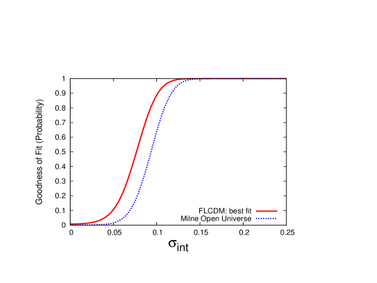
Now let us now calculate the $\chi^{2}$ goodness of fit for two of our cosmological models: a flat best fit $\Lambda$CDM model, and a Milne universe. Let us also assume an additional intrinsic error, $\sigma_{\rm int}$, on top of the error prescribed in the Constitution data set, $\sigma_{i{\rm(data)}}$, so that the total error is $\sigma^{2}_{i}=\sigma_{i{\rm(data)}}^{2}+\sigma_{\rm int}^{2}$. This will allow us to check how sensitive our analysis is to coherent changes in the size of error bars. In Fig. 1 we plot the $\chi^{2}$ goodness of fit for our two theoretical models as a function of $\sigma_{\rm int}$. It can be seen that these two models cannot be easily distinguished from each other using $\chi^{2}$ alone, unless the additional intrinsic error is already known. We also note that the $\chi^{2}$ goodness of fit for the standard flat $\Lambda$CDM model, given the Constitution data without any additional intrinsic errors, is less than $0.6\%$ ($\chi^{2}=465.5$ for $397$ data points).

Figure 1: The $\chi^{2}$ goodness of fit of the Constitution supernova data [7] to a flat $\Lambda$CDM model (red line) and a Milne universe (blue line), assuming additional intrinsic errors added quadratically to the errors specified in the data set. The $\chi^{2}$ goodness of fit for these two models can be seen to be comparable for different values of additional intrinsic error, making them difficult to distinguish without any knowledge of the value of $\sigma_{\rm int}$.

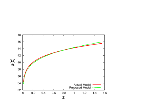
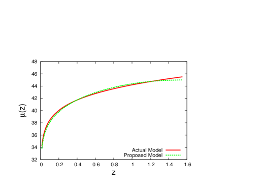
If the real Universe differs from the assumed theoretical model, one would hope that it would be possible to develop a statistical test that would be able to pick up on this. To these ends we consider the ‘crossings’ between the predictions of a given model, and the real Universe from which the data has been derived. Figure 2 shows a schematic picture of what we mean by one crossing (left panel), and two crossings (right panel). In what follows we will use the existence of this type of crossing to develop a new statistic that can be used to determine the goodness of fit between an assumed model and the real Universe.

Figure 2: An idealized schematic plot of one crossing (left panel) and two crossings (right panel) between a proposed theoretical model and the actual model of the Universe when comparing magnitudes as a function of redshift, $\mu(z)$. In reality the actual Universe is observed in the form of data with error bars, of course.

To build our Crossing Statistic in the case of SN Ia data, we must first pick a theoretical or phenomenological model of dark energy (e.g. $\Lambda$CDM) and a data set of SN Ia distance moduli $\mu_{i}(z_{i})$ (e.g. the Constitution data set [7]). As in [12], we use the $\chi^{2}$ statistic to find the best fit form of the assumed model, and from this we then construct the error normalized difference of the data from the best fit distance modulus $\bar{\mu}(z)$:

$$q_{i}(z_{i})=\frac{\mu_{i}(z_{i})-{\bar{\mu}(z_{i})}}{\sigma_{i}(z_{i})}.$$ (2)

Let us now consider the one-point Crossing Statistic, which tests for a model and a data set that cross each other at only one point. We must first try to find this crossing point, which we label by $n_{1}^{\rm CI}$ and $z_{1}^{\rm CI}$. To achieve this we define

$$T(n_{1})=Q_{1}(n_{1})^{2}+Q_{2}(n_{1})^{2},$$ (3)

where $Q_{1}(n_{1})$ and $Q_{2}(n_{1})$ are given by

$$Q_{1}(n_{1}) = \sum_{i=1}^{\rm n_{1}}q_{i}(z_{i})$$

$$Q_{2}(n_{1}) = \sum_{i=n_{1}+1}^{\rm N}q_{i}(z_{i}),$$ (4)

and where $N$ is the total number of data points. If $n_{1}$ is allowed to take any value from $1$ to $N$ (when the data is sorted by redshift) then we can maximize $T(n_{1})$ by varying with respect to $n_{1}^{\rm CI}$. We then write the maximized value of $T(n_{1})$ as $T_{\rm I}$. Finally, we can use Monte Carlo simulations to find how often we should expect to obtain a $T_{\rm I}^{\rm MC}$ larger or equal to the value derived from the observed data, $T_{\rm I}^{\rm data}$. This information can then be used to estimate the probability that the particular data set we have in our possession should be realized from the cosmological model we have been considering.

In our analysis, the process of estimating the distribution of $T_{\rm I}^{\rm MC}$ using Monte Carlo simulations is done in a model independent way as follows. Firstly, a number of different data sets are generated from a single fiducial model, which we take to represent the ‘true’ model of the Universe. The residuals of the fake data are then calculated by subtracting the mean values of the same fiducial model, from which we can then determine $T_{\rm I}^{\rm MC}$. As such, it follows that $T_{\rm I}^{\rm MC}$ does not depend on the background model (which is subtracted away from the generated data to find the residual), but rather on the dispersion about the fiducial model that we haven chosen to adopt. This dispersion is taken to correspond to the errors on the observational data, and so is itself model independent (up to the extent that observers make assumptions about the background cosmology when specifying their value).

Now, before applying the Crossing Statistic to real data, let us first we consider how it fares when applied to simulations. For this we create 1000 realizations of data similar to the Constitution supernova sample based on a fiducial flat $\Lambda$CDM model with $\Omega_{\rm 0m}=0.27$. We then test two different models using the same fake data sets. The first of these is the fiducial model itself (the ‘correct model’), and the second is a flat $\Lambda$CDM model with $\Omega_{\rm 0m}=0.22$ (the ‘incorrect model’). These two models are intentionally chosen to be similar to each other in order to explicitly show the effectiveness of the Crossing Statistic at distinguishing between different models. Next, we add an extra intrinsic dispersion of $\sigma_{\rm int}=0.05$ to the data and test the two models again. This is done to simulate the more realistic situation in which the precise value of $\sigma$ is unknown. Using the simulated data, and applying our statistic, we then test how often the simulated data is sufficient to rule out each of the two models at the $99\%$ confidence level (CL). This data is displayed in Table 1, along with the result of using $\chi^{2}$ alone.

	$\sigma_{\rm int}=0.0$		$\sigma_{\rm int}=0.05$
	$T_{\rm I}$+$\chi^{2}$	$\chi^{2}$	$T_{\rm I}$+$\chi^{2}$	$\chi^{2}$
Correct Model ($\Lambda$CDM with $\Omega_{\rm 0m}=0.27$)	$1\%$	$1\%$	$0.5\%$	$0\%$
Incorrect Model ($\Lambda$CDM with $\Omega_{\rm 0m}=0.22$)	$28.5\%$	$1.9\%$	$26.4\%$	$0\%$

Table 1: A comparison of the $\chi^{2}$ and $T_{\rm I}$ statistics using data simulated from a $\Lambda$CDM model with $\Omega_{\rm 0m}=0.27$. Percentages show the fraction of simulations in which the model in question is ruled out at the $99\%$ confidence level.

It can be seen that with $\sigma_{\rm int}=0$ the $\chi^{2}$ and $T_{\rm I}+\chi^{2}$ statistics both rule out the correct model at $99\%$ CL in $1\%$ of the cases, as should be expected to happen from their definitions. The incorrect model, however, is ruled out by the $\chi^{2}$ statistic at $99\%$ CL in less than $2\%$ of the cases only, while the $T_{\rm I}+\chi^{2}$ statistic is ruled out at $99\%$ CL about $28.5\%$ of the time. This is a significant improvement in distinguishing different models by using a more sophisticated statistic that is extracting more information from the data. Also, when $\sigma_{\rm int}=0.05$ we can see that $\chi^{2}+T_{\rm I}$ is still sensitive to the incorrect model, picking it up and ruling it out at $99\%$ CL in about $26.4\%$ of cases. This is not true of $\chi^{2}$, and clearly demonstrates that $T_{\rm I}$ is much less sensitive to the unknown value of $\sigma_{\rm int}$ than $\chi^{2}$, while being better at distinguishing the correct model from the incorrect one. In fact, even if we over-estimate the size of the error-bars, $T_{\rm I}$ still performs well, and frequently picks out the incorrect model with high confidence.

Figure 3: Residuals with error bars taken from the data (left panel) and the error normalized difference, $q(z)$, (right panel), for a single random realization of supernova data similar to Constitution sample. The simulated data here is based on the fiducial model of flat $\Lambda$CDM with $\Omega_{\rm 0m}=0.27$, and the test model is flat $\Lambda$CDM with $\Omega_{\rm 0m}=0.22$. We assumed here that there is no extra intrinsic dispersion. The crossing point occurs at $z_{1}^{\rm CI}$, and is shown by the vertical blue dashed line. Derived values of $Q_{1}(n_{1}^{\rm CI})$ and $Q_{2}(n_{1}^{\rm CI})$ are also displayed. In the right-hand panel one can see the unbalanced distribution of points around the green zero line (on the right side there are more points below the line, while on the left there are more points above it).

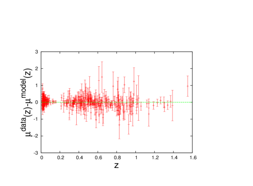
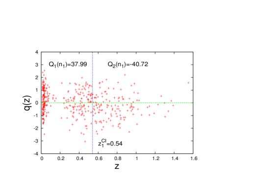
To elaborate further on why $\chi^{2}$ is often not sensitive to using the incorrect model, while $\chi^{2}+T_{\rm I}$ is, let us consider the distribution of residuals with redshift. This is shown in Fig. 3 for a single random realization of data generated from a flat $\Lambda$CDM model with $\Omega_{\rm 0m}=0.27$, and using a test $\Lambda$CDM model that is also flat with $\Omega_{\rm 0m}=0.22$. The distribution of the fake data points is similar to that of the Constitution sample and the data has no extra intrinsic dispersion. The green horizontal dashed line in Fig. 3 is the zero line about which the normalized residuals should fluctuate, when the model being tested and the actual model are the same. The blue dotted vertical line in the right-hand plot represents the redshift at which $T(n_{1})$ is maximized, $z_{1}^{\rm CI}$. The derived values of $Q_{1}(n_{1}^{\rm CI})$ and $Q_{2}(n_{1}^{\rm CI})$ on either side of the blue line are also displayed. For this particular realization of the data the derived $\chi^{2}$ for the test model with $\Omega_{\rm 0m}=0.22$ is $375.72$, which represents a very good $\chi^{2}$ fit to the data considering the number of data points is $557$. The corresponding P-value derived from Monte Carlo simulations is more than $50\%$. However, the derived value of $T_{\rm I}$ is $3102.13$, which comparing with the Monte Carlo realizations results in a P-value of less than $0.5\%$. This shows that the model with $\Omega_{\rm 0m}=0.22$ is strongly ruled out with the $\chi^{2}+T_{\rm I}$ statistic, at the level of $3\sigma$.

Figure 4: The distribution of error normalized difference at different redshifts, as studied in Fig 3. While the overall distribution has a reasonable Gaussian shape, the normalized residuals at $z<0.54$ have a clear shift to the right while those at $z>0.54$ have a clear shift to the left.

This approach can be extended to models with more than one crossing point by the two-point Crossing Statistic. In this case we assume that the model and the data cross each other at two points and, as above, we try to find the two crossing points and their red shifts, which we now label $n_{1}^{\rm CII},z_{1}^{\rm CII}$ and $n_{2}^{\rm CII},z_{2}^{\rm CII}$. This is achieved by defining

$$T(n_{1},n_{2})=Q_{1}(n_{1},n_{2})^{2}+Q_{2}(n_{1},n_{2})^{2}+Q_{3}(n_{1},n_{2})^{2},$$ (5)

where the $Q_{i}(n_{1},n_{2})$ are now given by

$$Q_{1}(n_{1},n_{2}) = \sum_{i=1}^{\rm n_{1}}q_{i}(z_{i})$$

$$Q_{2}(n_{1},n_{2}) = \sum_{i=n_{1}+1}^{\rm n_{2}}q_{i}(z_{i})$$

$$Q_{3}(n_{1},n_{2}) = \sum_{i=n_{2}+1}^{\rm N}q_{i}(z_{i}).$$ (6)

We can then maximise $T(n_{1},n_{2})$ by varying with respect to $n_{1}$ and $n_{2}$, to get $T_{\rm II}$. Comparing $T_{\rm II}$ with the results from Monte Carlo realizations then allows us to determine how often we should expect a two-point crossing statistic that is greater than or equal to the $T_{\rm II}$ obtained from real data. The three-point Crossing Statistic, and higher statistics, can be defined in a similar manner. This can continue up to the N-point Crossing Statistic which is, in fact, identical to $\chi^{2}$. We also note that the zero-point Crossing Statistic, $T_{0}=(\sum_{i}^{\rm N}q_{i})^{2}$, is very similar to the Median Statistic developed by Gott et al. [13]. The Crossing Statistic can therefore be thought of as generalizing both the $\chi^{2}$ and Median Statistics, which it approaches in different limits.

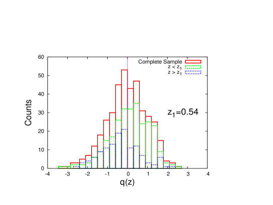
We can also look at the Crossing Statistic from another perspective: In terms of the Gaussianity of a sample about its mean. If an assumed model is indeed the correct one to describe Gaussian distributed data, then the histogram of the normalized residuals should also have a Gaussian distribution, with zero mean and a standard deviation of 1 [15]. To test Gaussianity in this context one can use a variety of different methods, including, for example, the Kolmogorov-Smirnov test [16]. If the histogram instead exhibits significant deviation from the a Gaussian distribution, however, then this can be used to rule out the assumed model. The Crossing Statistic pushes this well known idea from statistical analysis a step further by pointing to the fact that not only should the whole sample of residuals have a Gaussian distribution around the mean, but so should any continuous sub-sample. In our case, these sub-samples should be taken to be those residuals within certain redshift ranges, as discussed above. The importance of our new statement can be realized if we look at Fig. 4 for the $T_{\rm I}$ statistic. While the overall histogram of the normalized residuals may have a Gaussian distribution, this does not mean that the distributions of residuals for the data on either side of the crossing are also Gaussian distributed. It may be the case that the normalized residuals to the left of the crossing point (in redshift range) contribute more to one side of the histogram than the other, and the residuals from the other side of the crossing point do the opposite. In essence, this is what the $T_{\rm I}$ statistic estimates and tests. In the case of $T_{\rm I}$, in fact, we divide the sample up into all possible two sub-samples and we test the Gaussianity for all of them. As can be seen in Fig. 4, while the overall distribution seems to have a reasonable Gaussian shape, the histogram of the normalized residuals at $z<0.54$ has a clear shift to the right, while those at $z>0.54$ are shifted to the left. In our analysis, deviation from Gaussianity with zero mean is calculated by derivation of $Q_{1}(z_{1})$ and $Q_{2}(z_{1})$ which are, in fact, the areas under the histograms on the two sides of the zero mean. This is a simple, but robust way, to test the hypothesis above.

3 Results

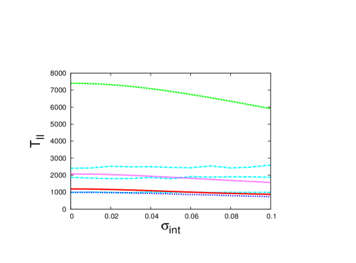
Now let us apply our Crossing Statistics to a suite of different models. We will calculate $\chi^{2}$, $T_{\rm I}$, $T_{\rm II}$ and $T_{\rm III}$ for (i) the best fit flat $\Lambda$CDM model (with $\Omega_{\rm 0m}=0.288$ when $\sigma_{\rm int}=0$), (ii) a best fit asymptotically flat void model with $\Omega_{\rm 0m}=0.28$ at the centre, and with FWHM at $z=0.66$ when $\sigma_{\rm int}=0$, (iii) a flat $\Lambda$CDM model with $\Omega_{\rm 0m}=0.22$, and (iv) the Milne open universe. We use the Constitution data set [7], and vary the additional intrinsic error, $\sigma_{\rm int}$, between $0$ and $0.1$ magnitudes. In Fig. 5 we compare these statistics with the confidence limits that result from $1000$ Monte Carlo realizations of the error bars, for each value of $\sigma_{\rm int}$. This is done in a completely model independent manner.

Figure 5: The $\chi^{2}$, $T_{\rm I}$, $T_{\rm II}$ and $T_{\rm III}$ statistics for a best fit flat $\Lambda$CDM model (red lines), a void model (blue dashed lines), the Milne universe (green dashed lines) and a flat $\Lambda$CDM model with $\Omega_{\rm 0m}=0.22$ (pink dotted lines). The analyses are performed using the Constitution supernova data [7], and by assuming various different additional intrinsic errors. The confidence limits from $1000$ Monte Carlo realizations of the error-bars are derived in a completely model independent manner. It can be seen the $\chi^{2}$ statistic fails to distinguish between these models with any degree of significance, and that by assuming additional intrinsic errors this statistic allows all models to be made consistent with the data. The $T_{\rm I}$ crossing statistic, on the other hand, rules out the Milne universe to more than $5\sigma$, and also the flat $\Lambda$CDM model with $\Omega_{\rm 0m}=0.22$ to nearly $3\sigma$, even when the amount of additional intrinsic error is large.

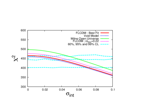
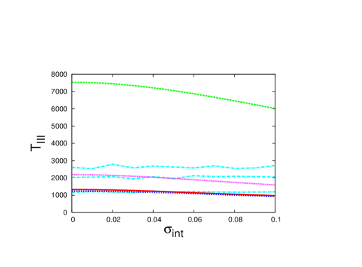
It can be seen from Fig. 5 that the $\chi^{2}$ statistic (upper panel) cannot easily be used to distinguish between the different models with a high degree of confidence, especially if we do not know $\sigma_{\rm int}$. Indeed, if we add $\sigma_{\rm int}=0.1$ magnitudes to the data then all four models become a good fit, at the $60\%$ confidence level. Alternatively, with $\sigma^{2}_{\rm int}=0$ all four models are outside of the $99\%$ confidence level. This illustrates the ineffectiveness of $\chi^{2}$ as a statistic for determining the goodness of fit when the errors on the data are not well known.

The results for the one-point Crossing Statistic are shown in the second panel from the top in Fig. 5. In terms of this statistic it can be seen that the best fit flat $\Lambda$CDM model and the best fit void model are now very much consistent with the data, even with no additional intrinsic error. At the same time, it is also clear that the Milne universe lie well outside the $99\%$ confidence level and the flat $\Lambda$CDM model with $\Omega_{\rm 0m}=0.22$ lie well outside the $95\%$ confidence level, even when $\sigma_{\rm int}$ is large. In the third and fourth panels in Fig. 5 we see the results for the two-point and three-point Crossing Statistics, respectively. The Milne Universe remains outside the $99\%$ confidence level in each of these, for the range of $\sigma_{\rm int}$ considered, while the flat $\Lambda$CDM model with $\Omega_{\rm 0m}=0.22$ now lies mostly within the $60$-$99\%$ confidence region.

This difference in probability of the different Crossing Statistics for the $\Lambda$CDM model with $\Omega_{\rm 0m}=0.22$ is due to this model having only one ‘crossing’ with the data. Adding extra hypothetical crossings then has little affect on $T_{i}$, as the extra crossing points all cluster around the same $z$. A model that fits the data better, with many crossings, however, should be expected to have $T_{i}$ statistics that increase with $i$. On this basis, one can then argue that for a model to be considered consistent with the data it must show consistency across all crossing modes. The point here is that if there is a significant crossing of the data and the model, then it should show up in the Crossing Statistics as a failure of $T_{i}$ to decrease sufficiently with decreasing $i$. A flat $\Lambda$CDM model with $\Omega_{\rm 0m}=0.22$ is therefore considered non-viable at close to $3\sigma$ because of the discrepancy in $T_{\rm I}$, even though $T_{\rm II}$ and $T_{\rm III}$ show some degree of consistency.

One should notice that $\Delta\chi^{2}$ with respect to the best fitting point in the parameter space can be used in deriving the confidence only in cases where we know the correct underlying theoretical model. If we assume an incorrect theoretical model there will still be a best fit $\chi^{2}$ point in the parameter space, and we can still define $1\sigma$, $2\sigma$ or $n\sigma$ confidence limits, but this then has little or nothing to do with goodness of fit or whether the assumed model is correct or not. While we do not know the size of the error bars, playing with the $\sigma_{\rm int}$ can also help an incorrect model to achieve a $\chi_{\rm red}^{2}$ of one (or close to one) for the best fitting point in its parameter space. On the other hand, while defining the confidence limits depends on $\Delta\chi^{2}$ and the degrees of freedom in the assumed parametric model, the $\Delta\chi^{2}$ between two models (or even two points in the parameter space of one model) changes with changing $\sigma_{\rm int}$ while the degrees of freedom of the assumed models are fixed.

4 Conclusion

In summary, we have presented a new statistic that can be used to distinguish between different cosmological models using their goodness of fit with the supernova data. Previous work on this subject has analyzed the residuals from supernova data, and in particular has examined pulls [18]. In these analyses, however, the correlations as functions of redshift have not been examined. Here we have included this extra information, and have shown that the different Crossing Statistics that have been derived as a result are sensitive to the shapes and trends of the data and the assumed theoretical model. These statistics are in general also less sensitive to the unknown intrinsic dispersion of the data than $\chi^{2}$, as exemplified by the fact that the consistency between a model and a data set does not change much even when we assume large additional intrinsic errors. The Crossing Statistic can be used in the process of parameter estimation, and for this purpose it can be put in the category of shrinkage estimators [19] (as raw estimates are improved by combining them with other information in the data set). The $\chi^{2}$ method, as an example of a maximum likelihood estimator, is a very good summarizer of the data, but does not extract all of the available statistical information. We have shown here that by using $T_{\rm I}$, $T_{\rm II}$ etc. we can extract more information from the data, and use this to make more precise statements about the likelihood of different parameters and models.

Let us now mention some of the important remaining issues that need to be resolved in the context of the Crossing Statistic. So far, in all our analyses, we have considered uncorrelated data. The Constitution supernova data set [7] that we have used in our analysis is, in fact, strictly uncorrelated (as all off-diagonal elements of the correlation matrix are zero). However, in reality this will only be approximately true, and the most recent methods of supernova light-curve fitting results in data sets with slight correlations between the individual data points [21]. It is an important question as to how best to modify the Crossing Statistic to take account of such correlations, as this would broaden the application of the Crossing Statistic to a much wider category of problems. Another important issue involves comparing the Crossing Statistic with Bayesian methods of model selection. The Crossing Statistic proposed in this paper is by nature a frequentist approach, and is able to deal with different models without any prior information. In contrast, Bayesian methods require priors that play an important role in model selection and parameter estimation. This will complicate comparisons, which will depend on whether we are dealing with completely unknown phenomena (for which we have no prior information), or with phenomena where we have some prior information available. These issues will be the subject of future work, and their results will reported elsewhere.

Finally, let us briefly mention the “Three Region Test” proposed by [20] that detects and maximizes the deviation between the data and a hypothesis in three bins. This test uses normalized residuals to test the goodness of fit in a similar way to our Crossing Statistic, but is considerably less general.

The Crossing Statistic appears to us to be a promising method of confronting cosmological models with supernovae observations, and has the potential to be straightforwardly generalized to other datasets where similar problems occur.