Simulating Redshift-Space Distortions for Galaxy Pairs with Wide Angular Separation
Abstract
The analysis of Redshift-Space Distortions (RSD) within galaxy surveys provides constraints on the amplitude of peculiar velocities induced by structure growth, thereby allowing tests of General Relativity on extremely large scales. The next generation of galaxy redshift surveys, such as the Baryon Oscillation Spectroscopic Survey (BOSS), and the Euclid experiment will survey galaxies out to , over –. In such surveys, galaxy pairs with large comoving separation will preferentially have a wide angular separation. In standard plane-parallel theory the displacements of galaxy positions due to RSD are assumed to be parallel for all galaxies, but this assumption will break down for wide-angle pairs. Szapudi (2004) and Papai & Szapudi (2008) provided a methodology, based on tripolar spherical harmonics expansion, for computing the redshift-space correlation function for all angular galaxy pair separations. In this paper we introduce a new procedure for analysing wide-angle effects in numerical simulations. We are able to separate, demonstrate, and fit each of the effects described by the wide-angle RSD theory. Our analysis highlights some of the nuances of dealing with wide-angle pairs, and shows that the effects are not negligible even for relatively small angles. This analysis will help to ensure the full exploitation of future surveys for RSD measurements, which are currently confined to pair separations less than out to .
keywords:
cosmological parameters — large scale structure of Universe — cosmology : observations — methods : analytical1 Introduction
Many different mechanisms have been suggested to explain the observed late-time acceleration of the expansion of the Universe (Riess et al., 1998; Perlmutter et al., 1999).111For a recent review of dark energy see, e.g., (Frieman, Turner & Huterer, 2008) and references therein. Differentiating between these options is one of the main challenges facing cosmologists today. We can try to build up the evidence for different mechanisms by examining the evolution of the Universe in two key ways: measuring the background geometry and measuring structure formation within it.
The geometrical evolution of the Universe can most easily be measured using two primary techniques: we can use supernovae as standard candles or galaxy clustering as a standard ruler to make precise measurement of cosmological expansion. Although supernovae were first to confirm the accelerated expansion of the Universe at high statistical significance (Riess et al., 1998; Perlmutter et al., 1999) following analyses of early galaxy surveys (Efstathiou et al., 1990), supernovae surveys are now limited by systematic rather than statistical errors (Kessler, 2009). The possibility of using galaxy clustering to provide a standard ruler has become increasingly important since the baryon acoustic peak was detected (Percival et al., 2001; Cole et al., 2005; Eisenstein et al., 2005) in galaxy power spectra measured from the 2dF Galaxy Redshift Survey (2dFGRS; Colless et al. 2003) and the Sloan Digital Sky Survey (SDSS; York et al. 2000). Using only the Baryon Acoustic Oscillation (BAO) component of the galaxy clustering signal makes constraints robust to non-linear effects, and has already been exploited to produce interesting constraints on cosmological models (Percival et al., 2007a, b; Gaztanaga et al., 2008; Sanchez et al., 2009; Percival et al., 2010).
Galaxy surveys provide complementary information about the build-up of large-scale structure through Redshift Space Distortions (RSD). These arise because we do not observe true galaxy positions, but instead infer distances from measured redshifts. Coherent comoving galaxy velocities due to the growth of structure therefore lead to measurable anisotropic clustering (Kaiser, 1987; Hamilton, 1998). RSD have been measured from the 2dFGRS and SDSS using techniques based on both correlation functions and power-spectra (Peacock et al., 2001; Hawkins et al., 2003; Percival et al., 2004; Pope et al., 2004; Zehavi et al., 2005; Okumura et al., 2008; Cabre & Gaztanaga, 2009), and have recently been detected at higher redshift (Guzzo et al., 2009; Blake et al., 2010).
In fact, for fundamental reasons, RSD are independent of galaxy bias: galaxies act as test particles in the matter flow, so their motion is independent of galaxy properties. We can therefore measure the matter velocity field at the locations of the galaxies and, provided that galaxy positions are representative within the velocity field, this gives an unbiased measurement of where , the logarithmic derivative of the linear growth rate, , with respect to the scale factor , and quantifies the amplitude of fluctuations in the matter density field.
Many techniques have been proposed for measuring RSD, including using multipoles of the correlation function (Hamilton, 1992), or the power spectrum (Percival & White, 2009), based on the plane-parallel approximation for RSD (Kaiser, 1987). The geometry of the system can be easily incorporated into an analysis of the correlation function as the separation of each pair can be split into radial and angular components. It is more difficult to perform such a decomposition when measuring the power spectrum, although various techniques have been suggested, decomposing the density field into a basis of spherical harmonics and radial functions (e.g. Fisher et al. 1994; Heavens & Taylor 1995). As well as allowing for the geometry to a survey and RSD within it, we need to allow for two effects:
- 1.
-
2.
as noted by Hamilton (1998), the full RSD operator has extra terms compared to the plane-parallel one and results in a redshift-space power spectrum which is not diagonal in . These extra terms are important for galaxy pairs separated by wide angles and need to be included in any analysis that uses wide-angle data (Szalay et al., 1998; Szapudi, 2004; Papai & Szapudi, 2008).
In this paper we concentrate on the second of these effects. Szapudi (2004) and Papai & Szapudi (2008) proposed a method of computing the redshift-space correlation function which does not assume a plane-parallel approximation and is applicable to arbitrarily large angles. In their treatment the redshift-space correlation function depends not only on the redshift-space pair separation and cosine of the angle of the pair with respect to the line-of-sight , but also on the separation angle between two galaxies in a pair , which does not have to be small. They were able to express the redshift-space correlation function explicitly trough a real-space correlation function and cosmological parameters. Given the precision that future surveys will achieve and the fact that they will cover large fractions of the sky, these effects will need to be corrected.
The wide-angle effects can be subdivided in “purely wide-angle” and “mode-coupling” terms: “purely wide-angle” effects correct plane-parallel predictions accounting for the fact that the separation angle is non-zero, “mode-coupling” terms in addition account for the fact that galaxy pairs coherently moved from the high-density to low-density regions. These latter terms vanish if the initial real-space distribution of galaxies is uniform in distance, and both terms vanish in the plane-parallel limit due to the symmetry of the system. Both terms are of the same order and mode-coupling tends to smooth out features in the power spectrum such as the Baryon Acoustic Oscillations (BAO).
Given the importance and, particularly, the quality of RSD constraints expected from forthcoming surveys such as the Baryon Oscillation Spectroscopic Survey (BOSS; Schlegel et al. 2009a), surveys resulting from proposals for wide-field multi-object spectrographs on 4m telescopes such as BigBOSS (Schlegel et al., 2009b) and satellite missions such as Euclid (Laureijs et al., 2009), it is timely to revisit this problem, and to test wide-angle RSD theory. In this paper we use numerical simulations to extensively test the dependence of RSD constraints on the angular separation of galaxy pairs.
This paper is organised as follows: in Sec. 2 we briefly review the theory of wide-angle RSD; in Sec. 3 we describe a time-efficient method of getting a low-noise measurement of wide-angle correlation function from a mock HV catalog; in Sec. 4 we present our results and discuss all the steps necessary to match measured correlation function with theoretical predictions; in Sec. 5 we conclude and discuss how the results will affect real survey measurements.
2 Wide-Angle Redshift-Space Distortions
Galaxy positions are measured in a redshift-space, and differ from the real-space positions because of the contributions from peculiar velocities,
| (1) |
where is the redshift space position, is the real space position and the radial component of peculiar velocity.
Since the total number of galaxies in real and redshift spaces is the same, the number of galaxies observed in a volume element of redshift space is related to the real space number density by:
| (2) |
The observed redshift space galaxy overdensity at position can be related to the redshift-space selection function ,
| (3) |
In contrast, an unbiased estimate of the true galaxy overdensity at position is given by:
| (4) |
where is the expected galaxy distribution in real-space – the expected number density of unclustered galaxies at position given the selection criteria of the survey.
We distinguish here between the measured redshift-space selection function and the true selection function even though the two are the same at linear order. We now assume that the expected density is a function of the radial component of the position only, which we denote in redshift-space and in real-space. Thus the relation between the observed redshift space overdensity and the true overdensity is:
| (5) |
Using Eq. (2) we obtain:
| (6) | ||||
which gives, to linear order:
| (7) |
where
| (8) |
Usually the term in the Jacobian is omitted because, in the linear regime, it gives rise to a term, that would tend to zero at large distances. However, Papai & Szapudi (2008) have argued that, for wide angles, the term is of the same order as the term.
Using the exact Jacobian, and following Papai & Szapudi (2008), we can express the linear overdensity as:
| (9) |
so the correlation function is:
| (10) |
where are the Legendre polynomials of order and is the real-space matter power spectrum. The third terms in the brackets are the ones responsible for the wide-angle effects, while the fourth terms are the ones responsible for the mode-coupling. Note that the and terms in the denominator depend on the angular separation of the galaxies. Setting as the angle between the vector to the first galaxy in a pair , to be the vector connecting galaxies in a pair, and to be the angle between vector to the second galaxy in a pair and , we can use the sine rule (see Fig. 1) to express and as
| (11) | |||
| (12) |
Tripolar spherical harmonics are the most natural basis for the expansion of a function that depends on three directions (Varshalovich et al., 1988) so, as suggested in Szapudi (2004) and Papai & Szapudi (2008), we expand Eq. (10) using a subset of them that are proportional to the zero angular momentum:
| (13) | |||
where are normalized spherical functions, multiplied by the Wigner symbol. The redshift space correlation function is then written as:
| (15) |
where are a series of coefficients that depend on , and , and they can be divided into wide-angle components (given in Szalay et al. 1998 & Szapudi 2004) that do not depend on the third term in Eq. (9), and mode-coupling components (given in Papai & Szapudi 2008); the plane-parallel approximation emerges as a limit when .
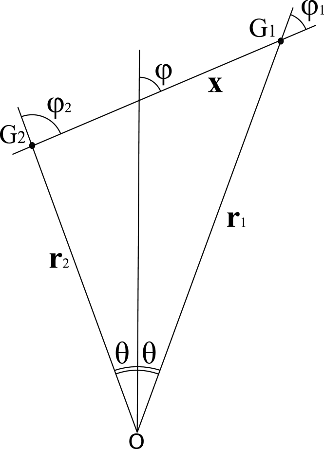
As described in Hamilton & Culhane (1996), for any pair of galaxies we can fully analyse the problem within a plane formed by the two galaxies and the observer; the effect of redshift-space distortions only depends on the geometry within this plane. In the coordinate system described above, the vectors connecting the observer with the galaxies are and , and the separation vector between the galaxies is ; are the angles between and . In the plane parallel approximation . This description of the triangle is shown in Fig. 1.
At this point we still have the freedom to choose a line-of-sight to the galaxy pair: we follow the standard approach and choose the line of sight as a direction bisecting the angle formed by the two galaxies, which we assume is given by . The angle between the angle bisector and is denoted , and we define . We therefore have that , and . This is shown in Fig. 1.
3 Measuring Wide-Angle Correlation Functions
A standard method for analysing a N-body simulation to test wide-angle redshift-space distortions would be to:
-
1.
locate an observer within the output,
-
2.
translate all galaxies from real into redshift-space based on this observer,
-
3.
sample from these galaxies based on desired radial distribution,
-
4.
split pairs into bins in , , and counts pairs,
-
5.
estimate the correlation function.
This approach mimics that of an actual survey analysis, creating a mock galaxy catalogue. However, if we want to measure the effect of redshift-space distortions for galaxy pairs with a particular angular separation, the method is not optimal as only a small fraction of the galaxy pairs analysed will have this angular separation. In addition, we have to perform the full procedure for every radial galaxy distribution that we wish to analyse, and this distribution will limit the pair-density that can be selected from the simulation. In order to rapidly increase the signal-to-noise, we adopt a different procedure, allowing the origin to move so that each galaxy pair can be analysed as if it was observed with the required angular separation. This procedure can be summarised as follows:
-
1.
decide on the value of for which we wish to analyse pairs,
-
2.
take each galaxy pair from the simulation with real-space separation ,
-
3.
for each pair randomly choose ,
-
4.
choose the location of the origin giving this and ,
-
5.
move galaxies according to their expected redshift-space distortion,
-
6.
weight the pair by a function of to match desired distribution,
-
7.
split pairs into bins in , and counts pairs,
-
8.
estimate the correlation function.
The added complexity of including redshift-space distortions on a pair-by-pair basis is outweighed by the ability to obtain more pairs at the desired angular separation. Note that in step (iii) is constrained and cannot have any value within because results in geometrically impossible triangles (see, Fig. 1). The distributions of triangles in and for a galaxy distribution with a power law selection in can be calculated analytically, as we now demonstrate.
3.1 Real-space distribution of ,
The redshift-space correlation function in Eq. (17) depends on the selection function , where is the number density of galaxies in real space and is the position of the galaxy from the observer as in Section 2. If the galaxy distribution is uniform (, , both independent of ), then the probability of finding a galaxy in some region is proportional to the volume of that region. Therefore if we randomly pick a galaxy in the catalog, there will be on average galaxies in a small volume element which is distance away from that galaxy within an angular slice . In the plane-parallel approximation, where all galaxies are assumed to lie along the same direction from the observer, the distribution of galaxy pairs will scale as
| (18) |
where is the number of pairs with separation and cosine of the angle with the line of sight in the interval. If we pick galaxy pairs separated by a fixed opening angle from the uniform spatial distribution of galaxies (step (i) in the procedure described above), for a large enough angle the distribution of pairs will not follow Eq. (18). For galaxy pairs with a fixed half-angle (see, Fig. 1), the likelihood of finding one galaxy at position and another at is , . Since the two likelihoods are independent, the joint probability of finding that pair of galaxies is:
| (19) |
Using Eqs. (11) and (12) we can rewrite Eq. (19) in terms of and as:
| (20) |
After completing steps (ii) and (iii) in the previous subsection, we will have a distribution of galaxy pairs that is uniform in and scales as with separation. This distribution of galaxy pairs does not correspond to . If we want to compare our data with the correlation function computed from Eq. (17) for , we have to weight our galaxy pairs (step (iv) in the previous subsection) by an additional factor of to get a distribution given by Eq. (20).
This procedure can be applied to the case of arbitrary . If, for example, the galaxy number density scales as a power-law , then , and the distribution of galaxy pairs with a fixed opening half-angle drawn from this distribution will be:
| (21) |
We therefore weight all pairs recovered from the simulation with a weight given by:
| (22) |
where is the separation of the galaxies in redshift-space, is the real-space value of for the chosen galaxy pair and is the redshift-space value. We divide the real-space distribution by the redshift-space equivalent in order to normalise the weights to give no net change in the expected pair distribution.
3.2 Redshift-space distribution of ,
When transformed into redshift space, the real-space galaxy distribution is “washed out” by the random component of galaxy velocities, so we need to convolve with the random velocity distribution. This would normally not be a problem as we would estimate the galaxy distribution directly in redshift-space. However, using the above procedure we have set the real-space distribution of galaxies, so we need to take care when modelling the redshift-space distribution. To correct for this effect, we first estimate the velocity dispersion from the catalog, assuming that the random velocities are drawn from a Gaussian distribution. We then convolve the initial distribution in real space with this Gaussian. For example, for , the probability of finding a galaxy at distance away from the observer is . In the unclustered redshift space this will transform into:
| (23) | |||||
where F is a hypergeometric function.
For a specific case of , Eq. (23) results in:
| (24) |
where is an error function. The distribution of galaxy pairs for will be:
| (25) |
where is given by Eq. (24) and and can be expressed in terms of and via Eqs. (11) and (12), after the substitution of with .
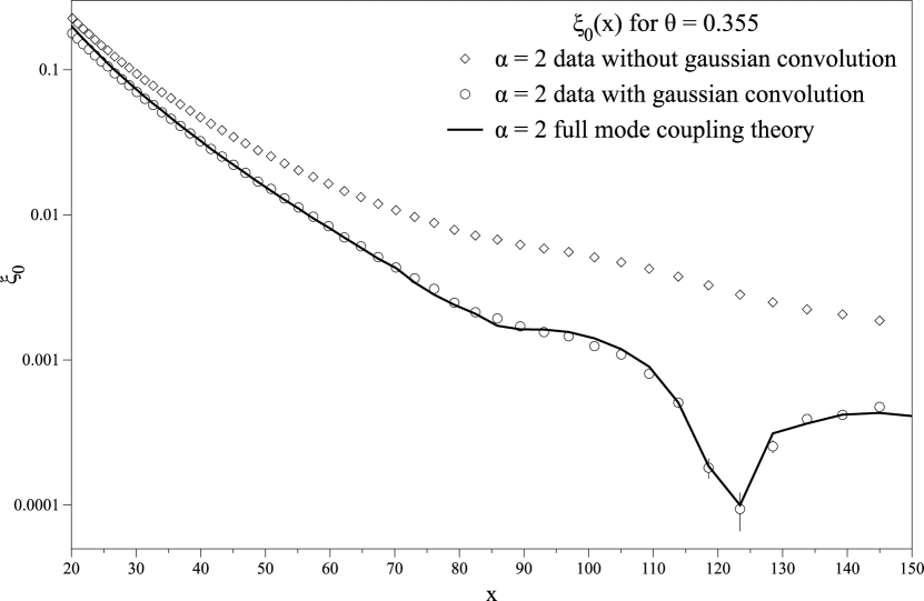
When modelling the theoretical correlation function, Hamilton & Culhane (1996) argue that the difference between and is small. While this is true when creating a model correlation function, it is not true, and we need to use the instead of , when we model the data. This is shown in Fig. 2, where we plot calculated for from a mock catalog, assuming that the galaxy distribution follows the one expected from either the real-space or redshift-space calculation. See Section 4 for more details of the calculation.
3.3 Pairs close to the origin
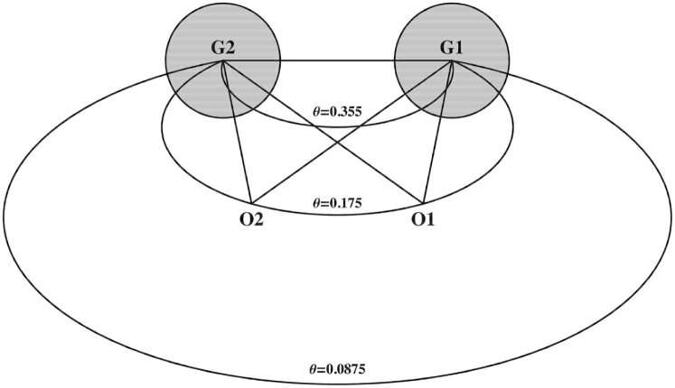
Galaxies that are close to the origin can cause problems as, for such galaxies, the redshift-space displacement can be larger than the distance to the galaxy. This problem is exacerbated because we do not include the velocity of the observer in our calculation. In extreme situations, naively applying the expected redshift-space distortion would place the galaxy on the opposite side of an observer. In order to avoid such problems, we only include galaxy pairs where both galaxies are more than away from the origin, where is the 1D velocity dispersion of the galaxy population. For the HV simulation . Fig. 3 shows, for galaxies and , the loci of positions at which the origin could be placed for fixed . The circles mark the exclusion zones. If one of the galaxies in a pair is inside the exclusion zone in real space, we do not include that pair when we estimate the correlation function. This exclusion is tracked when we calculate the expected galaxy distribution.
3.4 The Hubble Volume Simulation
We apply the procedure outlined in Sec. 3 to analyse wide-angle redshift-space distortions within the CDM Hubble Volume (HV) simulation (Evrard et al., 2002). The CDM HV simulation, covering a box, assumes a cosmological model with , , , , , , & . We do not apply any galaxy bias, simply Poisson sampling the matter particles to give our “galaxy distribution”; the inclusion of a bias model would not alter the conclusions of this work. We use the periodic nature of the numerical simulation to eliminate boundaries from our pair counts. This means that, by using the above weighting scheme and allowing for the removal of galaxies close to the origin, the expected number of galaxy pairs in the absence of clustering can be calculated analytically. We can therefore use the natural estimator (Landy & Szalay, 1993), where is the measured number of galaxy-galaxy pairs.
4 Results
We have performed 100 runs, each based on a sample of galaxies drawn from the output of the HV CDM simulation. For each unique pair of galaxies within the sample we have selected two locations for the origin, one where the galaxies subject a separation angle of , chosen to match figure 1 of Papai & Szapudi (2008), and one origin where , twice this angular separation, to emphasise the wide angle effects on pairs separated by a very wide angle.
We include all pairs with redshift-space separation , and each pair was weighted as described in Section 3.2, based on its real-space separation and angle to the line of sight. Given that, as one can see from Eq. (10), the mode-coupling terms depend strongly on the radial galaxy distribution, for both the aperture angles we selected samples with different radial galaxy distributions, in order to test our methodology in different cases; we chose :
-
•
corresponds to the case of a galaxy distribution that has equal density in radial bins of equal width. In this case there are no mode-coupling terms in Eq. (10), so this corresponds to the ”pure wide angles” case.
-
•
corresponds to a final real-space distribution of galaxy pair separations with probability density function proportional to . This is the same distribution obtained by randomly sampling pairs from the simulation, so the factor drops out of Eq. (22). Note that, for clarity, we do not present results from this value of as they are very similar to, and overlap results for . The match between data and theory has the same quality as for the other values of .
-
•
matches a distribution of galaxies that are uniformly distributed in volume, so equal volumes contain equal numbers of galaxies. Most planned surveys aim to observe galaxies with this radial distribution. Note that, for this galaxy distribution, the pair distribution goes as .
-
•
represents a steeper radial distribution where more galaxies are found at larger distances. This will increase the effect of the mode-coupling terms in the wide-angle redshift-space distortion formulae (Eq. 22).
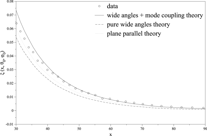
We have calculated errors by comparing outputs from 100 subsamples, that cover the same HV volume and so only contain the shot noise element. These errors will therefore underestimate the true error, because they do not fully include the cosmic variance component. However, the HV volume is , and we only consider pairs with , so we expect the shot noise to dominate the error budget. Even so, it is worth pointing out that our primary aim is to consider deviations from plane-parallel theory and that our proposed methodology works to match data with the full mode-coupling theory: the size of the errors is unimportant, provided they are far smaller than the differences between theories.
Fig. 4 shows the correlation function, calculated within a narrow bin in for and ; this is equivalent to figure 1 of Papai & Szapudi (2008). We are able to fit the theoretical correlation function to the estimate from HV simulations for scales larger then (we do not expect to match perfectly data with theory on smaller scales because we didn’t model non-linearities). Looking at plane-parallel, pure wide-angle and full mode-coupling theories, it is clear that only the full mode-coupling theory provides a good fit to the data.

Fig. 5 shows the ratio between the correlation function predicted by the full mode-coupling theory and that for the plane-parallel case, as a function of , for a fixed value of , with ; from this plot we can see that even for small angles there is a non negligible difference.
In order to analyse RSD, the measured correlation function is usually decomposed into Legendre momenta, which contain all of the RSD signal (Hamilton, 1998). Some combination of these momenta is then used to constrain cosmological parameters through their effects on the growth of structure. To see how wide angle effects would modify these measurements we estimate first three even Legendre momenta of the correlation function from HV mock catalog. We measure:
| (26) |
for . Adopting the plane-parallel philosophy (Hamilton, 1992), one might be tempted to interpret these functions as:
| (27) | |||||
| (28) | |||||
| (29) |
where is a real space correlation function and . In fact the functions in Eq. (26) are given by:
| (30) |
where is a weight function that appears because of geometrical constraints and because the distribution of will not be uniform. We do not correct for this weight in our measurement from simulations, and apply it to the theoretical calculations that we compare against.
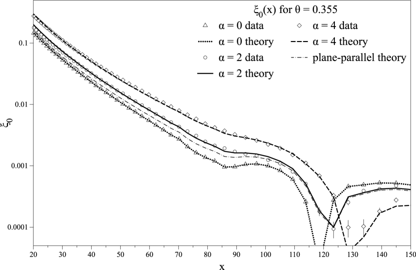
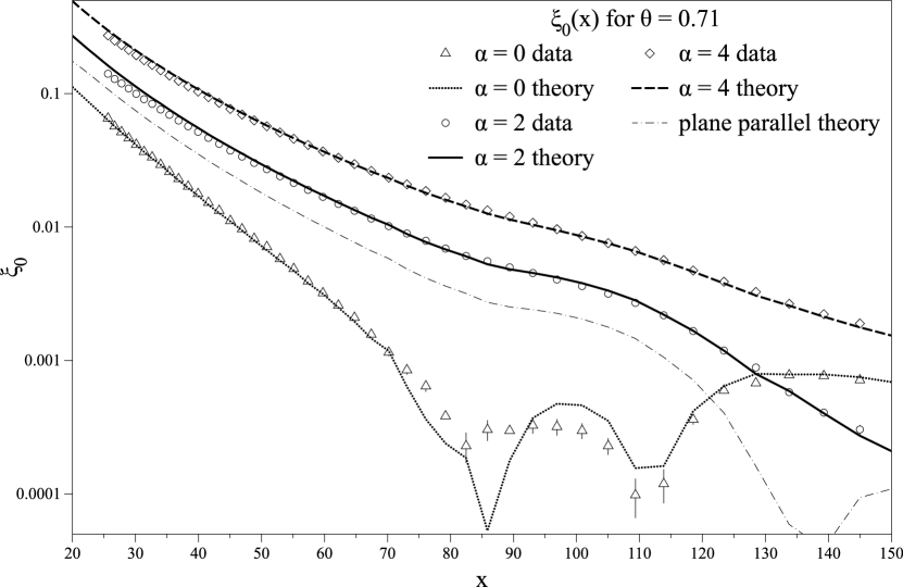
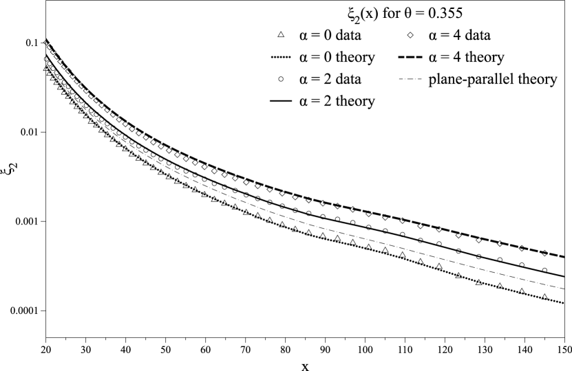
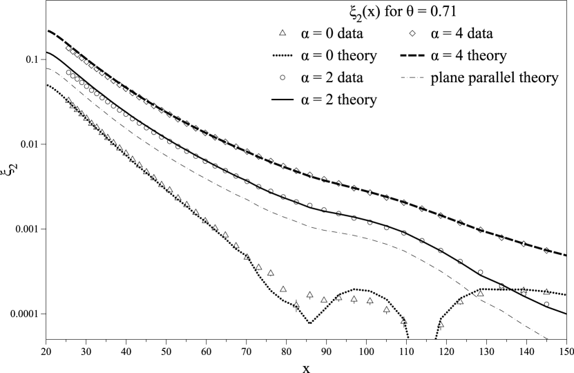
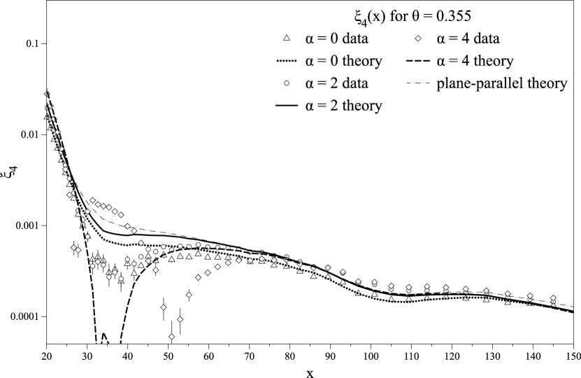
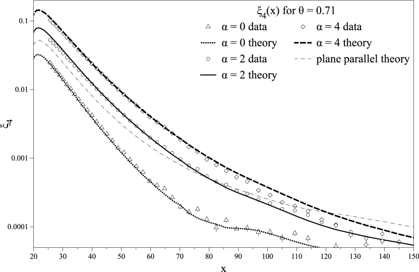
Fig. 6 presents the main results of this work, showing the application of our methodology to sample and analyse data, and comparing against the full mode-coupling predictions. We plot , , for both the aperture angles and for radial galaxy density distributions corresponding to , and ; as we can see, the contribution of the mode coupling terms increase with , and as the radial galaxy distribution steepens, more galaxies are moved nearer by the RSD, leading to an increase in the small-scale correlation function. Momenta of the correlation function computed with the full mode coupling theory match remarkably well the data analysed as explained in Sec. 3. We also plot the plane-parallel prediction as a comparison, and this demonstrate how badly this approximation fails for galaxy pairs with wide angular separation. The only parts where our methodology do not match the mode coupling theory are where the correlation multipoles are very small (around ) or for small scales, where non-linearities become important; we also have to take in account that, for the steeper galaxy distributions, we are upweighting results from the same number of pairs as the more shallow galaxy distributions so, although the signal is stronger, the relative error will be the same.
5 Discussion and conclusions
Redshift-Space Distortion Analyses are a powerful tool for cosmology, but incoming data need to be analysed very carefully in order to fully extract all available information. Until now RSD analyses have concentrated on using the plane-parallel approximation (with a few exceptions including Okumura et al. 2008; Pope et al. 2004; Matsubara 2004); this is almost correct if the survey is narrow, but when galaxy surveys with wide field of view data will be available, there will be a consistent number of galaxy pairs separated by wide angles and in this case the plane-parallel approximation fails.
This approximation arises from not taking in account some of the terms in the Jacobian relating redshift- to real-space; in this paper we considered its exact expression, and this causes additional, non-diagonal terms in the correlation function. We then use the expansion of the correlation function in a base of tripolar spherical harmonics, as suggested in Papai & Szapudi 2008; following the formalism developed in Szapudi 2004; Papai & Szapudi 2008, we make predictions for the momenta of the correlation function for galaxy pairs at fixed angular separation, and we test them against data from the Hubble Volume Simulation.
In order to do this we have had to introduce a new methodology: rather than creating a single sample of galaxies in redshift-space from which we can count pairs, we have instead dynamically applied RSD on a pair-by-pair basis, choosing an origin for each. By including weighting functions in and we can match results from the more traditional approach. This allows us to only consider galaxy pairs at particular values of .
To show both the correctness of our methodology and the deviation from the plane-parallel situation we tested galaxies separated by two different fixed values of ; the mode coupling terms are also strongly dependent on the galaxy radial distribution, so we have tested simulations with 4 different number density distributions, for both values of .
We show that taking in account the wide angle and mode coupling terms (that are of the same order, as stated in Papai & Szapudi 2008) give a clear deviation from the plane-parallel theory; using the exact theory and our methodology, we can match the results of simulations, the agreement between data and theory being remarkable, especially considering how crude our modelling of the HV simulations is (we use a measurement of the 3D real-space correlation function as our baseline model, and we do not include a correction for fingers-of-god type effects). For RSD measurements made within radial bins, it will be vital to match the theory to the exact distribution of galaxies observed.
In a measurement of RSD from real data, the final result will be a weighted average over different opening angles, to take account for the fraction of galaxy pairs separated by a angle, so in wide surveys one has to discard the plane-parallel approximation, or face losing a considerable amount of information. For this reason our methodology will be particularly useful for incoming and future redshift Surveys, such as the Baryon Oscillation Spectroscopic Survey (BOSS; Schlegel et al. 2009a), BigBOSS (Schlegel et al., 2009b), and Euclid (Laureijs et al., 2009); the importance of this methodology for current and future experiments will be considered in a subsequent paper (Samushia et al., in preparation).
6 Acknowledgements
AR is grateful for the support from a UK Science and Technology Facilities Research Council (STFC) PhD studentship. WJP is grateful for support from the European Research Council and from the Leverhulme Trust and STFC. LS acknowledges support from European Research Council, Georgian National Science Foundation grant ST08/4-442 and SNSF (SCOPES grant No 128040). AR would like to thank G. W. Pettinari for the useful discussions. Simulated data was calculated and analysed using the COSMOS Altix 3700 supercomputer, a UK-CCC facility supported by HEFCE and STFC in cooperation with CGI/Intel.
References
- Ballinger et al. (1996) Ballinger W. E., Peacock J. E., Heavens A. F., 1996, MNRAS, 282, 877
- Blake et al. (2010) Blake C., et al., 2010, MNRAS accepted, [arXiv:1003.5721]
- Cabre & Gaztanaga (2009) Cabre A., Gaztanaga E., 2009, MNRAS, 396, 1119
- Cole et al. (2005) Cole S., et al., 2005, MNRAS, 362, 505
- Colless et al. (2003) Colless M., et al., 2003, astro-ph/0306581
- Eisenstein et al. (2005) Eisenstein D.J., et al., 2005, ApJ, 633, 560
- Evrard et al. (2002) Evrard A.E., et al., 2002 ApJ, 573, 7
- Efstathiou et al. (1990) Efstathiou G., Sutherland W.J., Maddox S.J., 1990, Nature, 348, 705
- Fisher et al. (1994) Fisher K.B., Scharf C.A., Lahav O., 1994, MNRAS, 266, 219
- Frieman, Turner & Huterer (2008) Frieman J., Turner M., Huterer D., 2008, Ann. Rev. Astron. Astrophys., 46, 385
- Gaztanaga et al. (2008) Gaztanaga E., Cabre A., Hui L., 2008, [arXiv:0807.3551]
- Guzzo et al. (2009) Guzzo, L., 2009, Nature, 541, 2008
- Hamilton (1992) Hamilton A.J.S., 1992, ApJ, 385, L5
- Hamilton & Culhane (1996) Hamilton A.J.S., Culhane M., 1996, MNRAS 278, 73
- Hamilton (1998) Hamilton A.J.S., “Linear redshift distortions: A review”, in “The Evolving Universe”, ed. D. Hamilton, pp. 185-275 (Kluwer Academic, 1998) [astro-ph/9708102]
- Hawkins et al. (2003) Hawkins E. et al., 2003, MNRAS, 346, 78
- Heavens & Taylor (1995) Heavens A.F., Taylor A.N., 1995, MNRAS, 275, 483
- Kaiser (1987) Kaiser N., 1987, MNRAS, 227, 1
- Kessler (2009) Kessler R., et al., 2009, ApJS, 185, 32
- Landy & Szalay (1993) Landy S. D., Szalay A. S., 1993, ApJ, 412, 64
- Laureijs et al. (2009) Laureijs R., et al., 2009, “Euclid Assessment Study Report for the ESA Cosmic Visions”
- Matsubara (2004) Matsubara T., 2004, ApJ, 615, 573
- Okumura et al. (2008) Okumura T., Matsubara T., Eisenstein D.J., Kayo I., Hikage C., Szalay A.S., Schneider D.P., 2008, ApJ, 676, 889
- Papai & Szapudi (2008) Papai P., Szapudi I., 2008, MNRAS, 389, 292
- Peacock et al. (2001) Peacock J.A., et al., 2001, Nature, 410, 169
- Percival et al. (2001) Percival W.J., et al., 2001, MNRAS, 327, 1297
- Percival et al. (2004) Percival W.J., et al., 2004, MNRAS, 353, 1201
- Percival et al. (2007a) Percival W.J., et al., 2007a, ApJ, 657, 645
- Percival et al. (2007b) Percival W.J., Cole S., Eisenstein D., Nichol R., Peacock J.A., Pope A., Szalay A., 2007b, MNRAS, 381, 1053
- Percival & White (2009) Percival W.J., White M., 2009, MNRAS, 393, 297
- Percival et al. (2010) Percival W.J., et al., 2010, MNRAS, 401, 2148
- Perlmutter et al. (1999) Perlmutter S., et al., 1999, ApJ, 517, 565
- Pope et al. (2004) Pope A.C., et al., 2004, ApJ, 607, 655
- Riess et al. (1998) Riess A.G., et al., 1998, AJ, 116, 1009
- Samushia et al. (in preparation) Samushia L., Raccanelli A., Percival W.J., in preparation
- Sanchez et al. (2009) Sanchez A.G., Crocce M., Cabre A., Baugh C.M., Gaztanaga E., 2009, MNRAS, 400, 1643
- Schlegel et al. (2009a) Schlegel D., White M., Eisenstein D.J., 2009a, [arXiv:0902.4680]
- Schlegel et al. (2009b) Schlegel D., et al., 2009b, [arXiv:0904.0468]
- Simpson & Peacock (2009) Simpson, F., Peacock, J. A., 2009, [arXiv:0910.3834]
- Szalay et al. (1998) Szalay A.S., Matsubara T., Landy S.D., 1998, ApJ, 498, L1
- Szapudi (2004) Szapudi I., 2004, PhRvD, 70, 083536
- Varshalovich et al. (1988) Varshalovich D. A., Moskalev A. N., & Khershonski V. K., 1988, Quantum Theory of Angular Momentum (Singapore: World Scientific)
- York et al. (2000) York, D.G., et al., 2000, AJ, 120, 1579
- Zehavi et al. (2005) Zehavi, I., et al., 2005, ApJ, 630, 1