Next-to-leading order QCD effects and the top quark mass measurements at the LHC

Abstract

It is anticipated that a number of techniques to measure the top quark mass at the LHC will yield $m_{\rm top}$ with uncertainties of about $0.5-1$ percent. These uncertainties are mostly theoretical; they are usually estimated using parton shower Monte Carlo programs whose reliability at this level of precision is difficult to assess. The goal of this paper is to contrast those estimates with the results of NLO QCD computations for a few observables, often discussed in the context of high-precision top quark mass measurements at the LHC. In particular, we study the NLO QCD corrections to the invariant mass distribution of a charged lepton and a $B$-meson in lepton+jets channels. In the dilepton channel we investigate the invariant mass distribution of a charged lepton and a $b$-jet, the average energy of the two leptons and the average energy of the $b$-jets from top decays.

1 Introduction

Measurements of the top quark mass with highest possible precision are useful for constraining physics beyond the Standard Model through precision electroweak tests. In spite of spectacular Tevatron results [1, 2], the motivation to continue top quark measurements will remain strong even at the era of the LHC since one would like to see a consistency between direct and indirect evidences for New Physics. Absence of such a consistency will be a strong indication that our understanding of emergent New Physics is incomplete.

ATLAS and CMS plan to employ a variety of methods for measuring the top quark mass [3, 4, 5, 6, 7, 8]. These methods can be divided into two classes. The first class includes so-called matrix element methods. The idea is to fit the top quark mass by adjusting its value, to best describe various kinematic features of $t\bar{t}$ events, using squared leading order matrix elements as probability density functions. Such methods typically lead to very small uncertainties in the top quark mass because nearly all the information about the events is utilized. However, the drawback of these methods is that it is hard to estimate the theoretical uncertainty in the top quark mass obtained in that way.

The second class includes determination of the top quark mass from kinematic distributions that are sensitive to the value of $m_{t}$. It is interesting that, up to now, all analyses of such distributions including their sensitivity to the top quark mass and the theoretical uncertainty in $m_{t}$ have been performed [3, 4, 5, 6, 7, 8] using parton shower event generators, such as HERWIG [9] and PYTHIA [10]. As the result of such studies, it is often claimed that high precision in the top quark mass measurement can be achieved. Unfortunately, it is not clear how reliable such conclusions are since, by construction, parton showers can not guarantee high precision for a generic observable due to their approximate nature. It is therefore important to find alternative ways to estimate theoretical uncertainties in the description of relevant kinematic distributions, since those uncertainties impact directly the precision of $m_{t}$ which can be expected from those measurements.

In this regard, we point out that some kinematic distributions that are expected to be used for the top quark mass measurements, can be computed in perturbative QCD. Typically, those distributions involve top quark decay products; their computation at leading order in perturbative QCD is straightforward. On the other hand, precision requirements on $m_{t}$ make it necessary to go to higher orders in the perturbative expansion and, in spite of the fact that NLO QCD corrections to $t\bar{t}$ pair production have been known for about twenty years [11, 12], only recently NLO QCD corrections to top quark pair production and decay with all the spin correlations included became available [13, 14, 15]. The availability of NLO QCD corrections to realistic final states and observables is a necessary pre-requisite for the high-precision analyses of kinematic distributions relevant for the top quark mass determination. Higher-order corrections are also important from a more theoretical viewpoint since they allow us to distinguish between the mass parameters defined in different renormalization schemes. In the context of $t\bar{t}$ production at the Tevatron, this issue was recently discussed in Ref. [16]. Throughout this paper, we employ the pole mass of the top quark, for convenience.

The goal of this paper is to use the computation reported in Ref. [13] as a starting point to study some observables relevant for the top quark mass determination at leading and next-to-leading order in QCD perturbation theory and to investigate their sensitivity to input parameters. We will study four observables in this paper. In Section 2 we discuss the invariant mass distribution of a lepton and a $B$-meson from the top quark decay; this is a simplified version of an observable suggested in Ref. [17] for the top quark mass measurement. Analysis of $m_{Bl}$ distribution with high precision requires computation of NLO QCD radiative corrections to the exclusive decay $t\to B+X+l^{+}+\nu$ which we report in Section 2. In Section 3 we investigate the invariant mass distribution of the $b$-jet and the charged lepton, and the distributions of the sum of energies of the two leptons and the sum of energies of the two $b$-jets in the dilepton channel. Calculation of those distributions is performed using results reported in Ref. [13]. We conclude in Section 4.

2 Measurement of $m_{t}$ in top decays to the final state with identified $B$-meson

It was pointed out in Ref. [17] that the top quark mass can be accurately measured by studying top quark decays to an exclusive hadronic state. For example, one may consider the process $pp\to(t\to W^{+}+b\to W^{+}+J/\psi)+(\bar{t}\to W^{-}+\bar{b})$ and require that the $W^{-}$ decays hadronically, $W^{+}$ decays leptonically, $J/\psi$ decays into a pair of leptons and $\bar{b}$ decays into a lepton (inside the jet) as well. Then, one may use the invariant mass distribution of a $J/\psi$ and an isolated lepton to determine the top quark mass. The requirement of a large number of leptonic decays reduces the rate significantly. However, it also reduces the combinatorial background from the incorrect pairing of the $J/\psi$ and a lepton. In addition, since no jet measurements are involved, the measurement is insensitive to jet energy scale uncertainties. As the result, a very accurate reconstruction of the invariant mass $m_{J/\psi l}$ and the measurement of the top quark mass become possible. It is expected [17, 18, 19] that ${\cal O}(1~{}{\rm GeV})$ error on the top quark mass can be achieved in such measurement. The only (serious) drawback of this method is that very large luminosity – about $100~{}{\rm fb}^{-1}$ – is required since the rate is suppressed due to all (semi)leptonic branching fractions involved. However, it was pointed out in Ref. [20] that the situation can be improved by giving up the requirement of the leptonic decay of the $\bar{b}$-quark. In this case, combinatorial background increases but remains manageable, and the luminosity needed to reach uncertainty of about $1.5~{}{\rm GeV}$ in the top quark mass is reduced to about $20~{}{\rm fb}^{-1}$ [20].

The small uncertainty in the top quark mass that can, potentially, be achieved in those measurements is very attractive. It also sets the bar for other methods of the top quark mass measurement, planned at the LHC. It is therefore peculiar that the analyses in Refs. [17, 18, 19] are performed by using parton shower event generators to describe production of top quarks and their decays. The uncertainty in the extracted value of $m_{t}$ is estimated in those references by comparing results obtained using different parton shower event generators, such as PYTHIA and HERWIG [19] or even different versions of HERWIG [18]. It is possible that parton shower event generators give reasonable description of the required mass distribution and that the resulting error estimates of the top quark mass are trustworthy. However, it is important to check this, given the potential importance of the top quark mass measurement. To this end, it is useful to look for alternative ways to describe the process $pp\to(t\to W^{+}+b\to W^{+}+J/\psi)+(\bar{t}\to W^{-}+\bar{b})$, to ensure that the current understanding of top quark decays and $b\to B$ fragmentation is consistent with a very small error on $m_{t}$ that is claimed to be achievable through $m_{J/\psi l}$ measurement.

One way to achieve that is to avoid using parton showers and, instead, to compute the $m_{J/\psi l}$ invariant mass distribution in the process $pp\to(t\to W^{+}+b\to J/\psi)+(\bar{t}\to W^{-}+\bar{b})$ in fixed-order perturbative QCD. We describe how this can be done in this Section. To simplify the problem, we follow Refs. [18, 19] in that we do not include the decay of a $B$-meson to a $J/\psi$ meson, but only consider a $b$-quark fragmentation into a $B$-meson. This is a reasonable first step because decays of $B$-mesons to $J/\psi$-mesons are well-studied at $B$-factories. The energy spectrum of $B$-mesons in top decays can be computed using the $b\to B$ fragmentation function formalism [21] which allows systematic inclusion of higher-order QCD effects. The observable that we study in this Section is the invariant mass distribution of the $B$-meson and the lepton from the associated $W$-decay.

The NLO QCD calculation of the $B$-meson energy spectrum in top quark decays was performed in Ref. [22] within the $b\to B$ fragmentation function formalism. However, the results of that reference can not be used directly for our purpose since leptons from $W$-decays were integrated over. Because the primary object of our study is the invariant mass of a lepton from the $W$ decay and a $B$-meson from the $b$-fragmentation and since we would like to be able to impose kinematic constraints on top quark decay products, we require a calculation of the NLO QCD corrections that is exclusive inasmuch as the top quark decay products are concerned.

To perform such a calculation, we employ the dipole subtraction formalism of Ref. [23]. We point out, however, that we have an identified hadron in the final state. Hence, care is required when the dipole subtraction formalism is applied. In principle, Ref. [23] does describe the construction of the subtraction terms for such a situation, but since we deal here with decay kinematics and since massive particles are involved, we adopt a slightly different approach. As our starting point, we take subtraction terms constructed specifically for top quark decays in Ref. [24]. We modify the subtraction procedure slightly, to allow for the identified hadron in the final state, and obtain a fully differential description of the decay $t\to{l^{+}\nu}+B+X$ through NLO QCD.

2.1 Calculation of radiative corrections to $t\to l^{+}\nu+B+X$.

In this Section, computation of the radiative corrections to the decay $t\to(W^{+}\to l^{+}\nu)+B+X$ is described. We assume that the $B$-meson is produced by the fragmentation of the massless $b$-quark. The $W$ boson is on the mass shell. We denote by $x$ the fraction of energy carried away by the $B$-meson in the top quark rest frame

$$x=\frac{2tp_{B}}{m_{t}^{2}(1-r^{2})},\;\;\;\;r^{2}=\frac{m_{W}^{2}}{m_{t}^{2}}.$$ (1)

The differential decay rate reads

$$\frac{{\rm d}\Gamma_{B}}{{\rm d}x}=\int\limits_{x}^{1}\frac{{\rm d}\xi}{\xi}\;\frac{{\rm d}\Gamma_{b}}{{\rm d}\xi}\;D\left(\frac{x}{\xi}\right),$$ (2)

where $\xi=2tb/(m_{t}^{2}(1-r^{2}))$, ${\rm d}\Gamma_{b}/{\rm d}\xi$ is the differential decay rate for the partonic decay $t\to W+b+X$ and $D(x)$ is the fragmentation function for $b\to B$. One can restore the dependence on other partonic variables in Eq. (2) because collinear fragmentation does not affect them. Therefore, Eq. (2) is a starting point for the computation of various kinematic distributions for top quark decays to final states with jets and an identified $B$-meson.

Our goal is to compute these distributions through next-to-leading order in perturbative QCD. To this end, the partonic decay width ${\rm d}\Gamma$ is expanded in series of the strong coupling constant $\alpha_{s}$

$${\rm d}\Gamma_{b}={\rm d}\Gamma_{b}^{(0)}+{\rm d}\Gamma_{b}^{(\mathrm{V})}+{\rm d}\Gamma_{b}^{(\mathrm{R})}+{\cal O}(\alpha_{s}^{2}),$$ (3)

where the three terms refer to leading order decay rate and virtual and real contributions to the NLO decay rate, respectively. Because ${\rm d}\Gamma_{b}^{(0)}$ and ${\rm d}\Gamma_{b}^{(\mathrm{V})}$ have two-body final states, the $b$-quark in that decay has maximal energy. This implies that ${\rm d}\Gamma_{b}^{(0,\mathrm{V})}$ are proportional to a delta-function of $\xi$

$${\rm d}\Gamma_{b}^{(0)}\sim{\rm d}\Gamma_{b}^{(\mathrm{V})}\sim\delta(1-\xi),$$ (4)

and we can write

$$\Gamma_{B} = \int{\rm d}x\left\{{\rm d}\Gamma_{b}^{(0)}+{\rm d}\Gamma_{b}^{(\mathrm{V})}\right\}D(x)F_{J,2}(\{p\})$$ (5)

$$+\int{\rm d}x\;{\rm d}\Gamma_{b}^{(\mathrm{R})}\;\frac{m_{t}^{2}(1-r^{2})}{2bt}\;D\left(\frac{xm_{t}^{2}(1-r^{2})}{2bt}\right)F_{J,3}(\{p\}).$$

Note that we introduced the “measurement function” $F_{J,n}$ to indicate external constraints that are applied to a $n$-particle final state. The measurement function depends on the momenta of final state particles, including the momentum of the $B$ meson. It is assumed to satisfy the usual requirements of infra-red and collinear safety.

Since virtual and real corrections are separately infra-red and collinear divergent and since the measurement function is arbitrary, we need to set up a calculation where all divergences in ${\rm d}\Gamma^{(\mathrm{R})}$ and in ${\rm d}\Gamma^{(\mathrm{V})}$ are regulated separately. We construct the necessary subtraction term below following Ref. [24] closely. We begin by considering the matrix element that describes the real emission process $t\to W+b+g$

$${\rm d}\Gamma_{b}^{(\mathrm{R})}\propto|{\cal M}_{3}|^{2}~{}{\rm d}\Phi^{(3)},$$ (6)

where ${\rm d}\Phi^{(3)}$ is the phase-space element for $W,b$ and $g$, and introduce variables $z,y$ to parametrize the scalar products that involve the gluon momentum

$$bg=\frac{m_{t}^{2}}{2}(1-r)^{2}y;\;\;\;tg=\frac{m_{t}^{2}}{2}(1-r^{2})(1-z).$$ (7)

The soft limit $g\to 0$ requires $z\to 1,\;\;y\to 0$. The collinear limit $g\neq 0,\;gb\to 0$ corresponds to $y\to 0$. We express the fraction of maximal energy (in the top quark rest frame) carried by the $b$ quark in $t\to b+g+W$ decay through $z$ and $y$ variables

$$\frac{E_{b}}{E_{b,\rm max}}=\frac{2tb}{m_{t}^{2}(1-r^{2})}=f(z,y)=z+\frac{(1-r)}{(1+r)}y.$$ (8)

Using Eq. (8), we find that $f(z,y)\to 1$ and $f(z,y)\to z$ in the soft and collinear limits, respectively.

The soft and collinear limits motivate the construction of subtraction counter-terms for real emission corrections. Taking the difference of the real emission correction and the subtraction counter-term, we obtain an integrable expression

$$\frac{|{\cal M}_{3}|^{2}}{f(z,y)}\;F_{J,3}(\{p\},p_{B})D\left(\frac{x}{f(z,y)}\right)-\frac{|\tilde{\cal M}_{3}(\tilde{p})|^{2}}{z}\;F_{J,2}\left(\{\tilde{p}\},\tilde{p}_{B}\right)D\left(\frac{x}{z}\right),$$ (9)

which explicitly involves the fragmentation function. We emphasize that, as with any subtraction method, the counter-term is evaluated for values of momenta that differ from the momenta used in the evaluation of the matrix element. In particular, the $B$-meson momenta are related to a particular $b$-quark momenta in the following way

$$p_{B}=\frac{xb}{f(z,y)},\;\;\;\;\;\;\;\tilde{p}_{B}=x\tilde{b}.$$ (10)

In the soft limit $f(z,y)\to 1$, $z\to 1$ and $b\to\tilde{b}$, whereas in the collinear limit, $f(z,y)\to z$, $b\sim zt$ and $\tilde{b}\sim t$. It follows from Eq. (10) that $p_{B}$ and ${\tilde{p}}_{B}$ coincide in both limits; of course, this is an important condition for the proper work of the subtraction counter-term. For the subtraction matrix element $|\tilde{\cal M}_{3}|^{2}$, we employ [24]

$$|\tilde{\cal M}_{3}|^{2}=|\tilde{\cal M}_{2}|^{2}\,{\rm Dip}(z,y),$$ (11)

where

$${\rm Dip}(z,y)=C_{\mathrm{F}}g_{s}^{2}\mu^{2\epsilon}\left(\frac{1}{bg}\left(\frac{2}{1-z}-1-z-\eta\epsilon(1-z)\right)-\frac{m_{t}^{2}}{(tg)^{2}}\right),$$ (12)

and $\tilde{\cal M}_{2}$ is the matrix element for $t\to b+W$. The term proportional to $\eta$ distinguishes the t’Hooft-Veltman ($\eta=1$) and the four-dimensional helicity ($\eta=0$) regularization schemes. We need to employ the t’Hooft-Veltman scheme in our calculation since this is the scheme (combined with the ${\overline{\rm MS}}$ subtraction) in which fragmentation functions are extracted from the $e^{+}e^{-}$ data in Ref. [22].

The required momentum mapping is constructed in Ref. [24]; we summarize it here for completeness. We need to map a three particle final state ($t\to W+b+g$) onto two particle final state ($\tilde{t}\to\tilde{W}+\tilde{b}$). We require that the top momentum does not change, $\tilde{t}=t$, so that

$$t=\tilde{W}+\tilde{b}.$$ (13)

Since $W^{2}={\tilde{W}}^{2}=m_{W}^{2}$, $W$ is a valid candidate to be the four-momentum of the $W$ boson after mapping but it has wrong energy for the two-body decay. To correct for that, we can make a Lorentz transformation

$$\tilde{W}^{\mu}=\Lambda^{\mu}_{\nu}W^{\nu}.$$ (14)

The matrix $\Lambda^{\mu\nu}$ reads [24]

$$\Lambda^{\mu\nu} =g^{\mu\nu}+\frac{\sinh(x)}{\sqrt{(tW)^{2}-m_{t}^{2}m_{W}^{2}}}\left(t^{\mu}W^{\nu}-W^{\mu}t^{\nu}\right)$$ (16)

$$+\frac{\cosh(x)-1}{(tW)^{2}-m_{W}^{2}m_{t}^{2}}\left(tW(t^{\mu}W^{\nu}+W^{\mu}t^{\nu})-m_{W}^{2}t^{\mu}t^{\nu}-m_{t}^{2}W^{\mu}W^{\nu}\right),$$

where

$$\sinh(x)=\frac{1}{2m_{t}^{2}m_{W}^{2}}\left(-(m_{t}^{2}-m_{W}^{2})tW+(m_{t}^{2}+m_{W}^{2})\sqrt{(tW)^{2}-m_{W}^{2}m_{t}^{2}}\right).$$ (17)

Applying the Lorentz transformation to $W$, we obtain a simple expression

$$\tilde{W}=\alpha\left(W-\frac{tW}{m_{t}^{2}}\;t\right)+\beta t,$$ (18)

where

$$\alpha=\frac{\sqrt{(m_{t}^{2}-m_{W}^{2})^{2}-4m_{W}^{2}m_{t}^{2}}}{2\sqrt{(tW)^{2}-m_{W}^{2}m_{t}^{2}}},\;\;\;\beta=\frac{(m_{t}^{2}-m_{W}^{2})}{2m_{t}^{2}}.$$ (19)

Explicit knowledge of the matrix $\Lambda^{\mu\nu}$ is required to account for momenta changes of the decay products of the $W$ boson.

We are now in position to discuss the integration of the subtraction term over the unresolved phase-space. We use the phase-space factorization, described in Ref. [24], ${\rm d}\Phi^{(3)}={\rm d}\tilde{\Phi}^{(2)}{\rm d}\tilde{g}$, where

$$\int{\rm d}\tilde{g}=\frac{(1-r)^{2}m_{t}^{2-2\epsilon}}{16\pi^{2}}\frac{(4\pi)^{\epsilon}}{\Gamma(1-\epsilon)}\left(\frac{1+r}{1-r}\right)^{2\epsilon}\int\limits_{0}^{1}{\rm d}z\left(r^{2}+z(1-r^{2})\right)^{-\epsilon}\int\limits_{0}^{y_{\rm max}}y^{-\epsilon}(y_{\rm max}-y)^{-\epsilon}.$$ (20)

In Eq. (20), $\epsilon$ is the dimensional regularization parameter and $y_{\rm max}=(1+r)^{2}z(1-z)/(z+r^{2}(1-z))$. We need to calculate

$$I_{\rm dip}=\int{\rm d}{\tilde{g}}\;{\rm Dip}(z,y)\;z^{-1}\;D\left(\frac{x}{z}\right).$$ (21)

The two integrals over $y$ that we need (through an appropriate order in $\epsilon$) are

$$\int\limits_{0}^{y_{\rm max}}\frac{{\rm d}y}{y}y^{-\epsilon}(y_{\rm max}-y)^{-\epsilon}=y_{\rm max}^{-2\epsilon}\left(-\frac{1}{\epsilon}+\epsilon\frac{\pi^{2}}{6}\right),\;\;\;\;\int\limits_{0}^{y_{\rm max}}{\rm d}yy^{-\epsilon}(y_{\rm max}-y)^{-\epsilon}=y_{\rm max}^{1-2\epsilon}(1+2\epsilon).$$

Upon integrating over $y$, we obtain

$$I_{\rm dip}= \frac{2g_{s}^{2}\mu^{2\epsilon}C_{\mathrm{F}}m_{t}^{-2\epsilon}}{(4\pi)^{2-2\epsilon}\Gamma(1-\epsilon)(1-r^{2})^{2\epsilon}}\int\limits_{0}^{1}\frac{{\rm d}z}{z}D\left(\frac{x}{z}\right)(r^{2}+z(1-r^{2}))^{\epsilon}z^{-2\epsilon}(1-z)^{-2\epsilon}$$ (22)

$$\times\left\{\left(\frac{2}{1-z}-1-z\right)\left(-\frac{1}{\epsilon}+\epsilon\frac{\pi^{2}}{6}\right)-\frac{2z(1+2\epsilon)}{(z+r^{2}(1-z))(1-z)}\right\}.$$

Because the $z$-dependent fragmentation function $D$ is present in Eq. (22), we can not integrate over $z$ analytically. The best we can do is to extract infra-red and collinear divergences. We find

$$I_{\rm dip}= \frac{C_{\mathrm{F}}\alpha_{s}(1-r^{2})^{-2\epsilon}}{2\pi\Gamma(1-\epsilon)}\left(\frac{4\pi\mu^{2}}{m_{t}^{2}}\right)^{\epsilon}\Bigg{[}\frac{D(x)}{\epsilon^{2}}-\frac{1}{\epsilon}\int\frac{{\rm d}z}{z}D\left(\frac{x}{z}\right)\left(\frac{2}{(1-z)_{+}}-(1+z)-\delta(1-z)\right)$$ (23)

$$\left.+D(x)\left(2-\frac{\pi^{2}}{6}\right)+\int\frac{{\rm d}z}{z}D\left(\frac{x}{z}\right)\Bigg{\{}4\left[\frac{\ln(1-z)}{1-z}\right]_{+}-2(1+z)\ln(1-z)\right.$$

$$-\left(\frac{2}{(1-z)}-(1+z)\right)\ln\left(\frac{r^{2}+z(1-r^{2})}{z^{2}}\right)-\frac{2}{(1-z)_{+}}\frac{z}{r^{2}+z(1-r^{2})}\Bigg{\}}\Bigg{]}.$$

The infra-red and collinear divergences explicit in the result for the integrated dipole Eq. (23) must cancel with the virtual corrections and the ${\overline{\rm MS}}$ renormalization of the fragmentation function. The sum of the leading order decay rate and the one-loop virtual correction reads

$${\rm d}\Gamma_{B}^{(0)}+{\rm d}\Gamma_{B}^{(V)}\sim|\mathcal{M}_{2}|^{2}\;I_{\rm virt}\;{\rm d}\Phi_{2},$$ (24)

where

$$I_{\rm virt}=D(x)\left[1+\frac{\alpha_{s}C_{\mathrm{F}}(1-r^{2})^{-2\epsilon}}{2\pi\Gamma(1-\epsilon)}\left(\frac{4\pi\mu^{2}}{m_{t}^{2}}\right)^{\epsilon}\left(C_{0}+\frac{C_{1}}{2}\frac{1-r^{2}}{1+2r^{2}}\right)\right].$$ (25)

The functions $C_{0,1}$ read [24]

$$C_{0}=-\frac{1}{\epsilon^{2}}-\frac{5}{2\epsilon}-\frac{11+\eta}{2}-\frac{\pi^{2}}{6}-2{\rm Li}_{2}(r^{2})-2\ln(1-r^{2})-\frac{\ln(1-r^{2})}{r^{2}}$$

$$C_{1}=\frac{2}{r^{2}}\ln(1-r^{2}).$$ (26)

Taking the sum of $I_{\rm dip}$ and $I_{\rm virt}$, we obtain

$$I_{\rm dip}+I_{\rm virt}=D(x)+\frac{\alpha_{s}C_{\mathrm{F}}}{2\pi\Gamma(1-\epsilon)}\left(\frac{4\pi\mu^{2}}{m_{t}^{2}}\right)^{\epsilon}(1-r^{2})^{-\epsilon}\Bigg{[}D(x)V(r)$$

$$-\frac{1}{\epsilon}\int\frac{{\rm d}z}{z}D\left(\frac{x}{z}\right)\tilde{P}_{qq}(z)+\int\frac{{\rm d}z}{z}D\left(\frac{x}{z}\right)\Bigg{\{}4\left[\frac{\ln(1-z)}{1-z}\right]_{+}-2(1+z)\ln(1-z)\$$

$$-\left(\frac{2}{(1-z)}-(1+z)\right)\ln\left(\frac{r^{2}+z(1-r^{2})}{z^{2}}\right)-\frac{2}{(1-z)_{+}}\frac{z}{r^{2}+z(1-r^{2})}\Bigg{\}}\Bigg{]},$$ (27)

where $\tilde{P}_{qq}=2/(1-z)_{+}-(1+z)+3/2\;\delta(1-z)$ and, for $\eta=1$,

$$V(r)=-\frac{7}{2}-\frac{\pi^{2}}{3}-2{\rm Li_{2}}(r^{2})-\frac{5+4r^{2}}{1+2r^{2}}\ln(1-r^{2}).$$ (28)

We observe that Eq. (27) contains collinear divergences. To remove them, the fragmentation function $D(x)$ needs to be renormalized. By convention, we use the $\overline{\rm MS}$ scheme. We obtain

$$\overline{I_{\rm virt}}+\overline{I_{\rm dip}}=D(\mu,x)+\frac{\alpha_{s}(\mu)C_{\mathrm{F}}}{2\pi}\left(\;D(\mu,x)V(r)-\ln\left(\frac{\mu^{2}}{m_{t}^{2}(1-r^{2})}\right)\int\frac{{\rm d}z}{z}D\left(\mu,\frac{x}{z}\right)\tilde{P}_{qq}(z)\right.$$

$$\left.+\int\frac{{\rm d}z}{z}D\left(\mu,\frac{x}{z}\right)\left\{4\left[\frac{\ln(1-z)}{1-z}\right]_{+}-2(1+z)\ln(1-z)\right.\right.$$

$$\left.\left.-\left(\frac{2}{(1-z)}-(1+z)\right)\ln\frac{r^{2}+z(1-r^{2})}{z^{2}}-\frac{2}{(1-z)_{+}}\frac{z}{r^{2}+z(1-r^{2})}\right\}\right).$$ (29)

Equation (29) contains everything that is needed to compute the contribution of the virtual corrections and the integrated dipoles to the decay rate $t\to l^{+}\nu+B+X$. These results should be supplemented with the contribution of the real emission matrix elements, described by Eq. (9). Combining Eq. (29) and Eq. (9), we can compute ${\cal O}(\alpha_{s})$ correction to the fully differential rate for $t\to l^{+}\nu+B+X$. We then interface the corrections to the decay, that we just described, with the production process, in the spirit of Ref. [13]. This allows us to get a description of $pp\to(t\to W^{+}+b\to W^{+}+J/\psi)+(\bar{t}\to W^{-}+\bar{b})$ at leading and next-to-leading order, including the possibility to apply kinematic cuts to the final state particles.

2.2 The fragmentation function

The NLO QCD calculation described in the previous Section leads to radiative corrections enhanced by the logarithm of the ratio of the top quark mass and the factorization scale $\mu$. We can choose $\mu\sim m_{t}$ to get rid of the logarithmically enhanced terms in the short-distance partonic decay rate (cf. Eq. (29)). However, by doing that, we face the challenge of evaluating the fragmentation function $D(\mu,x)$ at a high value of the factorization scale in spite of the fact that $b\to B$ fragmentation is, intrinsically, the low-scale phenomenon.

The standard way to deal with the problem is to use the Altarelli-Parisi (AP) equation

$$\mu^{2}\frac{\partial D_{b\to B}(x,\mu)}{\partial\mu^{2}}=\sum_{j}\int\frac{{\rm d}z}{z}P_{bj}\left(\frac{x}{z},\alpha_{s}(\mu)\right)D_{j\to B}(z,\mu),$$ (30)

to evolve the fragmentation function to the required values of the factorization scale $\mu\sim m_{t}$. For the purpose of the NLO calculation, we include ${\cal O}(\alpha_{s})$ and ${\cal O}(\alpha_{s}^{2})$ contributions to the AP evolution kernel which leads to a resummation of the leading and next-to-leading logarithms of the ratio of the factorization scale and the $b$-quark mass. Similar to what was done in the previous studies, we neglect all off-diagonal contributions to the evolution equation Eq. (30) and only keep there terms proportional to $P_{bb}$ splitting function.

Solution of the AP equation requires an initial condition, which is to say that $D_{b\to B}$ needs to be known for some value of the factorization scale $\mu_{0}$. Traditionally, this is accomplished by fitting the fragmentation function at the scale $\mu_{0}\sim m_{b}$ to data on $e^{+}e^{-}\to b\bar{b}$ [25, 26]. Since $\mu_{0}\sim m_{b}$ is a perturbative scale, we may attempt to completely factorize perturbative and non-perturbative contributions, by writing the heavy quark fragmentation function as a convolution of the perturbative fragmentation function $D_{b}(\mu,x)$ and the “non-perturbative” fragmentation function $D_{\rm np}(x)$ [21]

$$D_{b\to B}(\mu,x)=\int\limits_{x}^{1}\frac{{\rm d}\xi}{\xi}D_{b}(\mu,\xi)D_{\rm np}\left(\frac{x}{\xi}\right).$$ (31)

The perturbative fragmentation function receives contributions from momenta comparable to the $b$-quark mass and is therefore computable in perturbation theory. At NLO QCD, the result reads [21]

$$D_{b}(\mu,x)=\delta(1-x)+\frac{\alpha_{s}(\mu)C_{\mathrm{F}}}{2\pi}\left[\frac{1+x^{2}}{1-x}\ln\left(\frac{\mu^{2}}{m_{b}^{2}}\right)-2\log(1-x)-1\right]_{+}+{\cal O}(\alpha_{s}^{2}).$$ (32)

Note that the expansion parameter in Eq. (32) is $\alpha_{s}\log\mu/m_{b}$. This observation makes it clear that $D_{b}(\mu,x)$ has to be evaluated at the scale $\mu\sim m_{b}$.

In Ref. [22] $D_{\rm np}(x)$ was determined from fits to the $e^{+}e^{-}\to b\bar{b}$ data by ALEPH and SLD collaborations [25, 26]. For numerical calculations, we use results reported in that reference. We restrict our attention to two types of non-perturbative fragmentation functions

$$D_{\rm np}=\left\{\begin{array}[]{c}x^{\alpha}(1-x)^{\beta}/B(\alpha+1,\beta+1),\\ (1+\delta)(2+\delta)(1-x)x^{\delta}.\end{array}\right.$$ (33)

It was shown in Ref. [22] that the following values of the parameters

$$\alpha=0.66\pm 0.13,\;\;\beta=12.39\pm 1.04,\;\delta=14.97\pm 0.44,$$ (34)

lead to a good fit to the ALEPH data provided that no soft gluon resummation is applied to the fragmentation function. We will use the range of parameters shown above to estimate the sensitivity of the extracted value of the top quark mass to the employed model of the heavy quark fragmentation function. We solve the AP evolution equation in a standard way by applying the Mellin transform since the AP equation becomes ordinary differential equation in the Mellin space. The results that are required to perform the Mellin transform can be found in Refs. [21, 22].

2.3 Results: $m_{Bl}$ distribution in top quark decays

In this Section, we discuss our results for the $m_{Bl}$ spectrum, as obtained within the perturbative fragmentation function framework. We ignore all the subtleties associated with the heavy quark production mechanism and study the invariant mass of the lepton and the $B$-meson as produced by the top quark decaying in isolation. We quote results at leading and next-to-leading order, but we need to clarify what we mean by that. Indeed, a fragmentation function, is extracted from data on $e^{+}e^{-}$ annihilation to $B$-hadrons, using a short-distance function for $e^{+}e^{-}\to b\bar{b}$, computed through a particular order in perturbative QCD. Therefore, if we change the short-distance function by truncating it to leading order, we get a different fragmentation function. This phenomenon is well-known from studies of parton distribution functions that do change from one order in perturbation theory to the other. Unfortunately, information on how non-perturbative fragmentation functions change when perturbative predictions for $e^{+}e^{-}\to b\bar{b}$ are truncated at leading order are not available to us, so that for our leading order calculation we use the same non-perturbative fragmentation function $D_{\rm np}$, Eq. (33), as in next-to-leading order computation. However, for leading order computations, we neglect all the ${\cal O}(\alpha_{s})$ corrections to partonic decay rate of the top quark and the initial condition $D_{b}$, Eq. (32), and we solve the AP evolution equation and compute the evolution of the strong coupling constant in the leading logarithmic approximation. To obtain numerical results reported below, we use $\alpha_{s}(M_{Z})=0.130$ and $\alpha_{s}(M_{Z})=0.118$ for leading and next-to-leading computations, respectively.

In Tables 1 and 2, we show average values of the invariant mass of the $B$-meson and the lepton $\langle m_{Bl}\rangle$ and the dispersion $\sigma_{m_{Bl}}$ of the $m_{Bl}$ distribution at leading and next-to-leading order in perturbative QCD. To arrive at those results, we calculate $\langle m_{Bl}\rangle$ for three values of the renormalization and factorization scales $m_{t},m_{t}/2,m_{t}/4$, changing them independently. We also use two different fragmentation functions, as explained in the previous Section. For each parameter that one needs to describe the fragmentation function, we do a calculation for its central value and for the central value shifted by plus/minus the error quoted for that parameter. As the result, we obtain $108$ values of $\langle m_{Bl}\rangle$ and $\sigma_{m_{Bl}}$ for each of the input values of the top quark mass. We calculate the mean and the error from these samples of $108$ numbers for both $\langle m_{Bl}\rangle$ and $\sigma_{m_{Bl}}$ at leading and next-to-leading order. In Tables 1 and 2 those results are shown; the difference between the two Tables is that an additional constraint $m_{Bl}>50~{}{\rm GeV}$ is employed to obtain results in Table 2.

There are two immediate comments that one can make about those results. First, we observe that NLO QCD corrections to $\langle m_{Bl}\rangle$ strongly depend on the applied cut on the invariant mass. For example, if no such cut is applied, the shift from leading to next-to-leading order in $\langle m_{Bl}\rangle$ is about $2.5~{}{\rm GeV}$, whereas if a $50~{}{\rm GeV}$ cut is applied, $\langle m_{Bl}\rangle$ shifts by $-0.3~{}{\rm GeV}$. Second, the uncertainty in $\langle m_{Bl}\rangle$ decreases by a factor between two and three, when NLO QCD effects are included, indicating their importance for the high-precision top quark mass measurement.

It is interesting to compare the results of the computation reported in this paper with the previous analysis where parton shower event generators were employed [18, 19]. We note that results of those two references are not consistent; the reason is explained in Ref. [19]. We will therefore compare to the results in Ref. [19], where $\langle m_{Bl}\rangle$ and higher moments of $Bl$ invariant mass distribution are computed using HERWIG and PYTHIA. The $B\to b$ fragmentation functions were fitted in Ref. [19] to reproduce $B$-meson energy spectra in $e^{+}e^{-}$ annihilation. Systematic ${\cal O}(1~{}{\rm GeV})$ differences in values of $\langle m_{Bl}\rangle$ obtained with PYTHIA and HERWIG were observed in [19], with PYTHIA results being lower.

$m_{t}$	$\langle m_{Bl}\rangle,\;{\rm LO}$	$\langle m_{Bl}\rangle,\;{\rm NLO}$	$\sigma_{m_{Bl}},\;{\rm LO}$	$\sigma_{m_{Bl}},\;{\rm NLO}$
$171$	$73.51\pm 1.87$	$76.03\pm 0.61$	$31.46\pm 0.12$	$29.21\pm 0.29$
$173$	$74.71\pm 1.90$	$77.24\pm 0.62$	$31.92\pm 0.12$	$29.63\pm 0.29$
$175$	$75.91\pm 1.93$	$78.44\pm 0.63$	$32.37\pm 0.13$	$30.04\pm 0.30$
$177$	$77.10\pm 1.95$	$79.64\pm 0.63$	$32.82\pm 0.13$	$30.46\pm 0.30$
$179$	$78.29\pm 1.98$	$80.84\pm 0.64$	$33.26\pm 0.13$	$30.87\pm 0.30$

Table 1: The estimate of the average value of the $B$-meson-lepton invariant mass and its dispersion at leading and next-to-leading order, in dependence of the top quark mass. The top quark mass and all the results are in GeV. Decay of an isolated top quark is considered.

$m_{t}$	$\langle m_{Bl}\rangle,\;{\rm LO}$	$\langle m_{Bl}\rangle,\;{\rm NLO}$	$\sigma_{m_{Bl}},\;{\rm LO}$	$\sigma_{m_{Bl}},\;{\rm NLO}$
$171$	$87.51\pm 1.04$	$87.20\pm 0.43$	$22.17\pm 0.23$	$21.28\pm 0.17$
$173$	$88.53\pm 1.07$	$88.22\pm 0.43$	$22.68\pm 0.24$	$21.77\pm 0.17$
$175$	$89.56\pm 1.10$	$89.25\pm 0.44$	$23.19\pm 0.24$	$22.25\pm 0.18$
$177$	$90.58\pm 1.13$	$90.29\pm 0.45$	$23.69\pm 0.24$	$22.73\pm 0.18$
$179$	$91.61\pm 1.15$	$91.32\pm 0.46$	$24.20\pm 0.24$	$23.22\pm 0.18$

Table 2: The average value of the invariant mass $\langle m_{Bl}\rangle$ and its dispersion, evaluated with the cut on the invariant mass $m_{Bl}>50~{}{\rm GeV}$. The top quark masses and all the results are in GeV. Decay of an isolated top quark is considered.

We find that the NLO QCD result for $\langle m_{Bl}\rangle$ and $\sigma_{m_{Bl}}$ are close to the results obtained with parton showers. Nevertheless, the difference is not negligible, given the expected precision of the top quark mass measurement. By comparing our results with that of Ref. [19], we find that the average values of $\langle m_{Bl}\rangle$ computed through NLO QCD is about $2.4~{}{\rm GeV}$ lower than $\langle m_{Bl}\rangle$ obtained with HERWIG and only $1.1~{}{\rm GeV}$ lower than $\langle m_{Bl}\rangle$ obtained PYTHIA. On the other hand, the dispersion $\sigma_{Bl}$ that we compute through NLO QCD, differs by $1~{}{\rm GeV}$ from PYTHIA and by $0.5~{}{\rm GeV}$ from HERWIG results.

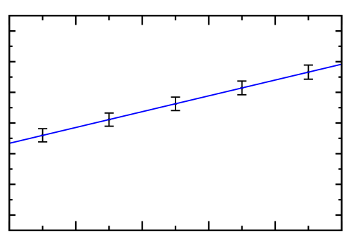
The results for $\langle m_{Bl}\rangle$ displayed in Tables 1 and 2 can be described by a linear function of the top quark mass. We present the results of such a fit for the two cases – with and without a cut on $m_{Bl}$ in Fig. 1. We find

$$\langle m_{Bl}\rangle^{\rm NLO}=0.601m_{t}-26.7~{}{\rm GeV},\;\;\;\delta_{\rm rms}=0.004;$$ (35)

$$\langle m_{Bl}\rangle_{m_{Bl}>50~{}{\rm GeV}}^{\rm NLO}=0.516m_{t}-0.96~{}{\rm GeV},\;\;\;\delta_{\rm rms}=0.006,$$ (36)

where $\delta_{\rm rms}$ is the root mean square (rms) of the residuals of the linear fit. It is clear from the value of $\delta_{\rm rms}$ that the linear fit works very well. It is straightforward to translate the results of the linear fit shown in Eqs. (35,36) to an estimate of the error on the top quark mass. Indeed, suppose that a typical uncertainty of the measured value of $\langle m_{Bl}\rangle$ is $0.4~{}{\rm GeV}$. The slopes in Eqs. (35,36) then imply that the corresponding error in the top quark mass $m_{t}$ is about $0.8~{}{\rm GeV}$. On the other hand, assuming perfect measurement of $\langle m_{Bl}\rangle$, we find that theoretical uncertainties in $\langle m_{Bl}\rangle$ shown in Table 1 and the value of the slope of the linear fit lead to a $1~{}{\rm GeV}$ uncertainty in the extracted value of the top quark mass. The errors on the top quark mass that follow from the NLO QCD computation are similar to differences between PYTHIA, HERWIG and NLO QCD. To show this, we quote results of a fit to $\langle m_{Bl}\rangle$ obtained with PYTHIA and HERWIG in Ref. [19]

$$\langle m_{Bl}\rangle_{\rm Pythia}=0.59~{}m_{t}-24.11~{}{\rm GeV},\;\;\;\;\langle m_{Bl}\rangle_{\rm Herwig}=0.61~{}m_{t}-25.31~{}{\rm GeV}.$$ (37)

It is clear from the comparison of the fits Eqs. (37,35) that NLO QCD results and parton shower results are close but not identical and these differences are essential. Indeed, we note that a slope difference between parton showers and NLO QCD is about $0.01$. Although such slope difference may look insignificant, it leads to ${\cal O}(3~{}{\rm GeV})$ shift in the reconstructed value of the top quark. Hence, parton showers are insufficient for measurements of the top quark mass with a precision higher than a few GeV. On the contrary, it follows from Eqs. (35,36) that NLO QCD computations lead to results with small uncertainties that can be estimated in a systematic way and, perhaps, be even further improved.

Figure 1: Results of the linear fit to $\langle m_{Bl}\rangle^{\rm NLO}$ are shown. Left panel – no cut on $m_{Bl}$ is applied. Right panel – $m_{Bl}>50~{}{\rm GeV}$ cut is applied. In both cases, decays of isolated top quarks are considered.

2.4 Results: $m_{Bl}$ distribution in $pp\to(t\to W^{+}+b\to W^{+}+B)+(\bar{t}\to W^{-}+\bar{b})$

In this Section, we consider production of $B$-mesons through the fragmentation of $b$-quarks in top decays but, in contrast to the previous Section, we include the full production process through next-to-leading order in perturbative QCD. To claim that the NLO QCD computation can do a good job in describing $\langle m_{Bl}\rangle$ in reality, it is very important to have full production and decay chain included.

To this end, we consider top quark pair production in $pp$ collisions at $\sqrt{s}=14~{}{\rm TeV}$ and focus on the lepton + jets decay channel. We note that NLO QCD corrections to the decay $W\to q\bar{q}^{\prime}$ need to be interfaced with $pp\to t\bar{t}$ production process, to describe lepton + jets channel through NLO QCD. We require that there are at least four jets in the event. We include the $B$-meson and the non-$B$-meson remnant of the fragmenting $b$-quark into a list of proto-jets that are passed to the jet reconstruction algorithm. We employ $k_{\perp}$ jet algorithm with $R=0.5$ and the four-momentum recombination scheme. All reconstructed jets and the positron from the $W^{+}$ decay are required to have transverse momenta in excess of $20~{}{\rm GeV}$. The scalar sum of the transverse momenta of all jets in the event should exceed $100~{}{\rm GeV}$ [20]. For the sake of simplicity, we do not impose any other kinematic constraints including cuts on the missing energy and the lepton isolation cuts. In addition, we do not consider combinatorial backgrounds, assuming that the correct pairing between a lepton and a $B$-meson can be established. Finally, similar to what was done in Ref. [13], throughout this paper we consider intermediate top quarks to be on the mass-shell and we do not include the so-called non-factorizable corrections [27]. For observables that we study in this paper, this is a good approximation since we, effectively, integrate over the invariant masses of each of the top quarks.

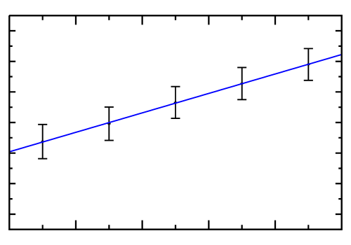
In contrast to the previous Section, we do not change the parameters of the fragmentation functions, fixing them to their central values, see Eq. (34). We use CTEQ parton distribution functions [28, 29] in the analysis. For each input value of $m_{t}$ we compute $\langle m_{Bl}\rangle$ for three values of the renormalization and (pdf)-factorization scales $\mu_{R}=\mu_{F}=[m_{t}/4,m_{t}/2,m_{t}]$ and for three values of the factorization scale in the $b\to B$ fragmentation function $[m_{t}/4,m_{t}/2,m_{t}]$ and for two different types of fragmentation functions Eq. (34). As the result, for each value of $m_{t}$ we have eighteen values of $\langle m_{Bl}\rangle$ and $\sigma_{m_{Bl}}$. Although this is not an extensive scan of the parameter space, it gives a sense of theoretical uncertainties in $\langle m_{Bl}\rangle$ provided that realistic production mechanism is employed. Computing the mean and the error, we arrive at the results shown in Table 3. We see that the NLO QCD effects in this case are quite small and negative, which is similar to the case of $m_{Bl}>50~{}{\rm GeV}$ cut discussed earlier. It is also clear that the uncertainty in $m_{Bl}$ decreases when NLO QCD corrections are included. By comparing results in Table 1 and in Table 3, we see that effects of kinematic cuts on $\langle m_{Bl}\rangle$ are more important at leading order, where the average value of $m_{Bl}$ can shift by $3.5~{}{\rm GeV}$. On the other hand, at NLO, a typical shift is of the order of $0.8~{}{\rm GeV}$ and, therefore, is less dramatic. Comparison of Tables 1 and 3 shows that the uncertainty of $\langle m_{Bl}\rangle$ at NLO nearly doubles if production mechanism is taken into account. Performing the fit, we obtain (see Fig.2)

$$\langle m_{Bl}\rangle^{\rm NLO}_{\rm prod}=0.6365~{}m_{t}-32.12~{}{\rm GeV},\;\;\;\delta_{\rm rms}=0.053.$$ (38)

Comparing this result with Eq. (35), we find a significant change in both the slope and the constant part. This demonstrates that $\langle m_{Bl}\rangle$ depends in a non-trivial way on the production mechanism, because of kinematic cuts applied to top quark decay products and additional jets in the production process. It follows from Eq. (38) and the uncertainties of $\langle m_{Bl}\rangle$ shown in Table 3 that the theoretical error on the extracted value of $m_{t}$ is close to $1.5~{}{\rm GeV}$.

$m_{t}$	$\langle m_{Bl}\rangle,\;{\rm LO}$	$\langle m_{Bl}\rangle,\;{\rm NLO}$	$\sigma_{m_{Bl}},\;{\rm LO}$	$\sigma_{m_{Bl}},\;{\rm NLO}$
$171$	$77.07\pm 1.92$	$76.75\pm 1.12$	$30.60\pm 0.13$	$28.41\pm 0.36$
$173$	$78.34\pm 1.93$	$77.92\pm 1.09$	$31.01\pm 0.14$	$28.72\pm 0.31$
$175$	$79.63\pm 1.98$	$79.31\pm 1.04$	$31.46\pm 0.14$	$29.12\pm 0.18$
$177$	$80.91\pm 2.03$	$80.55\pm 1.05$	$31.83\pm 0.15$	$29.48\pm 0.13$
$179$	$82.16\pm 2.04$	$81.80\pm 1.04$	$32.24\pm 0.16$	$29.83\pm 0.13$

Table 3: The average values of the invariant mass $\langle m_{Bl}\rangle$ and the dispersion in case where all the cuts on the final state particles are applied. The top quark masses and all the results are in GeV. See text for details.

Figure 2: Result of the linear fit to $\langle m_{Bl}\rangle^{\rm NLO}$ is shown, with all kinematic cuts on the final state particles applied. See text for details.

3 Dilepton channel

In the previous Section we saw that top quark decays to final states with identified hadrons provide an interesting way to determine the top quark mass. In this Section we study inclusive final states. We focus on the case where the top and the anti-top quarks decay semileptonically, e.g. $t\to W^{+}b\to l^{+}\nu b$. We study the kinematic distribution of an invariant mass of a $b$-jet and a lepton, and the distributions of the sum of energies of the two leptons and the two $b$-jets. We employ the NLO QCD corrections to top quark pair production and decay, as computed in Ref. [13]. Throughout this Section, the center-of-mass energy of proton collisions is $14~{}{\rm TeV}$.

We begin by summarizing the kinematic cuts that are employed to identify dilepton $t\bar{t}$ events [4]. Leptons are required to be central $|\eta^{l}|<2.5$ and have large transverse momentum $p_{\perp}^{l}>25~{}{\rm GeV}$. There should be missing energy in the event, $E_{\perp}^{\rm miss}>40~{}{\rm GeV}$. The jet transverse momentum cut is $p_{\perp,j}>25~{}{\rm GeV}$. We employ the $k_{\perp}$ jet algorithm with $R=0.4$.

3.1 Invariant mass of a lepton and a $b$-jet

It is pointed out in Ref. [4] that an average value of the invariant mass squared of a $b$-jet and a lepton $m_{lb}^{2}$ and an average value of the the angle between the lepton and the $b$-jet in the $W$ boson rest frame, can be used to construct an estimator of the top quark mass. The estimator reads

$$M_{\rm est}^{2}=m_{W}^{2}+\frac{2\langle m_{lb}^{2}\rangle}{1-\langle\cos\theta_{lb}\rangle}.$$ (39)

To see that this is a good estimator, we note that for the top quark decay computed at leading order in perturbative QCD and without any restrictions on the final state $M_{\rm est}$ equals to $m_{t}$

$$\langle m_{lb}^{2}\rangle=\frac{m_{t}^{2}-m_{W}^{2}}{2}\left(1-\langle\cos\theta_{lb}\rangle\right),\;\;\;\langle\cos\theta_{lb}\rangle=\frac{m_{W}^{2}}{m_{t}^{2}+2m_{W}^{2}}\;\;\;\;\Rightarrow M_{\rm est}^{2}=m_{t}^{2}.$$ (40)

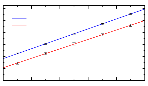
In reality $M_{\rm est}$ is not equal to $m_{t}$ for a variety of reasons including i) kinematic cuts required to identify the dilepton events; ii) effects of higher order QCD corrections; iii) impossibility to choose the “correct” pair of a lepton and a $b$-jet and iv) the experimental issues with $b$-jet misidentification and the jet energy resolution. The computation reported in Ref. [13] allows us to calculate $M_{\rm est}^{2}$ within the framework of perturbative QCD, accounting for the points i)-iii) exactly.

Figure 3: The invariant mass distribution of the lepton and the $b$-jet. Note that the lepton and the $b$-jet do not necessarily come from the decay of the same top quark, see text. The left panel shows the scale uncertainty bands for $\mu_{R}=\mu_{F}=[0.5m_{t},0.75m_{t},m_{t},1.25m_{t}]$. The right panel shows two NLO normalized $m_{lb}$ distributions for $m_{t}=171~{}{\rm GeV}$ and $m_{t}=179~{}{\rm GeV}$.

We point out that the computation of NLO QCD corrections to $pp\to t\bar{t}$ process reported in [13] includes exact spin correlations, one-loop effects in top quark decays and allows arbitrary constraints to be imposed on top quark decay products. These features are crucial for reproducing experimental procedures. Indeed, experimentally, it is not possible to determine the charge of the $b$-jet. Hence, it is unclear which of the two $b$-jets should be combined with the chosen, definite-sign, lepton. For the purpose of $m_{lb}$ reconstruction, one pairs the lepton with the $b$-jet that gives the smallest $m_{lb}$ value [4]. The parameter $\langle\cos\theta_{lb}\rangle$ in Eq. (39) is not measured and should be estimated theoretically. We have also chosen to calculate $\langle\cos\theta_{lb}\rangle$ for the $b$-jet that minimizes the invariant mass $m_{lb}$ since in this case, there is a partial compensation of incorrect assignments between the numerator and the denominator in Eq. (39). As the result, $M_{\rm est}$ becomes closer to the input value $m_{t}$ as compared to the case when “correct” pairing of the $b$-jet and the lepton is chosen to calculate $\langle\cos\theta_{lb}\rangle$ in Eq. (39). It is argued in Ref. [4] that with $10~{}{\rm fb}^{-1}$ integrated luminosity, the statistical and systematic uncertainties in the top quark mass of about $1~{}{\rm GeV}$ each can be achieved from $\langle m_{lb}^{2}\rangle$ measurement.

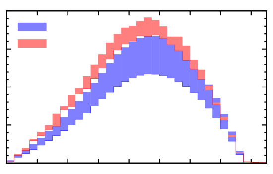
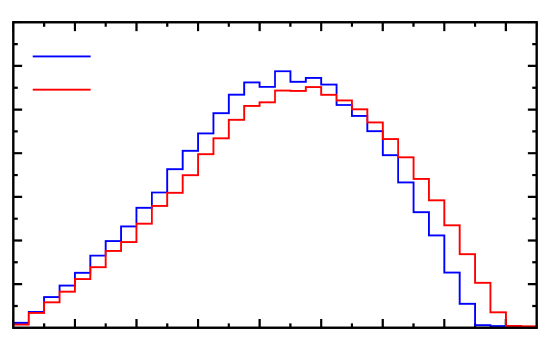
To assess how realistic those uncertainties are, we consider five different values of the top quark mass $m_{t}=[171,173,175,177,179]\;\;{\rm GeV}$. For each of these $m_{t}$ values, we compute $M_{\rm est}$ for four values of the renormalization and the factorization scales $\mu_{R}=\mu_{F}=[0.5m_{t},0.75m_{t},m_{t},1.25m_{t}]$ and for two sets of parton distribution functions CTEQ [28, 29] and MRST [30]. We use the mean value and the standard deviation of these eight values to compute central value of $M_{\rm est}$ and its error. Clearly, by no means this is an exhaustive scan through the parameter space but it gives us an idea of the uncertainties on the theoretical side. Examples of $m_{lb}$ distributions and the results of the calculation are shown in Figs. 3,4. The uncertainties on $M_{\rm est}$ do not depend on $m_{t}$ in significant way; they are $0.1~{}(0.2)~{}{\rm GeV}$ at leading and next-to-leading order, respectively. Performing the linear fit, we find

$$M_{\rm est}^{\rm LO}\;=\;0.8262m_{t}+23.22\;\mathrm{GeV},\;\;\;\;M_{\rm est}^{\rm NLO}=0.7850m_{t}+28.70\;\mathrm{GeV}.$$ (41)

The quality of the linear fit is very good; for example, the root mean square of the residuals of the NLO fit is $\delta_{\rm rms}=0.032$. It is instructive that the analysis of this observable at leading order shows stronger correlation between $m_{t}$ and $M_{\rm est}$ than at next-to-leading order. In addition, the theoretical uncertainty in $M_{\rm est}$ increases when NLO QCD corrections are included. The primary reason for the increased uncertainty is stronger dependence of $M_{\rm est}$ on the renormalization and factorization scales at NLO. This feature can be understood by considering the situation where no phase-space cuts are applied and where all the assignments of a lepton and a $b$-jet are done correctly. In this case, as follows from the discussion at the beginning of this Section, the estimator equals to the top quark mass regardless of the renormalization and factorization scales and the chosen parton distribution functions. At next-to-leading order, this is not true anymore because of the gluon radiation in top decay that is sensitive to the value of the strong coupling constant and, hence, to the renormalization scale. We note that we observe a very weak dependence of $M_{\rm est}$ on parton distribution functions which implies that even with the phase-space cuts and incorrect pairing, this variable is primarily sensitive to top quark decays rather than to top quark production mechanism.

Finally, we can use Eq. (41) and Fig. 4 to estimate uncertainty in $m_{t}$ that can be achieved by measuring $M_{\rm est}$ with infinite precision. Since, as follows from Fig. 4, the uncertainty in $M_{\rm est}$ is $0.2~{}{\rm GeV}$ at NLO and given the slope of about $0.8$ in Eq. (41), we find the minimal uncertainty in the extracted value of $m_{t}$ to be close to $0.25~{}{\rm GeV}$. We note that this result does not include the $b$-quark fragmentation uncertainty and the jet scale uncertainty, estimated to be $0.7$ and $0.6~{}{\rm GeV}$, respectively, in Ref. [4].

Figure 4: Results of a linear fit to $M_{\rm est}$, Eq. (39), at leading and next-to-leading order in perturbative QCD.

3.2 Sum of energies of the two leptons from top quark decays

Another observable that we consider is the sum of the energies of the two leptons, $E_{l_{1}}+E_{l_{2}}$, in the laboratory frame. Lepton energies in the laboratory frame can be easily measured and they are free from jet energy scale uncertainties that are important sources of errors, if the top quark mass is reconstructed from hadronic final states. The important question is whether or not the average value of the sum of lepton energies is correlated with the top quark mass at the parton level and how well such correlation can be described by perturbative QCD.

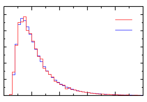
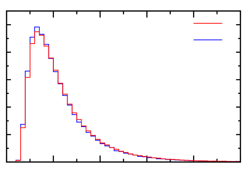
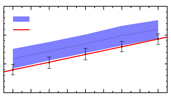
The corresponding distributions are shown in Fig. 5. There we display $E_{l_{1}}+E_{l_{2}}$ computed through leading and next-to-leading order in perturbative QCD for $m_{t}=175~{}{\rm GeV}$, as well the NLO QCD distributions in $E_{l_{1}}+E_{l_{2}}$ for $m_{t}=171$ GeV and $m_{t}=179~{}{\rm GeV}$. To compute the mean value of $\langle E_{l_{1}}+E_{l_{2}}\rangle$ we consider the same range of the renormalization and factorization scales and the two sets of parton distribution functions, as in the previous Section. The results of the calculation are shown in Fig. 6. Performing a linear fit, we find

$$\langle E_{l_{1}}+E_{l_{2}}\rangle_{\rm LO}\;\;=0.645m_{t}+120.6\;\mathrm{GeV},\;\;\;\;\delta_{\rm rms}=0.08;$$

$$\langle E_{l_{1}}+E_{l_{2}}\rangle_{\rm NLO}=0.670m_{t}+114.4\;\mathrm{GeV},\;\;\;\;\delta_{\rm rms}=0.07.$$ (42)

The results of the linear fit are displayed in Fig. 6. Theoretical errors on $\langle E_{l_{1}}+E_{l_{2}}\rangle$ are independent of the top mass; they are $1.7~{}{\rm GeV}$ at leading order and $1~{}{\rm GeV}$ at next-to-leading order. Combining information about the slope in Eq. (42) with the theoretical uncertainty on $\langle E_{l_{1}}+E_{l_{2}}\rangle$, we conclude that the ultimate uncertainty in $m_{t}$ that can be achieved by studying this observable is close to $1.5~{}{\rm GeV}$. It is interesting to point out that, in this case, both the scale dependence of the NLO result and the difference between MRST and CTEQ parton distribution functions are the two important sources of the uncertainty.

Figure 5: Left panel: normalized distribution of the sum of lepton energies at leading and next-to-leading order calculated for $m_{t}=175~{}{\rm GeV}$. The renormalization and factorization scales are set to $m_{t}$ and the MRST (left panel) and CTEQ (right panel) parton distribution functions set is used. Note a shift in the position of the maximum of this distribution. Right panel: normalized distributions of the sum of lepton energies at next-to-leading order, for $m_{t}=171~{}{\rm GeV}$ and $m_{t}=179~{}{\rm GeV}$.

Figure 6: Results of a linear fit to the sum of the average energy of the two leptons at leading and next-to-leading order.

3.3 Sum of jet energies

Another observable that was discussed [4] in connection with the top quark mass measurement is the sum of energies of the two hardest jets in the laboratory frame. Similar to the lepton energies just discussed, the shape of the distribution is an observable that is to be fitted; this is beyond the scope of the present paper. Here, we limit ourselves to the discussion of average values. Instead of considering the two hardest jets in the event, we found it more useful to take the sum of energies of the two $b$-jets.

Figure 7: Normalized distribution of the sum of energies of two $b$-jets $E_{\rm bjet}=E_{bj1}+E_{bj2}$ at next-to-leading order, calculated for $m_{t}=171~{}{\rm GeV}$ and $m_{t}=179~{}{\rm GeV}$. We set renormalization and factorization scales to $m_{t}$ and use CTEQ parton distribution functions.

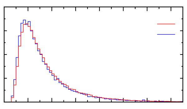
We consider the distribution of the sum of energies of the two $b$-jets. We expect that this distribution is strongly correlated with the top quark mass, since $b$-quarks originate directly from top decays. The results of the calculation are shown in Figs. 7. Performing a linear fit, we obtain the correlation between the average value of the two $b$-jets and the top quark mass

$$\langle E_{bj1}+E_{bj2}\rangle_{\rm LO}=2.18m_{t}-42.2\;\;{\rm GeV},\;\;\;\delta_{\rm rms}=0.02;$$

$$\langle E_{bj1}+E_{bj2}\rangle_{\rm NLO}=2.09m_{t}-29.2\;\;{\rm GeV},\;\;\;\delta_{\rm rms}=0.05.$$ (43)

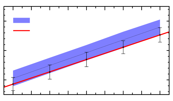
The results of the linear fit together with theoretical uncertainties in $\langle E_{bj1}+E_{bj2}\rangle$ are shown in Fig. 8. These uncertainties are $2.6~{}{\rm GeV}$ at LO and $2.4~{}{\rm GeV}$ at NLO; they do not exhibit a strong dependence on the top quark mass. Interestingly, inclusion of NLO QCD corrections makes the correlation between $\langle E_{bj1}+E_{bj2}\rangle_{\rm LO}$ and $m_{t}$ weaker. However, the correlation is still quite strong. If we assume that energies of $b$-jets can be measured infinitely accurately, the irreducible uncertainty on the determination of the top quark mass from $\langle E_{bj1}+E_{bj2}\rangle$ becomes only $1.2~{}{\rm GeV}$. Of course, the main issue here is to understand how well $b$-jet energies can actually be measured; this issue will be at the center of the experimental studies at the LHC.

Figure 8: Results of a linear fit to the sum of the average energy of the two $b$-jets at leading and next-to-leading order.

4 Conclusion

Determination of the top quark mass with high precision is an important part of the top quark physics program at the LHC. It is expected, that a variety of methods will be employed by ATLAS and CMS collaborations to measure the top quark mass. Some of those methods involve studies of the correlations between the value of the top quark mass and the kinematics of the top quark decay products. As the results of those studies, it is often claimed that the top quark mass can be determined with ${\cal O}(1\%)$ uncertainty at the LHC, but it is not clear whether or not these uncertainty estimates can be trusted. Indeed, all such studies employ PYTHIA or HERWIG parton shower event generators to describe top quark pair production and decay; however, no parton shower is designed to handle this level of precision. An interesting question therefore is to estimate, in a parton-shower-independent way, the uncertainty on $m_{t}$ that can be achieved in forthcoming LHC experiments.

The goal of this paper is to address this question by computing correlations between the top quark mass and the values of some kinematic observables through NLO QCD. Among other things, we consider NLO QCD corrections to the invariant mass of a $B$-meson and a lepton from top quark decays which is considered to be one of the most accurate ways to determine the top quark mass. Such computation is rather unusual in the context of NLO QCD calculations since it refers to the final state with an identified hadron.

In general, we find that parton shower event generators do a good job in estimating both the central value and the uncertainty in the top quark mass that can be achieved. However, as can be seen from the discussion of the average value of the invariant mass of the $B$-meson and the lepton, NLO QCD computations give both, a more accurate central values and an estimate of the uncertainty that can be trusted. Both of these features are important if we want to use the measured value of the top quark mass with confidence, to constrain physics beyond the Standard Model through precision measurements.

Acknowledgments K.M. would like to acknowledge conversations with A. Mitov that triggered this investigation and useful discussions with Z. Kunszt. This research is supported by the NSF under grant PHY-0855365 and by the start up funds provided by Johns Hopkins University. Calculations reported in this paper were performed on the Homewood High Performance Cluster of Johns Hopkins University.

References

- [1] T. Aaltonen et al. (The CDF Collaboration), Phys. Rev. D 81, 052001 (2010); Phys. Rev. D 81, 031102 (2010); Phys. Rev. D 80, 051104 (2009); Phys. Rev. D 79, 092005 (2009); Phys. Rev. D 79, 072001 (2009);
- [2] L. Brigliadori et al. (The CDF and D0 Collaboration) Nuovo Cim. C 032, 265 (2009); V.M. Abazov et al. (The D0 Collaboration), Phys. Rev. D 80, 092006 (2009)
- [3] ATLAS collaboration, “Expected performance of the ATLAS experiment: Detector, Trigger and Physics”, preprint CERN-OPEN-2008-20; CMS collaboration, “CMS Physics TDR: Physics Performance”, J. Phys. G: Nucl. Part. Phys. 34, 995 (2007).
- [4] M. Beneke et al., “Top quark physics,” arXiv:hep-ph/0003033.
- [5] D. Chakraborty, J. Konigsberg and D. Rainwater, Ann. Rev. Nucl. Part. Sci. 53, 301 (2003).
- [6] W. Wagner, Rept. Prog. Phys. 68, 2409 (2005).
- [7] A. Quadt, Eur. Phys. J. C 48, 835 (2006).
- [8] W. Bernreuther, J. Phys. G 35, 083001 (2008).
- [9] G. Corcella et al., JHEP 0101, 010 (2001).
- [10] T. Sjostrand, S. Mrenna and P. Skands, JHEP 0605, 036 (2006).
- [11] P. Nason, S. Dawson and R. K. Ellis, Nucl. Phys. B 327, 49 (1989) [ Erratum -ibid. B 335, 260 (1990)].
- [12] W. Beenakker, W.L. van Neerven, R. Menge, G.A. Schuler and J. Smith, Nucl. Phys. B 351, 507 (1991).
- [13] K. Melnikov and M. Schulze, JHEP 0908, 049 (2009).
- [14] W. Bernreuther and Z. Si, arXiv:1003.3926 [hep-ph].
- [15] J. M. Campbell and R.K. Ellis, Phys. Rev. D 62, 114012 (2000). The MCFM program is publicly available from http://mcfm.fnal.gov.
- [16] U. Langefeld, S. Moch and P. Uwer, Phys. Rev. D 80, 054009 (2009).
- [17] A. Kharchilava, Phys. Lett. B 476 (2000) 73.
- [18] G. Corcella, M.L. Mangano and M. H. Seymour, JHEP 0007, 004 (2000).
- [19] G. Corcella and F. Mescia, Eur. Phys. Journal C 65, 171 (2010).
- [20] R. Chierici, A. Dierlamm, CMS note 2006/058.
- [21] B. Mele and P. Nason, Phys. Lett. B 245, 635 (1990).
- [22] G. Corcella and A. D. Mitov, Nucl. Phys. B 623, 247 (2002)
- [23] S. Catani and M. H. Seymour, Nucl. Phys. B 485, 291 (1997) [Erratum-ibid. B 510, 503 (1998)].
- [24] J. M. Campbell, R. K. Ellis and F. Tramontano, Phys. Rev. D 70, 094012 (2004).
- [25] ALEPH Collaboration, A. Heister et al., Phys. Lett. B512, 30 (2001).
- [26] SLD Collaboration, K. Abe et al., Phys. Rev Lett. 84, 4300 (2000).
- [27] V.S. Fadin, V.A. Khoze and A.D. Martin, Phys. Rev. D 49, 2247 (1994); K. Melnikov and O.I. Yakovlev, Phys. Lett. B 324, 217 (1994); K. Melnikov and O.I. Yakovlev, Nucl. Phys. B 471, 90 (1996).
- [28] J. Pumplin, D. R. Stump, J. Huston, H. L. Lai, P. M. Nadolsky and W. K. Tung, JHEP 0207, 012 (2002).
- [29] P. M. Nadolsky et al., Phys. Rev. D 78, 013004 (2008).
- [30] A. D. Martin, R. G. Roberts, W. J. Stirling and R. S. Thorne, Eur. Phys. J. C 28, 455 (2003).