OUTP-1013P CERN-PH-TH/2010-127 Reconstructing events with missing transverse momentum at the LHC and its application to spin measurement
Abstract
In this article we discuss the measurement of spin at the LHC, in events with two unknown four-momenta. Central to this problem is the identification of spin-dependent kinematic variables and the construction of a statistical test that can distinguish between different spin hypotheses. We propose a method for reconstructing kinematic variables that depend upon the unknown momenta. The method is based upon a probabilistic reconstruction of each event, given the masses of the final and intermediate states and the cross-section of the assumed hypothesis. We demonstrate that this method can distinguish between two spin hypotheses for a specific process, even after mass uncertainties and Standard Model backgrounds are taken into account. We compare our method with another that only utilises the observable momenta of each event. We will show that our method permits an improved discrimination between hypotheses, with a reduced probability of error.
1 Introduction
Since the end of March 2010 high-energy collisions have been taking place at the Large Hadron Collider (LHC), ushering in a new era of particle physics. Over the coming decades the experiments at the LHC will test the Standard Model (SM) in a new energy regime and will search for the first conclusive evidence for physics beyond it. One possible signal for this new physics, which is motivated by the existence of dark matter, are events with large missing transverse momentum. Such events may have the following topology111In general, the event may also involve initial state radiation. We will assume that this can be neglected for the remainder of this paper.:
| (1) |
where constituents, , of the colliding protons interact to produce a pair of new particle states . These subsequently decay into an electrically neutral and colourless state (the DM candidate), that will escape detection, and a set of visible SM states . Because the four-momenta of the two particles are unknown, the kinematics of these events cannot be reconstructed. This loss of information will make it difficult to measure the masses, spins and couplings of these particle states. Such measurements, however, will be crucial if the physics underlying these signals is to be understood. In this paper we focus on the issue of spin measurement in events of this topology.
In order to determine the spin of either or , one must measure the probability density of some kinematic quantity. This distribution will then be compared to those predicted by several hypotheses, e.g. for different spin assignments to the particles in the event, and one must construct some statistical test in order to decide which hypothesis is correct. Central to this problem, therefore, is the identification of kinematic quantities, and an associated statistical test, that will permit a spin determination with a small probability of error. The ultimate goal is to identify an ‘optimal’ set, which will give the smallest probability of error for a fixed luminosity.
Previous studies of spin determination at the LHC have only considered kinematic quantities that are observable—i.e. those that can be uniquely determined for each event. Examples include Lorentz invariants formed from the visible momenta of decay products [1, 2, 3, 4, 5], and differences in pseudo-rapidities [6]. These variables, however, may not be optimal.
Alternative variables that depend upon the spin are the polar and azimuthal angles of production and decay, measured relative to some physical axis in the centre of mass frame and the rest frames of decaying particles. The energy dependence of the cross-section is another spin-dependent variable. It has been shown that using these variables one can determine the spin uniquely, in certain processes [7, 8, 9]. The difficulty with these variables is that they depend upon the unknown final state momenta, and so cannot be reconstructed event-by-event. This does not imply, however, that one cannot obtain some information regarding the probability density of these variables.
Consider some variable, , with probability density for some given hypothesis, . (In principle must specify all relevant physical quantities, including spins, masses and couplings.) It follows that:
| (2) |
where the sum is over each point, , in the phase space of the visible final state. Therefore, suppose we construct, for each hypothesis, the following distribution for a given set of events:
| (3) |
where the sum is over each of the events in the set. The conditional probabilities include all of the information that we have about an event, including the observed visible momenta and any information regarding the masses of and . If is the true hypothesis, this distribution will have the following form in the large statistics limit:
| (4) |
where the sum over events has been rearranged into a sum over phase space points, with the average number of events at the point . Since , it follows from Eqns. (2) and (4) that
| (5) |
In general, will tend to a different distribution if is a false hypothesis. Hence, in principal, one can identify the true hypothesis by comparing the distribution with . It is this idea that we will explore in this paper.
The remainder of this paper is organised as follows. In Sec. 2 we will demonstrate how one can construct, for a given hypothesis and kinematic variable, the distribution . We will then discuss how to construct a statistical test to compare different hypotheses and decide which is true.
In Sec. 3 we will apply our method to the discrimination of SUSY and UED models in slepton pair-production. For reference, we will compare our method with another that currently exists in the literature. We note that the purpose of this study is not to perform a fully rigorous analysis of how accurately our method will perform at the LHC. Such a study will require a full understanding of the detector and backgrounds, combined with a detailed study of systematic uncertainties. This is beyond the scope of this work. Rather, our goal is to perform a preliminary study, in a somewhat idealised case, in order to potentially identify the best method to use for a spin measurement.
Finally, in Sec. 4 we will summarise our results and make some suggestions for further developments.
2 The method
This section is composed of two parts. In the first we will discuss how to construct the distribution for a set of events and a given hypothesis . Then, in the second part, we will discuss how can be used in a statistical test to discriminate between different hypotheses.
2.1 Constructing
Let us consider a set of events with the topology of Eq. (1), where the initial and final state momenta are labelled as shown in Fig. 1. From this set we wish to construct the distribution , defined in Eq. (3), for some kinematic quantity and hypothesis . To do this we perform the following procedure. For each event, :
-
•
We determine the space of all possible four-momenta and that can be assigned to , consistent with the hypothesis . We will call this the space of solutions.
-
•
We construct the probability density on this space.
-
•
We integrate over the space of solutions to determine the distribution .
We then sum the from each event to obtain . We will now discuss each of these points in more detail.
2.1.1 The space of solutions
The final state of an event is parameterised by the eight unknown components of the two four-vectors and . Not all of these components are independent. Due to the conservation of four-momentum there exists the constraint:
| (6) |
where and are the (unknown) total energy and momentum, respectively, in the LAB frame. Hence the transverse components of and must satisfy:
| (7) |
We will further assume that the masses and , of the states and respectively, have been measured. Several methods have been proposed to measure these masses in a model independent manner, and we refer the reader to the relevant literature [10]. Hence, knowing the mass, one can apply the on-shell constraint to the unknown momenta:
| (8) |
The intermediate state will have some finite width, . It is unlikely that a reliable measure of will be possible at the LHC. Given this we will make the narrow width approximation for this state, which has the additional advantage of providing two further on-shell constraints:
| (9) |
Provided , this is likely to be a good approximation.
The six constraints given by Eqns. (7), (8) and (9) reduce the number of free parameters in the final state to two. Without loss of generality we choose these free parameters to be the transverse components . By solving the constraint equations one finds, for a given , two solutions for the four-momenta :
| (10) | ||||
| (11) | ||||
| (12) |
where . We have defined , where is the transverse mass of the four-vectors and :
| (13) |
and is the transverse energy. Through the substitutions and , with , one obtains the equivalent solutions for . For each choice of there are four discrete solutions, corresponding to the two different sign choices for and .
A real solution exists only if the two following constraints are satisfied: and . By choosing an orthogonal set of co-ordinate axes in the transverse plane such that , the first constraint can be written in the form:
| (14) |
where the constants and are given by:
| (15) | ||||
| (16) |
whilst the second has the form:
| (17) |
where
| (18) | ||||
| (19) |
Thus is constrained to lie within the overlap region of two ellipses, which are defined by Eqns. (14) and (17). Thus the space of solutions associated with an event is the set of four discrete solutions associated with each that lies within this overlap region.
2.1.2 Constructing a probability measure on the space of solutions
The probability measure is given by the differential cross-section:
| (20) |
where are the proton’s parton density functions (PDFs) and the sum is performed over all parton flavours . We define and such that:
| (21) | ||||
| (22) |
where is the beam energy. For the LHC we will assume the full design beam energy of 7 TeV.
The cross-section for the hard scatter is given by:
| (23) |
where is the total energy in the CM frame and a general four-momentum in the final state is written . The matrix element for the process, which is specified for a given hypothesis , is .
Making the narrow width approximation for the intermediate state forces to have the following structure:
| (24) |
where is a dimensionless quantity. Inserting Eq. (24) into Eq. (23) and integrating over the components of and , one finds, up to irrelevant constant factors:
| (25) |
where the sum over and corresponds to a sum over the solutions given in Eq. (12). The rapidity differences and are given by:
| (26) |
Hence the total differential cross-section has the form (again up to constant factors):
| (27) |
where and are fixed by the requirement:
| (28) | |||
| (29) |
Hence the probability measure is given by:
| (30) |
where correspond to the different and solutions at each point. The constant is defined such that .
2.1.3 Constructing
Given the space of solutions defined in Sec. 2.1.1 and the probability measure of Eq. (30), one can obtain the probability density for any kinematic quantity through a straightforward change of variables. In practice we simply integrate over the region of solution space for which takes a given value:
| (31) |
where the integral and sum is performed over the entire space of solutions.
2.2 The statistical test
The previous sections have detailed how to construct for a set of events. Given this distribution for each hypothesis, one would then like to decide which hypothesis is true. For this, we must construct a statistical test.
Since depends upon the random events in the set, is itself random and so will be distributed according to some probability density. For events distributed according to the hypothesis let us denote the probability density of as . (That is, is the probability density for in events generated and reconstructed with the same hypothesis. In statistics terminology, one can also consider to be a likelihood.) Let us assume that there are hypotheses , with , each with an associated probability density . If we knew each of these probability densities we could construct a statistical test as follows.
Suppose that we are given a set of events, and we are asked to determine which of the hypotheses is true. For each hypothesis we could calculate , as detailed above, and then calculate the associated probability, given the hypothesis, . We then reject the hypothesis in favour of if
| (32) |
where the constants are chosen so as to minimise errors (i.e. rejecting when is true, or accepting when is false). We will call the likelihood ratio.
Unfortunately we cannot calculate the probability densities analytically. Instead, they will be determined numerically, through Monte Carlo simulation. To simplify matters we will divide into discrete bins, where is made sufficiently small so as to simplify the calculation, without losing significant detail in the shape of . Thus for each set of events one calculates the discrete bin values , with . We will denote this set of values by the vector . Hence the problem of determining is reduced to finding the -dimensional probability distribution .
Since is the sum over many random variables:
| (33) |
one expects from the central limit theorem that it will have a Gaussian distribution. (This will hold provided . For any process that may be viably studied at the LHC one might expect , so this assumption seems reasonable.) It seems sensible therefore to assume an -dimensional Gaussian distribution for :
| (34) |
where is the average value in each bin and is the correlation matrix. In general, since is a smooth distribution, there will be significant correlations between the bin values. The parameters of this Gaussian distribution will be estimated using Monte Carlo simulation. We note, however, that it follows from the definition of that:
| (35) |
which provides an important cross-check of our method.
2.3 Summary
In this section we have discussed how one can construct and then use this in a statistical test to discriminate between hypotheses. In order to illustrate the method we apply it to an example in the following section.
3 A test of the method: Discriminating between models with different spin
| Model | ||||||
|---|---|---|---|---|---|---|
| SUSY | ||||||
| UED |
As a first test of the method we have attempted to discriminate between two models in the following process:
| (36) |
The models differ in their spin assignments and are based upon: supersymmetry (SUSY), where is the scalar superpartner of the muon and is a Majorana fermion, and universal extra dimensions (UED), where and are the first Kaluza-Klein excitation of the muon and gauge boson, respectively. The spin and representation under the SM gauge group of and are summarised for each model in Table 1.
Several previous works have shown that a (partial) measurement of the spin of is feasible in this process, both at a linear collider and at the LHC [8, 6, 9]. Let us summarise, briefly, how this can be achieved.
The initial state of this process is forced to have a total angular momentum . (This is a consequence of the antiparallel momenta of the and together with their coupling to an s-channel vector boson.) Hence, in the SUSY model, the scalar pair must be produced in a -wave state, in order to conserve angular momentum. These states carry orbital angular momentum and have a non-trivial angular distribution. Thus the SUSY matrix element has the form:
| (37) |
where and are the polar angle of the momentum, measured relative to the beam-line, and the speed of , as observed in the CM frame. The factor is dimensionless and independent of . This matrix element vanishes in the limits and as a straightforward consequence of angular momentum conservation. If, however, carries intrinsic angular momentum through a non-zero spin, total angular momentum can be conserved even with vanishing orbital angular momentum. Hence the can be produced in an -wave state, which has a matrix element that is non-zero for all and . The precise form of the matrix element depends upon the spin and couplings of . If is spin-1/2 with vector-like couplings, as in UED, this matrix element has the form:
| (38) |
Thus the distributions of both and are sensitive to the spin and can be used to discriminate between the SUSY and UED models. A more general analysis has shown that for a process of this kind, these distributions are sufficient to discriminate between the hypotheses and [8].
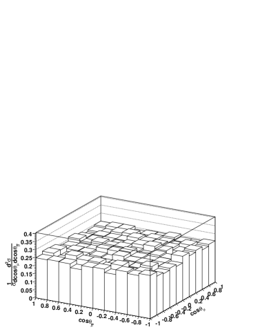
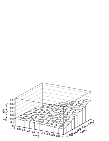
Other variables are also sensitive to the spin, such as the azimuthal and polar angles of the () momenta in the rest frame of the (). Of particular interest are the following:
-
•
The azimuthal angle between the decay planes of the and , defined in the CM frame. As pointed out in [9], has a distribution of the form:
(39) Hence one can infer the spin of from the highest component of the distribution.
-
•
The polar angles () of the (), measured in the rest frame of the (). These are measured relative to the direction of the boost from the LAB to the CM frame, as viewed in the appropriate rest frame. In the rest frame of only its polarisation can break rotational invariance. Hence the observation of a non-trivial distribution in and indicates that must be polarised and hence have a non-zero spin. For the UED model there is a large correlation222This correlation arises because the decay vertex involves a chiral coupling and there is a net polarisation of the initial state along the direction of the boost, , from the CM frame to the LAB frame. This polarisation arises as follows. Because is a doublet under the process involves a significant contribution from s-channel exchange. Since the has chiral couplings to the quarks, this results in an overall polarisation of the initial state along the direction defined by the incoming quark’s momentum. However, owing to the structure of the pdfs and the mass of , this direction is correlated with the direction of the boost . between these angles, whilst the SUSY distribution is flat, as shown in Fig. 2.
Unfortunately, all of these variables depend upon the unknown momenta, so they cannot be uniquely determined for an event at the LHC. However, we propose to employ our method to reconstruct their distributions and so discriminate between models.
An alternative method has been proposed for use at the LHC, which depends upon the variable [6]:
| (40) |
where is the pseudorapidity difference between the and . This variable depends only upon the observable momenta and so is straightforward to reconstruct. Because it depends upon a pseudorapidity difference, it is invariant under longitudinal boosts and so is sensitive to the direction of the system in the CM frame. Since these states tend to be boosted in the direction of their parent and this variable is correlated with the polar angle , and so is sensitive to the spin. We propose to use this method as a benchmark for our own.
3.1 Simulating events at the LHC - signal, background and event selection
The LHC experiments will search for events from this process using the signature of two opposite sign muons, in association with missing transverse energy. There will, however, be significant background sources of such events arising from SM processes.
A realistic test of our method must take into account the effect of these backgrounds. However, a complete background analysis, combined with detector effects and associated systematic errors is far beyond the scope of this work. Instead we will perform our test only at parton level, without hadronisation and detector simulation. Furthermore, we will only include a limited number of backgrounds in this analysis. Previous studies [6] have identified several important sources, the most important of which is the irreducible SM background:
| (41) |
This is the only one that we will take into account333Using the cuts listed below, it has been found [6] that this process accounts for over of the background signal.. Despite these simplifications this test should still establish whether, in principal, our method improves upon the use of the distribution.
In order to isolate the signal events from background we follow the work of Barr [6] and apply the following selection criteria:
-
•
The transverse momenta of the muons must satisfy and , where, by definition, .
-
•
The invariant mass of the muon pair must satisfy:
-
•
The missing transverse energy must satisfy
-
•
where the kinematic variable [11, 12] is defined as:
| (42) |
where the minimisation is subject to the constraints and . These cuts have been developed to eliminate most of the events from the SM di-boson processes: and production, but have not been tuned to maximise the ratio of signal to background. In addition to these criteria we also demand that the final state muons have a pseudorapidity , which is required to ensure a high reconstruction efficiency in both ATLAS and CMS [13, 14].
Using MadGraph/MadEvent [15] we find that the leading order cross-section for the SM process given in Eq. (41) is, after applying the above cuts,
| (43) |
The signal events for both the SUSY and UED model were also generated using MadGraph/MadEvent. The UED model was implemented as a user-defined model, with particle widths calculated using the program BRIDGE [16]. For this test we fixed the masses at and . For the SUSY model we found a leading order cross-section, after cuts, of
| (44) |
whilst the cross-section for the UED model takes a significantly larger value. Because the couplings of the new particle states cannot be known prior to a spin determination, the cross-section cannot be used as true spin (or model) discriminant. (Our method only relies upon the shape of the distributions to perform the discrimination.) Thus we simulate both SUSY and UED models by assuming the same cross-section for each and, to be conservative, we choose the smaller cross-section of the SUSY model.
3.2 Implementing and testing our method
For this test we performed a total of 2000 pseudo-experiments, each with a total integrated luminosity , for each model. In each pseudo-experiment the number of signal and background events were selected at random from Poisson distributions with means and , respectively. The corresponding number of signal and background events were then generated and reconstructed using our method.
When calculating for each hypothesis we made several simplifications in the probability measure , given in Eq. (30). Rather than use the full matrix element for either hypothesis, we instead used the matrix element for the production process only, which are given in Eqns. (37) and (38). The factors were treated as dimensionless constants and were absorbed into the normalisation factor . In addition, we only include the PDFs for the up-type quarks444We have found that there is no significant difference between using the PDFs for either the up-type or down-type quarks., which were calculated using the NNLO central MSTW set [17], at a scale . These approximations were motivated by the desire to lessen the dependence of the reconstruction on unknown, mode-dependent factors, such as the structure of decay vertices and the strengths of couplings. With these approximations we are effectively left with with a probability measure that is independent of these unknown factors. The approximations neglect some very mild dependence on that is actually present in the factors, and spin correlations in the decays of are also neglected.
Because the number of signal and background events expected to pass the selection criteria are comparable, the reconstructed distribution will contain a significant background contamination. A background subtraction was performed in order to isolate the signal contribution to . To do this we determined the average background contribution, , which was then subtracted in each pseudo-experiment to obtain a new distribution:
| (45) |
These subtracted distributions were then used to perform the statistical tests discussed in Sec. 2.2. In particular, they were used to determine the means and the covariance matrix for the probability densities and , using unbiased estimators. These probability densities were then used to calculate, for each pseudo-experiment, the likelihood ratio
| (46) |
3.3 Results
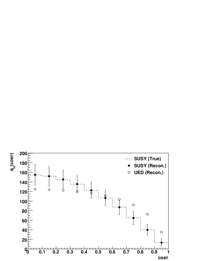
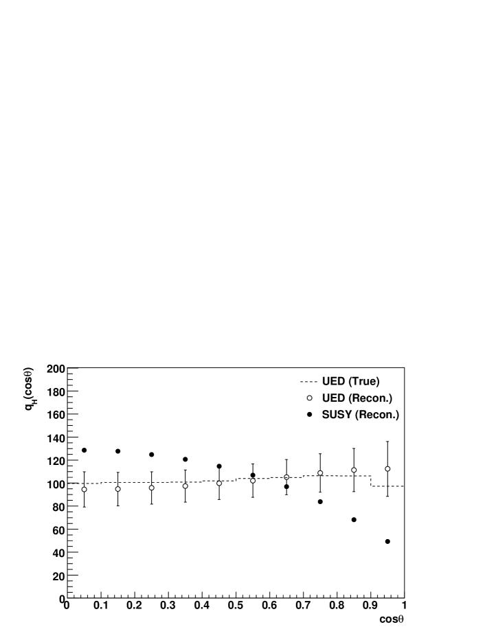
To begin, we will discuss our results from an attempt to reconstruct the distribution, which we divided into bins. To perform the reconstruction we assumed masses and , where and are the true (pole) masses of and , respectively, that were used to generate the events. In Sec. 3.3.1 we will discuss the effect of errors in these assumed masses.
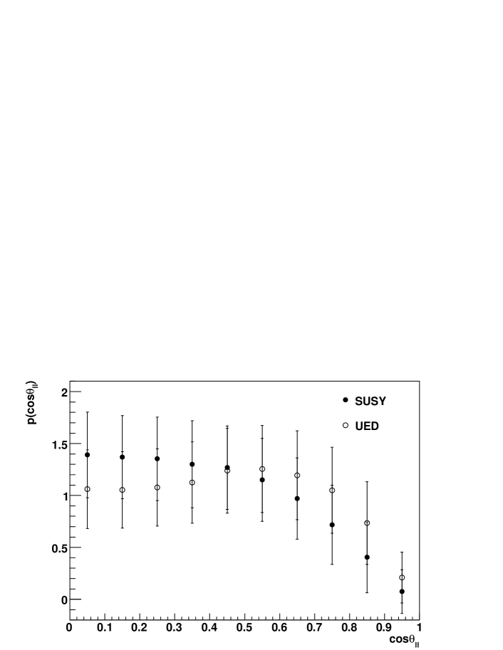
In Fig. 3(a) and Fig. 3(b) we show the average distribution for and , respectively. In each plot we show the distribution obtained from events generated for the SUSY model (filled circles) and UED model (open circles). The histogram in each plot shows the distribution. Also shown in each plot are error bars, where the error in the bin is given by the corresponding estimated variance:
| (47) |
It can be seen from these figures that events reconstructed with the true hypothesis have a distribution that is in agreement with . This is as we expected, and provides an important validation of our method. However, we observe that there is a small discrepancy for events from the UED model. We expect that this is caused by our neglect of spin-correlations in the reconstruction, as discussed in Sec. 3.2.

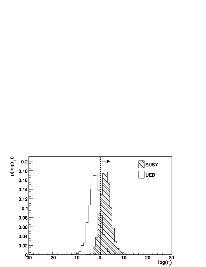
Crucially, we observe that there is a significant discrepancy between events from the SUSY and UED models when reconstructed with the same hypothesis. This demonstrates that the method can discriminate between the two models, at least in principal. In Fig. 4 we show a plot of the distribution for events from SUSY (hatched histogram) and UED (empty histogram). The SUSY and UED distributions are well separated, thus indicating that is a potentially useful test statistic. To define our statistical test we choose our acceptance region, in which we accept the SUSY hypothesis instead of UED, as:
| (48) |
From the distribution of Fig. 4 this test is expected to have a significance555The significance of a hypothesis test is defined as the probability of an error of the first kind, i.e. the probability of rejecting the hypothesis of SUSY, if SUSY is the true hypothesis [18].:
| (49) |
and power666The power of a hypothesis test to discriminate between the hypotheses is given by , where is the probability of an error of the second kind, i.e. the probability of accepting the hypothesis of SUSY when SUSY is false [18].:
| (50) |
To put this result into context we compared this with a test based upon the distribution. In Fig. 5(a) we show the average distribution for our sample of 2000 pseudo-experiments, for both SUSY and UED models, after the average SM background contribution has been subtracted.
We constructed a statistical test for this method as follows. We assumed, for each hypothesis , that the number of events in the bin, after subtraction of the averaged background, is a Gaussian random variable with a mean and variance that were estimated from the set of pseudo-experiments. Using these Gaussian distributions we calculated for each pseudo-experiment the likelihood ratio
| (51) | ||||
| (52) |
The distribution of is shown for both SUSY and UED models in Fig. 5(b). The SUSY and UED distributions are separated, however there is a significant overlap between the two. If we define the acceptance region as:
| (53) |
we find a statistical test with acceptance and power . Comparing this with Eqns. (49) and (50) we find that our method reduces the probability of error by a factor of .


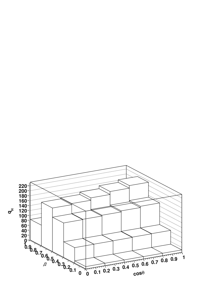
Following this initial test we attempted to improve our model discrimination by including additional kinematic variables. In Fig. 6 we show the joint distribution for the SUSY events, reconstructed with both hypotheses after the average background has been subtracted. The distribution for the UED events is shown in Fig. 7. One interesting feature of these distributions is that the dependence is insensitive to the hypothesis used in the reconstruction. As can be observed in Fig. 6 the distribution for the SUSY events is peaked closer to 1 than in the UED events, as one would expect given the dependence of the matrix elements. Following the same procedure as before we constructed the probability distributions , and determined the likelihood ratio for each experiment. This distribution is given in Fig. 8 for both SUSY and UED events.

Comparing Fig. 8 and Fig. 4 one can see that by combining both and it is possible to enhance the separation of the SUSY and UED events, compared to reconstructing alone. Defining the acceptance region for the SUSY hypothesis as:
| (54) |
we obtain a statistical test with significance and power . This test improves over using alone by a factor of , and is over 10 times less likely to result in error than the method.
Attempts to further improve the hypothesis test by including the kinematic variables , and were unsuccessful. Although our method could reconstruct some features of these distributions they were not statistically significant once the background contribution was taken into account.
3.3.1 The effect of mass uncertainties
Errors in the measurement of the masses and will affect the efficacy of our proposed statistical tests. To study the effect of such a systematic error we varied the true mass , used to generate the events, whilst keeping our statistical test fixed. (That is, the masses assumed for the reconstruction were fixed at and , and we used the same probability densities and acceptance region defined in the previous section.) Assuming an uncertainty in the mass , we performed another 2000 pseudo-experiments for the cases and . For each case, the significance and power of each statistical test is given in Table 2.
We observe that the tests based upon the and distributions are quite insensitive to the 10% mass uncertainty, with variations in and at the level of 10—50%. Thus these tests, at least, are fairly robust against uncertainties in the mass measurement. However, the test based upon exhibits a much larger variation with and . This large variation appears to be caused by the sensivity of the distribution to the true and assumed masses. Hence, a 10% mass uncertainty reduces the significance and power of this test, causing it to be less effective than the test based upon .
| Variable | Acceptance Region | ||||||
|---|---|---|---|---|---|---|---|
| 3.3% | 98.3% | 3.3% | 96.1% | 4.7% | 98.5% | ||
| , | 1.2% | 99.1% | 2.8% | 99.7% | 0.5% | 95.2% | |
| 14.8% | 84.9% | 12.3% | 84.6% | 15.3% | 82.7% | ||
4 Conclusions
In this paper we have proposed a new method for reconstructing the probability distributions of kinematic variables that are sensitive to the spin of new particle states. This method relies on performing a probabilistic reconstruction of each event, combining information from the measured particle masses and the matrix element for a hypothesised process. As a result, one is able to study kinematic observables that depend on unknown momenta, such as that carried by two potential DM candidates. By combining the information from a sample of events we have shown how one can attempt to reconstruct this probability distribution and then test the assumed hypothesis.
We have performed a preliminary test of the method on a candidate process: the discrimination of SUSY and UED models in slepton-pair production. This test was performed at parton level, without hadronisation or detector simulation, and took into account the effects of event selection and the dominant SM backgrounds. We have shown that with 100 of luminosity one can discriminate between the SUSY and UED models, with a probability of error of . This result has been shown to be robust against a 10% uncertainty in the mass measurement. Our complete results are summarised in Table 2 and show that, in principle, one can improve the test by combining several independent variables. However, the improvement gained in practice will depend upon the uncertainty in the masses.
We compared this result with that expected for an alternative method, which uses the variable . We find, for the process considered, that this can perform a discrimination with a probability of error of . Thus, potentially, our method offers an improved way of discriminating between models and measuring the spin.
Despite this encouraging result, many further questions remain and deserve detailed study. The true efficacy of our method can only be understood through a real world application, together with more detailed simulation. In particular, it will be crucial to study the effect of systematic uncertainties in the background estimation and mass measurement, combined with the effects of detector resolution and acceptance. Furthermore, it would be of interest to study how this method performs in a wider range of processes. Possible processes of interest are those that involve long decay chains, or those involving diagrams with both s- and t-channel particle exchange.
Acknowledgements
DH would like to thank Graham G. Ross for several enlightening discussions and comments on the manuscript. Further thanks also go to Alan J. Barr, for useful insights on experimental matters related to event selection and simulation. This research project has been supported by a Marie Curie Early Initial Training Network Fellowship of the European Community’s Seventh Framework Programme under contract number (PITN-GA-2008-237920-UNILHC).
References
- [1] C. Athanasiou, C. G. Lester, J. M. Smillie, B. R. Webber, Distinguishing spins in decay chains at the Large Hadron Collider, JHEP 08 (2006) 055.
- [2] A. J. Barr, Using lepton charge asymmetry to investigate the spin of supersymmetric particles at the LHC, Phys. Lett. B596 (2004) 205–212.
- [3] L.-T. Wang, I. Yavin, Spin Measurements in Cascade Decays at the LHC, JHEP 04 (2007) 032.
- [4] M. Burns, K. Kong, K. T. Matchev, M. Park, A General Method for Model-Independent Measurements of Particle Spins, Couplings and Mixing Angles in Cascade Decays with Missing Energy at Hadron Colliders, JHEP 10 (2008) 081.
- [5] M. Kramer, E. Popenda, M. Spira, P. M. Zerwas, Gluino Polarization at the LHC, Phys. Rev. D80 (2009) 055002.
- [6] A. J. Barr, Measuring slepton spin at the LHC, JHEP 02 (2006) 042.
- [7] F. Boudjema, R. K. Singh, A model independent spin analysis of fundamental particles using azimuthal asymmetries, JHEP 07 (2009) 028.
- [8] S. Y. Choi, K. Hagiwara, H. U. Martyn, K. Mawatari, P. M. Zerwas, Spin analysis of supersymmetric particles, Eur. Phys. J. C51 (2007) 753–774.
- [9] M. R. Buckley, S. Y. Choi, K. Mawatari, H. Murayama, Determining Spin through Quantum Azimuthal-Angle Correlations, Phys. Lett. B672 (2009) 275–279.
- [10] A. J. Barr, C. G. Lester, A Review of the Mass Measurement Techniques proposed for the Large Hadron Collider.
- [11] C. G. Lester, D. J. Summers, Measuring masses of semiinvisibly decaying particles pair produced at hadron colliders, Phys. Lett. B463 (1999) 99–103.
- [12] A. Barr, C. Lester, P. Stephens, m(T2) : The Truth behind the glamour, J. Phys. G29 (2003) 2343–2363.
- [13] G. Aad, et al., Expected Performance of the ATLAS Experiment - Detector, Trigger and Physics.
- [14] D. Acosta, M. Della Negra, L. Foà, A. Hervé, A. Petrilli, CMS physics: Technical Design Report, Technical Design Report CMS, CERN, Geneva, 2006.
- [15] J. Alwall, et al., MadGraph/MadEvent v4: The New Web Generation, JHEP 09 (2007) 028.
- [16] P. Meade, M. Reece, BRIDGE: Branching ratio inquiry / decay generated events.
- [17] A. D. Martin, W. J. Stirling, R. S. Thorne, G. Watt, Parton distributions for the LHC, Eur. Phys. J. C63 (2009) 189–285.
- [18] G. Cowan, Statistical data analysis, Oxford University Press, Oxford, UK, 1998.