Modeling and Simulation of Liquid Crystal Elastomers

Abstract

We consider a continuum model describing the dynamic behavior of nematic liquid crystal elastomers (LCEs) and implement a numerical scheme to solve the governing equations. In the model, the Helmholtz free energy and Rayleigh dissipation are used, within a Lagrangian framework, to obtain the equations of motion. The free energy consists of both elastic and liquid crystalline contributions, each of which is a function of the material displacement and the orientational order parameter. The model gives dynamics for the material displacement, the scalar order parameter and the nematic director, the latter two of which correspond to the orientational order parameter tensor. Our simulations are carried out by solving the governing equations using an implicit-explicit scheme and the Chebyshev polynomial method. The simulations show that the model can successfully capture the shape changing dynamics of LCEs that have been observed in experiments, and also track the evolution of the order parameter tensor.

1 Introduction

Liquid crystal elastomers (LCEs) are orientationally ordered solids, combining features of liquid crystals and elastic solids.  They were first proposed by de Gennes [5] and first synthesized by Finkelmann et al [8].  They consist of weakly cross-linked liquid crystal polymers with orientationally ordered side or main-chain mesogenic units. They exhibit many new phenomena not found in either liquid crystals or polymers.  The salient feature of LCEs is the strong coupling between mechanical deformation and orientational order. As a consequence of this coupling, mechanical strains change the order parameter and hence physical properties of LCEs, and, conversely, extermal stimuli, such as light, affecting orientational order can produce large shape changes [2, 13, 18, 20].

Although many fascinating experimental results have been obtained studying the dynamic response of LCEs to external stimuli [3, 4, 9, 13, 14, 17, 21, 20], their dynamics is not fully understood. In this paper, we implement a non-local continuum model [7], chose and explicitly define a specific representation and carry out numerical simulations to explore the dynamic behavior.  Our work thus includes both components of modeling and simulation.

In the model, the Helmholtz free energy and Rayleigh dissipation are combined, using a Lagrangian approach, to obtain the dynamics.  The free energy consists of both elastic and nematic contributions, and includes volume conservation. As a special case of the continuum model, we choose a simple local form of the nematic free energy, the Maier-Sauper free energy, to describe nematic contributions. Our model considers only the uniaxial phase of nematic LCEs, for which the order parameter tensor can be expressed in terms of a scalar order parameter and nematic director; direct contributions to the free energy from spatial variations of the order parameter and director are neglected. These simplifications make our model more tractable both theoretically and numerically.  Subsequently, the governing equations can be derived explicitly using both conserved and non-conserved order parameter dynamics. We thus obtain the time dependent equations for the displacement, scalar order parameter and nematic director.

The equations obtained are more complicated than the standard Navier-Stokes equations in the Eulerian frame. First, besides the pressure term and the viscous term, there is also an elastic term in the velocity equation.  Second, our equations are written in a Lagrangian frame. This choice is straightforward for capturing the orbit as well as the dynamics of each particle in the LCE sample. Indeed, Eulerian coordinates are not well suited to our problem since the domain occupied by the LCE sample varies in time.  Moreover, the derived velocity equation is very stiff due to the presence of different time scales in the problem, posing challenges for the simulation. The simulation is therefore a fascinating but a very formidable problem.  In this work, we employ the Chebyshev polynomial method [15] to discretize the spatial derivatives in the dynamical equations. This method, as a typical spectral method, can achieve high accuracy, and is particularly well suited to our simulation as our system is non-periodic. We also apply the popular implicit-explicit (IMEX) schemes for the time-discretization of the equations.  Specifically, a combination of second-order Adams-Bashforth method for explicit terms and Crank-Nicolson method for implicit terms [1, 10, 15] are used.

The paper is organized as follows. In Section 2, we give the details of the model as well as the derivation of the governing equations. To obtain the equations, we first calculate the functional derives of those functionals with respect to the principal variables, i.e., material displacement, order parameter and nematic director, and then apply the appropriate conserved/non-conserved dynamics for each of the variables. In Section 3, we present the numerics for solving the equations and then show the results of our simulations. Conclusions are given in Section 4.

2 Modeling nematic LCEs

To describe the dynamics of LCEs, in addition to orientational order, one needs to track the time evolution of the position of the crosslinks of the LCE network. In the case of uniaxial nematic LCEs, the sample can be characterized by the displacement, order parameter and nematic direction at each Lagrangian lattice site, corresponding to a cross-link.  Our work is to study how these key variables evolve in time when the sample is subjected to external stimuli.  To this end, we represent the continuum model in terms of these variables, derive the governing equations and implement the simulation by solving the equations numerically.

Our continuum model consists of the elastic free energy density and the nematic free energy density with coupling between orientational order and deformation of the network, a Rayleigh dissipation function and a volume preserving functional. The governing equations are derived from these by applying the appropriate dynamics for each key variable. In what follows, the functionals and the functional derivatives are discussed.

2.1 Energy functionals

The free energy in our model is composed of elastic and nematic contributions. The elastic free energy describes the nonlocal interaction between connected cross-links of elastomers, while the nematic free energy represents the anisotropic dispersion interactions of the mesogenic constituents.

2.1.1 The elastic free energy

Let $\alpha$ denote a material point in the LCEs sample, and $\mathbf{x}(\mbox{{\boldmath$\alpha$}},t)$ the location of the point $\alpha$ at time $t$. To describe the nematic ordering in the LCEs crossing-link network, an effective dimensionless step length tensor $\mathbf{L}$ is introduced, being written as $\mathbf{L}=\mathbf{I}+2\mu\mathbf{Q}$, where $\mathbf{Q}$ is the orientational order parameter tensor, $\mathbf{I}$ is the identity matrix and $\mu$ is the relaxation parameter. In the uniaxial phase case, $\mathbf{Q}=S(\frac{3}{2}\mathbf{n}\mathbf{n}^{T}-\frac{1}{2}\mathbf{I})$, where $\mathbf{n}$ represents the unit vector along the average alignment direction of the molecular symmetry axes, $S$ is the scalar order parameter describing the degree of alignment of the molecular axes with $\mathbf{n}$ [6].

In the undeformed state, the probability density of finding in the LCEs sample a polymer chain of length $\mathcal{L}$ starting at $\alpha$ and ending at $\mbox{{\boldmath$\alpha$}}^{\prime}$ can be written as

$$P_{0}(\mbox{{\boldmath$\alpha$}},\mbox{{\boldmath$\alpha$}}^{\prime})=(\frac{3}{2\pi\mathcal{L}b})^{3/2}(\det\mathbf{L}_{0})^{-1/2}\exp\left(-\frac{3(\mbox{{\boldmath$\alpha$}}^{\prime}-\mbox{{\boldmath$\alpha$}})^{T}\mathbf{L}_{0}^{-1}(\mbox{{\boldmath$\alpha$}}^{\prime}-\mbox{{\boldmath$\alpha$}})}{2\mathcal{L}b}\right),$$

where $\mathbf{L}_{0}=\mathbf{I}+2\mu\mathbf{Q}_{0}$ is the effective step length at the initial state [18].  Since $\mathbf{Q}_{0}$ is assumed to be slowly varying compared to the distance between crosslinks, we evaluate $\mathbf{Q}_{0}\mathbf{\,}$ and $\mathbf{L}_{0}$ at position $\alpha$.

At time $t$, the probability density of finding a polymer ending at $\mathbf{x}(\mbox{{\boldmath$\alpha$}},t)$ and $\mathbf{x}(\mbox{{\boldmath$\alpha$}}^{\prime},t)$ shares the same form as $P_{0}(\mbox{{\boldmath$\alpha$}},\mbox{{\boldmath$\alpha$}}^{\prime})$ with $\mathbf{L}_{0}(\mbox{{\boldmath$\alpha$}})$ being replaced by $\mathbf{L}(\mbox{{\boldmath$\alpha$}},t)$. The free energy of the particular polymer initially ending at $\alpha$ and $\mbox{{\boldmath$\alpha$}}^{\prime}$ is $-kT\ln[P(\mathbf{x}(\mbox{{\boldmath$\alpha$}},t),\mathbf{x}(\mbox{{\boldmath$\alpha$}}^{\prime},t))]$, where $k$ is the Boltzmann’s constant, $T$ is the temperature.  The total elastic free energy at time $t$ is

$$F_{el} =\frac{1}{2}\int d^{3}\mbox{{\boldmath$\alpha$}}\mathcal{F}_{el}$$

$$=\frac{1}{2}\int d^{3}\mbox{{\boldmath$\alpha$}}\int d^{3}\mbox{{\boldmath$\alpha$}}^{\prime}\rho_{c}P_{0}(\mbox{{\boldmath$\alpha$}},\mbox{{\boldmath$\alpha$}}^{\prime})\Bigl{(}-kT\ln[P(\mathbf{x}(\mbox{{\boldmath$\alpha$}},t),\mathbf{x}(\mbox{{\boldmath$\alpha$}}^{\prime},t))]\Bigr{)}$$

$$=\int d^{3}\mbox{{\boldmath$\alpha$}}\int d^{3}\mbox{{\boldmath$\alpha$}}^{\prime}H(\mbox{{\boldmath$\alpha$}},\mbox{{\boldmath$\alpha$}}^{\prime})\Bigl{(}\frac{3}{2\mathcal{L}b}(\mathbf{x}(\mbox{{\boldmath$\alpha$}}^{\prime},t)-\mathbf{x}(\mbox{{\boldmath$\alpha$}},t))^{T}\mathbf{L}^{-1}(\mathbf{x}(\mbox{{\boldmath$\alpha$}}^{\prime},t)-\mathbf{x}(\mbox{{\boldmath$\alpha$}},t))$$

$$+\frac{1}{2}\ln\det\mathbf{L}\Bigr{)},$$ (1)

where$~{}\mathcal{F}_{el}$ is the elastic free energy density,

$$H(\mbox{{\boldmath$\alpha$}},\mbox{{\boldmath$\alpha$}}^{\prime})=(\frac{1}{2}\rho_{c}kT)(\frac{3}{2\pi\mathcal{L}b})^{3/2}(\det\mathbf{L}_{0})^{-1/2}\exp\left(-\frac{3(\mbox{{\boldmath$\alpha$}}^{\prime}-\mbox{{\boldmath$\alpha$}})^{T}\mathbf{L}_{0}^{-1}(\mbox{{\boldmath$\alpha$}}^{\prime}-\mbox{{\boldmath$\alpha$}})}{2\mathcal{L}b}\right),$$

and $\rho_{c}$ is the number density of crosslinks.

2.1.2 Nematic free energy

Perhaps the most successful description of nematic order is Maier-Saupe theory.  Here, the single particle potential is

$$\mathcal{E}=-U\rho_{lc}SP_{2}(\cos\theta)+\frac{1}{2}U\rho_{lc}S^{2},$$

where $U$ is an interaction strength, $\rho_{lc}$ the number density of the liquid crystalline constituent, and $S$ the scalar parameter defined as $S=<P_{2}(\cos\theta)>$, where $\theta$ is the angle between the symmetry axis of a mesogen and the nematic director $\mathbf{n}$.

The nematic free energy can be written as:

$$F_{nem} =\int d^{3}\mbox{{\boldmath$\alpha$}}\left(-\rho_{lc}kT\ln(\int\exp(-\frac{\mathcal{E}}{kT})d\Omega)\right)$$

$$=\int d^{3}\mbox{{\boldmath$\alpha$}}\left(\frac{1}{2}\rho_{lc}^{2}US^{2}-\rho_{lc}kT\ln(\int\exp(\frac{SU\rho_{lc}P_{2}(\cos\theta)}{kT})d\Omega\right),$$ (2)

where $d\Omega=\sin\theta d\theta d\phi$, and $\theta$ is the polar while $\phi$ is the azimuthal angle.

To simplify the expression for $F_{nem}$, we take the Taylor’s series expansion of the integrand, and obtain a Landau-de Gennes form for the free energy density:

$$\mathcal{F}_{nem}=\frac{1}{2}C_{a}S^{2}-\frac{1}{3}C_{b}S^{3}+\frac{1}{4}C_{c}S^{4}+O(S^{5}),$$ (3)

where

$$C_{a}=\frac{1}{5}\rho_{lc}kT(\frac{\rho_{lc}U}{kT})^{2}\left(\frac{5kT}{\rho_{lc}U}-1\right),$$

$$C_{b}=\frac{1}{35}\rho_{lc}kT(\frac{\rho_{lc}U}{kT})^{3}.$$

$$C_{c}=\frac{1}{175}\rho_{lc}kT(\frac{\rho_{lc}U}{kT})^{4}.$$

In the expressions for $C_{a}$ and $C_{b}$, $5kT/\rho_{lc}U=T/T^{\ast}\approx$ $5/6\,$, and $\rho_{lc}=\frac{200}{3}\rho_{c}$, so we write $C_{a}$ and $C_{b}$ as

$$C_{a}=500(\frac{T}{T^{\ast}}-1)\rho_{c}kT,$$

$$C_{b}=400\rho_{c}kT.$$

$$C_{c}=500\rho_{c}kT$$

where $T^{\ast}\simeq 355K$, the limit of undercooling of the isotropic phase, is very near the nemati-isotropic transition temperature.

The nematic free energy can therefore be approximated by

$$F_{nem}=\int d^{3}\mbox{{\boldmath$\alpha$}}\left(\frac{1}{2}C_{a}S^{2}-\frac{1}{3}C_{b}S^{3}+\frac{1}{4}C_{c}S^{4}\right).$$

2.1.3 The Rayleigh dissipation function

The total dissipated power in the system is

$$\mathcal{R}=\int d^{3}\mbox{{\boldmath$\alpha$}}\mathcal{R}_{d}$$ (4)

and the Rayleigh dissipation function (dissipated power/volume) is

$$\mathcal{R}_{d}=\frac{1}{2}\gamma_{1}\mathbf{D}:\mathbf{D}+\gamma_{2}\mathbf{D}:\dot{\mathbf{\mathbf{Q}}}+\frac{1}{2}\gamma_{3}\dot{\mathbf{Q}}:\dot{\mathbf{Q}},$$

where $\mathbf{D}=(\nabla_{\mathbf{x}}\mathbf{u}+\nabla_{\mathbf{x}}\mathbf{u}^{T})/2$ is the symmetric rate-of-strain tensor, $\mathbf{u}=\dot{\mathbf{x}}$ and $\gamma_{i}$, $i=1,2,3$ are viscosities.

To be consistent with the variable of integration $\alpha$    in the expressions for the free energy, we rewrite the rate-of-strain $\mathbf{D}$ in terms of the Lagrangian coordinates. Indeed, note that the relation

$$\nabla_{\mbox{{\boldmath$\alpha$}}}\dot{\mathbf{x}}=(\nabla_{\mathbf{x}}\mathbf{u})\mathbf{F},$$

where $\mathbf{F}=\frac{\partial\mathbf{x}}{\partial\mbox{{\boldmath$\alpha$}}}$ is the deformation gradient, then

$$\mathbf{D}=\frac{1}{2}\left[(\nabla_{\mbox{{\boldmath$\alpha$}}}\dot{\mathbf{x}})\mathbf{F}^{-1}+\mathbf{F}^{-T}(\nabla_{\mbox{{\boldmath$\alpha$}}}\dot{\mathbf{x}}^{T})\right].$$

2.1.4 Volume preserving functional

The above free energy presents no restrictions on the sample volume. It is known, however, from experiments, that most rubbers and LCEs are nearly volume conserving [11, 18]. We therefore introduce a term controlling volume:

$$F_{vol}=\frac{\Lambda}{2}\int d^{3}\mbox{{\boldmath$\alpha$}}(J-1)^{2},$$

where $J=\det(\mathbf{F})$ and $\Lambda$ is a positive constant.

2.2 Derivation of the governing equations

The equations of motion are determined via a Lagrangian approach, by extremizing the action in the presence of dissipation.  The Lagrangian is given by

$$\mathcal{L=}\int d^{3}\mbox{{\boldmath$\alpha$}}(\mathcal{E}_{kin}-\mathcal{F)}$$

where $\mathcal{E}_{kin}$ is the kinetic energy density, and $\mathcal{F\,}$ is the free energy density.  The equations of motion are given by

$$\int d^{3}\mbox{{\boldmath$\alpha$}}(\frac{d}{dt}\frac{\partial\mathcal{L}}{\partial\dot{\mathbf{x}}}-\frac{\delta\mathcal{L}}{\delta\mathbf{x}}+\frac{\delta\mathcal{R}}{\delta\dot{\mathbf{x}}})=0$$ (5)

$$\int d^{3}\mbox{{\boldmath$\alpha$}}(\frac{d}{dt}\frac{\partial\mathcal{L}}{\partial\dot{S}}-\frac{\delta\mathcal{L}}{\delta S}+\frac{\delta\mathcal{R}}{\delta\dot{S}})=0$$ (6)

and

$$\int d^{3}\mbox{{\boldmath$\alpha$}}(\frac{d}{dt}\frac{\partial\mathcal{L}}{\partial\dot{\mathbf{n}}}-\frac{\delta\mathcal{L}}{\delta\mathbf{n}}+\frac{\delta\mathcal{R}}{\delta\dot{\mathbf{n}}})=0$$ (7)

To derive the equations of motion for the displacement ($\mathbf{x}$), order parameter ($S$) and nematic director ($\mathbf{n}$), one needs to calculate the functional directives of $F_{el}$, $F_{nem}$, $F_{vol}$ with respect to $\mathbf{x}$, $S$, $\mathbf{n}$, and of the kinetic energy $E_{kin}$ and dissipation $\mathcal{R}$ with respect to $\dot{\mathbf{x}}$, $\dot{S}$ and $\dot{\mathbf{n}}$.

2.2.1 Functional derivatives of elastic free energy

The elastic free energy is given by

$$F_{el}(\mbox{{\boldmath$\alpha$}}) =\int d^{3}\mbox{{\boldmath$\alpha$}}\mathcal{F}_{el}(\mbox{{\boldmath$\alpha$}})$$

$$=\int d^{3}\mbox{{\boldmath$\alpha$}}d^{3}\mbox{{\boldmath$\alpha$}}^{\prime}H(\mbox{{\boldmath$\alpha$}},\mbox{{\boldmath$\alpha$}}^{\prime})\Bigl{(}\frac{3}{2\mathcal{L}b}(\mathbf{x}(\mbox{{\boldmath$\alpha$}}^{\prime},t)-\mathbf{x}(\mbox{{\boldmath$\alpha$}},t))^{T}\mathbf{L}^{-1}(\mathbf{x}(\mbox{{\boldmath$\alpha$}}^{\prime},t)-\mathbf{x}(\mbox{{\boldmath$\alpha$}},t))$$

$$+\frac{1}{2}\ln\det\mathbf{L}\Bigr{)}$$ (8)

We calculate the functional derivatives by the standard procedure, which we illustrate here in computing $\delta F_{el}/\delta\mathbf{x}$. Let $\mathbf{y}=\mathbf{y}(\mbox{{\boldmath$\alpha$}})$ be an arbitrary function. For convenience, we denote $\mathbf{a}_{i}=\mathbf{x}_{i}(\mbox{{\boldmath$\alpha$}}^{\prime},t)-\mathbf{x}_{i}(\mbox{{\boldmath$\alpha$}},t)$, $\mathbf{b}_{i}=\mathbf{y}_{i}(\mbox{{\boldmath$\alpha$}}^{\prime})-\mathbf{y}_{i}(\mbox{{\boldmath$\alpha$}})$, and $g(\mathbf{x})=(\mathbf{x}(\mbox{{\boldmath$\alpha$}}^{\prime},t)-\mathbf{x}(\mbox{{\boldmath$\alpha$}},t))^{T}\mathbf{L(\mbox{{\boldmath$\alpha$}},t)}^{-1}(\mathbf{x}(\mbox{{\boldmath$\alpha$}}^{\prime},t)-\mathbf{x}(\mbox{{\boldmath$\alpha$}},t))$. Then for any $\epsilon>0$,

$$g(\mathbf{x}+\epsilon\mathbf{y}) =\mathbf{L}_{ij}^{-1}(\mbox{{\boldmath$\alpha$}},t)(\mathbf{a}_{i}+\epsilon\mathbf{b}_{i})(\mathbf{a}_{j}+\epsilon\mathbf{b}_{j})$$

$$=g(\mathbf{x})+\epsilon\mathbf{L}_{ij}^{-1}(\mbox{{\boldmath$\alpha$}},t)(\mathbf{a}_{i}\mathbf{b}_{j}+\mathbf{a}_{j}\mathbf{b}_{i})+O(\epsilon^{2}).$$

One gets

$$lim_{\epsilon\rightarrow 0}\frac{1}{\epsilon}\Bigl{(}g(\mathbf{x}+\epsilon\mathbf{y})-g(\mathbf{x})\Bigr{)}=\mathbf{L}_{ij}^{-1}(\mbox{{\boldmath$\alpha$}},t)(\mathbf{a}_{i}\mathbf{b}_{j}+\mathbf{a}_{j}\mathbf{b}_{i}),$$

and then

$$\frac{d}{d\epsilon}F_{el}(\mathbf{x}+\epsilon\mathbf{y})|_{\epsilon=0} =\int d^{3}\mbox{{\boldmath$\alpha$}}\int d^{3}\mbox{{\boldmath$\alpha$}}^{\prime}H(\mbox{{\boldmath$\alpha$}},\mbox{{\boldmath$\alpha$}}^{\prime})(\frac{3}{2\mathcal{L}b})\mathbf{L}_{ij}^{-1}(\mbox{{\boldmath$\alpha$}},t)(\mathbf{a}_{i}\mathbf{b}_{j}+\mathbf{a}_{j}\mathbf{b}_{i})$$

$$=\int d^{3}\mbox{{\boldmath$\alpha$}}\int d^{3}\mbox{{\boldmath$\alpha$}}^{\prime}H(\mbox{{\boldmath$\alpha$}},\mbox{{\boldmath$\alpha$}}^{\prime})(\frac{3}{2\mathcal{L}b})\Bigl{(}-2[\mathbf{L}_{ij}^{-1}(\mbox{{\boldmath$\alpha$}},t)$$

$$+\mathbf{L}_{ij}^{-1}(\mbox{{\boldmath$\alpha$}}^{\prime},t)]\mathbf{a}_{i}\mathbf{y}_{j}(\mbox{{\boldmath$\alpha$}})\Bigr{)}.$$

Therefore, the functional derivative of the elastic free energy $F_{el}$ is

$$\frac{\delta F_{el}}{\delta\mathbf{x}}=-2\int d^{3}\mbox{{\boldmath$\alpha$}}^{\prime}H(\mbox{{\boldmath$\alpha$}},\mbox{{\boldmath$\alpha$}}^{\prime})(\frac{3}{2\mathcal{L}b})[\mathbf{L}^{-1}(\mbox{{\boldmath$\alpha$}},t)+\mathbf{L}^{-1}(\mbox{{\boldmath$\alpha$}}^{\prime},t)](\mathbf{x}(\mbox{{\boldmath$\alpha$}}^{\prime},t)-\mathbf{x}(\mbox{{\boldmath$\alpha$}},t)).$$ (9)

We proceed similarly to calculate $\delta F_{el}/\delta S$, and get

$$\frac{\delta F_{el}}{\delta S} =\int d^{3}\mbox{{\boldmath$\alpha$}}^{\prime}H(\mbox{{\boldmath$\alpha$}},\mbox{{\boldmath$\alpha$}}^{\prime})\Biggl{[}\frac{1}{2}\frac{-6\mu S}{(1-\mu S)(1+2\mu S)}$$

$$+\frac{3}{2\mathcal{L}b}\frac{1}{(1-\mu S)^{2}}(\mathbf{x}(\mbox{{\boldmath$\alpha$}})-\mathbf{x}(\mbox{{\boldmath$\alpha$}}^{\prime}))^{T}\left(\mathbf{I}-\frac{3(2\mu^{2}S^{2}+1)}{(2\mu S+1)^{2}}\mathbf{n}\mathbf{n}^{T}\right)(\mathbf{x}(\mbox{{\boldmath$\alpha$}})-\mathbf{x}(\mbox{{\boldmath$\alpha$}}^{\prime}))\Biggr{]}.$$ (10)

We next find $\delta F_{el}/\delta\mathbf{n}$. Proceeding as above, we obtain

$$\frac{\delta F_{el}}{\delta\mathbf{n}} =\int d^{3}\mbox{{\boldmath$\alpha$}}^{\prime}H(\mbox{{\boldmath$\alpha$}},\mbox{{\boldmath$\alpha$}}^{\prime})\frac{3}{2\mathcal{L}b}\frac{-6\mu S}{(1-\mu S)(2\mu S+1)}\Biggl{[}(\mathbf{n}\cdot(\mathbf{x}(\mbox{{\boldmath$\alpha$}})-\mathbf{x}(\mbox{{\boldmath$\alpha$}}^{\prime})))(\mathbf{x}(\mbox{{\boldmath$\alpha$}})-\mathbf{x}(\mbox{{\boldmath$\alpha$}}^{\prime}))$$

$$-(\mathbf{n}\cdot(\mathbf{x}(\mbox{{\boldmath$\alpha$}})-\mathbf{x}(\mbox{{\boldmath$\alpha$}}^{\prime})))^{2}\mathbf{n}\Biggr{]}.$$ (11)

The purpose of the non-local description in the model rather than a gradient expansion is to ensure that no artifacts arise in the dynamical equations due to truncation of the gradient expansion when the variation is carried out [12].  Once the functional derivatives have been evaluated,  gradient expansions can safely be carried out.  Since evaluation of the integrals is cumbersome and computationally expensive, we therefore turn here long-wavelength expansions of the integrands, and and apply these to $\delta F_{el}/\delta\mathbf{x}$, $\delta F_{el}/\delta S$ and $\delta F_{el}/\delta\mathbf{n}$.

Let $\mbox{{\boldmath$\alpha$}}^{\prime}-\mbox{{\boldmath$\alpha$}}=(\frac{3}{2\mathcal{L}b})^{-1/2}\mathbf{L}_{0}^{1/2}\mbox{{\boldmath$\beta$}}$, then

$$d^{3}\mbox{{\boldmath$\alpha$}}^{\prime}=(\frac{3}{2\mathcal{L}b})^{-3/2}(\det(\mathbf{L}_{0})^{1/2}d^{3}\mbox{{\boldmath$\beta$}},$$

$$H(\mbox{{\boldmath$\alpha$}},\mbox{{\boldmath$\alpha$}}^{\prime})=(\frac{1}{2}\rho kT)(\frac{3}{2\pi\mathcal{L}b})^{3/2}(\det\mathbf{L}_{0})^{-1/2}\exp(-\mbox{{\boldmath$\beta$}}\cdot\mbox{{\boldmath$\beta$}}),$$

$$\mathbf{L}^{-1}(\mbox{{\boldmath$\alpha$}},t)+\mathbf{L}^{-1}(\mbox{{\boldmath$\alpha$}}^{\prime},t)\simeq 2\mathbf{L}^{-1}(\mbox{{\boldmath$\alpha$}},t)+\frac{\partial\mathbf{L}^{-1}}{\partial\mbox{{\boldmath$\alpha$}}}(\frac{3}{2\mathcal{L}b})^{-1/2}\mathbf{L}_{0}^{1/2}\mbox{{\boldmath$\beta$}},$$

and

$$\mathbf{x}(\mbox{{\boldmath$\alpha$}}^{\prime})-\mathbf{x}(\mbox{{\boldmath$\alpha$}}) \simeq\frac{\partial\mathbf{x}}{\partial\mbox{{\boldmath$\alpha$}}}(\frac{3}{2\mathcal{L}b})^{-1/2}\mathbf{L}_{0}^{1/2}\mbox{{\boldmath$\beta$}}$$

$$+\frac{1}{2}\frac{\partial^{2}\mathbf{x}}{\partial\mbox{{\boldmath$\alpha$}}_{1}\partial\mbox{{\boldmath$\alpha$}}_{2}}(\frac{3}{2\mathcal{L}b})^{-1/2}\mathbf{L}_{0}^{1/2}\mbox{{\boldmath$\beta$}}_{1}(\frac{3}{2\mathcal{L}b})^{-1/2}\mathbf{L}_{0}^{1/2}\mbox{{\boldmath$\beta$}}_{2}.$$

To make the expression of $\delta F_{el}/\delta\mathbf{x}$ clear, we here consider its $i^{th}$ component

$$(\frac{\delta F_{el}}{\delta\mathbf{x}})_{i} =-2\pi^{-2/3}(\frac{1}{2}\rho_{c}kT)\int d^{3}\mbox{{\boldmath$\beta$}}\exp(-\mbox{{\boldmath$\beta$}}\cdot\mbox{{\boldmath$\beta$}})[\mathbf{L_{ij}}^{-1}(\mbox{{\boldmath$\alpha$}})\frac{\partial^{2}\mathbf{x}_{j}}{\partial\mbox{{\boldmath$\alpha$}}_{p}\partial\mbox{{\boldmath$\alpha$}}_{q}}\mathbf{L}_{0,pm}^{1/2}\mbox{{\boldmath$\beta$}}_{m}\mathbf{L}_{0,qn}^{1/2}\mbox{{\boldmath$\beta$}}_{n}$$

$$+\frac{\partial\mathbf{L_{ij}}^{-1}(\mbox{{\boldmath$\alpha$}})}{\partial\mbox{{\boldmath$\alpha$}}_{s}}(\mathbf{F}\mathbf{L}_{0}^{1/2})_{sm}\mbox{{\boldmath$\beta$}}_{m}(\mathbf{F}\mathbf{L}_{0}^{1/2})_{jn}\mbox{{\boldmath$\beta$}}_{n}]$$ (12)

We recall the useful identities: if $M_{p}=\int_{-\infty}^{\infty}\eta^{p}\exp(-\eta^{2})d\eta$, then $M_{0}=\sqrt{\pi}$, $\ M_{2}=M_{0}/2$, and $M_{4}=3M_{0}/4$.   Then

$$(\frac{\delta F_{el}}{\delta\mathbf{x}})_{i}=-(\frac{1}{2}\rho_{c}kT)\frac{\partial(\mathbf{L}^{-1}\mathbf{F}\mathbf{L}_{0})_{ip}}{\partial\mbox{{\boldmath$\alpha$}}_{p}}$$ (13)

or

$$\frac{\delta F_{el}}{\delta\mathbf{x}}=-(\frac{1}{2}\rho_{c}kT)\nabla_{\mbox{{\boldmath$\alpha$}}}\cdot(\mathbf{L}^{-1}\mathbf{F}\mathbf{L}_{0}).$$ (14)

Proceeding similarly,

$$\frac{\delta F_{el}}{\delta S} =\pi^{-3/2}(\frac{1}{2}\rho_{c}kT)\int d^{3}\mbox{{\boldmath$\beta$}}\exp(-\mbox{{\boldmath$\beta$}}\cdot\mbox{{\boldmath$\beta$}})\frac{1}{(1-\mu S)^{2}}\Biggl{[}\mbox{{\boldmath$\beta$}}^{T}\mathbf{L}_{0}^{1/2}\mathbf{F}^{T}\mathbf{F}\mathbf{L}_{0}^{1/2}\mbox{{\boldmath$\beta$}}$$

$$-\frac{3(1+2\mu^{2}S^{2})}{(1+2\mu S)^{2}}(\mbox{{\boldmath$\beta$}}^{T}\mathbf{L}_{0}^{1/2}\mathbf{F}^{T}\mathbf{n})^{2}\Biggr{]}$$

$$+\pi^{-3/2}(\frac{1}{2}\rho_{c}kT)\int d^{3}\mbox{{\boldmath$\beta$}}\exp(-\mbox{{\boldmath$\beta$}}\cdot\mbox{{\boldmath$\beta$}})\frac{-3\mu^{2}S}{(1-\mu S)(1+2\mu S)}$$

$$=(\frac{1}{2}\rho_{c}kT)\frac{1}{2(1-\mu S)^{2}}\left[\mbox{tr}(\mathbf{F}\mathbf{L}_{0}\mathbf{F}^{T})-\frac{3(1+2\mu^{2}S^{2})}{(1+2\mu S)^{2}}\mbox{tr}(\mathbf{n}\mathbf{n}^{T}\mathbf{F}\mathbf{L}_{0}\mathbf{F}^{T})\right]$$

$$-(\frac{1}{2}\rho_{c}kT)\frac{3\mu^{2}S}{(1-\mu S)(1+2\mu S)},$$ (15)

and

$$\frac{\delta F_{el}}{\delta\mathbf{n}} =(\frac{1}{2}\rho_{c}kT)\pi^{-3/2}\int d^{3}\mbox{{\boldmath$\beta$}}\exp(-\mbox{{\boldmath$\beta$}}\cdot\mbox{{\boldmath$\beta$}})\frac{-6\mu S}{(1-\mu S)(2\mu S+1)}\Biggl{[}(\mathbf{n}^{T}\mathbf{F}\mathbf{L}_{0}^{1/2}\mbox{{\boldmath$\beta$}})\mathbf{F}\mathbf{L}_{0}^{1/2}\mbox{{\boldmath$\beta$}}$$

$$-(\mathbf{n}^{T}\mathbf{F}\mathbf{L}_{0}^{1/2}\mbox{{\boldmath$\beta$}})^{2}\mathbf{n}\Biggr{]}.$$ (16)

For simplicity, we denote $\mathbf{G}=\mathbf{F}\mathbf{L}_{0}^{1/2}$. The $p$th element of $\int d^{3}\mbox{{\boldmath$\beta$}}\exp(-|\mbox{{\boldmath$\beta$}}|^{2})(\mathbf{n}^{T}\mathbf{G}\mbox{{\boldmath$\beta$}})\mathbf{G}\mbox{{\boldmath$\beta$}}$ is $\frac{\pi^{3/2}}{2}\mathbf{n}_{i}\mathbf{G}_{ij}\mathbf{G}_{pk}\delta_{jk}=\frac{\pi^{3/2}}{2}\mathbf{G}_{pk}\mathbf{G}_{ki}^{T}\mathbf{n}_{i}$. Therefore

$$\int d^{3}\mbox{{\boldmath$\beta$}}\exp(-\mbox{{\boldmath$\beta$}}\cdot\mbox{{\boldmath$\beta$}})(\mathbf{n}^{T}\mathbf{G}\mbox{{\boldmath$\beta$}})\mathbf{G}\mbox{{\boldmath$\beta$}}=\frac{\pi^{3/2}}{2}\mathbf{G}\mathbf{G}^{T}\mathbf{n}=\frac{\pi^{3/2}}{2}\mathbf{F}\mathbf{L}_{0}\mathbf{F}^{T}\mathbf{n}.$$

Moreover, as $(\mathbf{n}^{T}\mathbf{F}\mathbf{L}_{0}^{1/2}\mbox{{\boldmath$\beta$}})^{2}=\mbox{{\boldmath$\beta$}}^{T}\mathbf{L}_{0}^{1/2}\mathbf{F}^{T}\mathbf{n}\mathbf{n}^{T}\mathbf{F}\mathbf{L}_{0}^{1/2}\mbox{{\boldmath$\beta$}}$, one gets

$$\int d^{3}\mbox{{\boldmath$\beta$}}\exp(-\mbox{{\boldmath$\beta$}}\cdot\mbox{{\boldmath$\beta$}})(\mathbf{n}^{T}\mathbf{F}\mathbf{L}_{0}^{1/2}\mbox{{\boldmath$\beta$}})^{2}=\frac{\pi^{3/2}}{2}\mbox{tr}(\mathbf{n}\mathbf{n}^{T}\mathbf{F}\mathbf{L}_{0}\mathbf{F}^{T}).$$

Consequently,

$$\frac{\delta F_{el}}{\delta\mathbf{n}} =(\frac{1}{2}\rho_{c}kT)\frac{-3\mu S}{(1-\mu S)(1+2\mu S)}[\mathbf{F}\mathbf{L}_{0}\mathbf{F}^{T}-\mbox{tr}(\mathbf{n}\mathbf{n}^{T}\mathbf{F}\mathbf{L}_{0}F^{T})\mathbf{I}]\mathbf{n}.$$ (17)

2.2.2 Functional derivatives of nematic free energy

As the nematic free energy can be approximated by

$$F_{nem}=\int d^{3}\mbox{{\boldmath$\alpha$}}\left(\frac{1}{2}C_{a}S^{2}-\frac{1}{3}C_{b}S^{3}+\frac{1}{4}C_{c}S^{4}\right).$$

The functional derivative of the free energy density with respect to $S$ is

$$\frac{\delta F_{nem}}{\delta S}=C_{a}S-C_{b}S^{2}+C_{c}S^{3},$$

and the functional derivatives with respect to $\mathbf{x}$ and $\mathbf{n}$ are all zero.

2.2.3 Functional derivatives of volume preservation functional

The volume conserving term does not depend on $\dot{\mathbf{x}}$, $S$, $\mathbf{n}$, $\dot{S}$ and $\dot{\mathbf{n}}$.  We want to find $\delta F_{vol}/\delta\mathbf{x}$.

Proceeding as before, we obtain

$$\frac{d}{d\epsilon}\Biggl{[}F_{vol}(\mathbf{x}+\epsilon\mathbf{y})\Biggr{]}|_{\epsilon=0}=\Lambda\int d^{3}\mbox{{\boldmath$\alpha$}}\Bigl{[}\mbox{tr}(\mathbf{F}^{-1}\frac{\partial\mathbf{y}}{\partial\mbox{{\boldmath$\alpha$}}})(J-1)J\Bigr{]},$$ (18)

and, after integrating by parts and requiring $J=1$ on the boundary, we obtain

$$\frac{\delta F_{vol}}{\delta\mathbf{x}}=-\nabla_{\mbox{{\boldmath$\alpha$}}}\cdot(\Lambda(J-1)J\mathbf{F}^{-T}).$$ (19)

2.2.4 Functional derivatives of Rayleigh dissipation

We write the dissipation as

$$\mathcal{R}=\int d^{3}\mbox{{\boldmath$\alpha$}}\left(\frac{1}{2}\gamma_{1}\mathbf{D}:\mathbf{D}+\gamma_{2}\mathbf{D}:\dot{\mathbf{\mathbf{Q}}}+\frac{1}{2}\gamma_{3}\dot{\mathbf{Q}}:\dot{\mathbf{Q}}\right)=\mathcal{R}_{1}+\mathcal{R}_{2}+\mathcal{R}_{3}$$ (20)

Since $\mathcal{R}_{1}$ is independent of $\mathbf{x}$, $S$, $\mathbf{n}$, $\dot{S}$ and $\dot{\mathbf{n}}$, we calculate the functional derivative $\delta\mathcal{R}_{1}/\delta\dot{\mathbf{\mathbf{x}}}$.   Proceeding as before, we obtain

$$\frac{d}{d\epsilon}\Biggl{[}\mathcal{R}_{1}(\dot{\mathbf{x}}+\epsilon\mathbf{y})\Biggr{]}|_{\epsilon=0}=\gamma_{1}\int d^{3}\mbox{{\boldmath$\alpha$}}\Bigl{[}\mbox{tr}(\mathbf{D}\mathbf{F}^{-T}\nabla_{\mbox{{\boldmath$\alpha$}}}\mathbf{y}^{T})\Bigr{]},$$ (21)

and integration by parts gives

$$\frac{\delta\mathcal{R}_{1}}{\delta\dot{\mathbf{x}}}=-\gamma_{1}\nabla_{\mbox{{\boldmath$\alpha$}}}\cdot(\mathbf{D}\mathbf{F}^{-T}).$$

A calculation similar to that above shows that

$$\frac{\delta\mathcal{R}_{2}}{\delta\dot{\mathbf{x}}}=-\gamma_{2}\nabla_{\mbox{{\boldmath$\alpha$}}}\cdot(\dot{\mathbf{Q}}\mathbf{F}^{-T}).$$

We note that $\mathbf{\dot{Q}}=\dot{S}(\frac{3}{2}\mathbf{n}\mathbf{n}^{T}-\frac{1}{2}\mathbf{I})+\frac{3}{2}S(\dot{\mathbf{n}}\mathbf{n}^{T}+\mathbf{n}\dot{\mathbf{n}}^{T})$. Then simple calculations yield

$$\frac{\delta\mathcal{R}_{2}}{\delta\dot{S}}=\gamma_{2}\mathbf{D}:\left(\frac{3}{2}{\mathbf{n}}\mathbf{n}^{T}-\frac{1}{2}\mathbf{I}\right).$$

and

$$\frac{\delta\mathcal{R}_{2}}{\delta\dot{\mathbf{n}}}=3\gamma_{2}S\Bigl{[}\mathbf{D}\mathbf{n}-(\mathbf{n}^{T}\mathbf{D}\mathbf{n})\mathbf{n}\Bigl{]}.$$

Similarly, we obtain

$$\frac{\delta\mathcal{R}_{3}}{\delta\dot{S}}=\frac{3}{2}\gamma_{3}\dot{S},$$

and

$$\frac{\delta\mathcal{R}_{3}}{\delta\dot{\mathbf{n}}}=\frac{9}{2}\gamma_{3}S^{2}\dot{\mathbf{n}}.$$

By combining these, we obtain the functional derivatives of the Rayleigh dissipation as

$$\frac{\delta\mathcal{R}}{\delta\dot{\mathbf{x}}}=-\gamma_{1}\nabla_{\mbox{{\boldmath$\alpha$}}}\cdot(\mathbf{D}\mathbf{F}^{-T})-\gamma_{2}\nabla_{\mbox{{\boldmath$\alpha$}}}\cdot(\dot{\mathbf{Q}}\mathbf{F}^{-T}),$$ (22)

$$\frac{\delta\mathcal{R}}{\delta\dot{S}}=\gamma_{2}\mathbf{D}:\left(\frac{3}{2}{\mathbf{n}}\mathbf{n}^{T}-\frac{1}{2}\mathbf{I}\right)+\frac{3}{2}\gamma_{3}\dot{S},$$ (23)

and

$$\frac{\delta\mathcal{R}}{\delta\dot{\mathbf{n}}}=3\gamma_{2}S\Bigl{[}\mathbf{D}\mathbf{n}-(\mathbf{n}^{T}\mathbf{D}\mathbf{n})\mathbf{n}\Bigr{]}+\frac{9}{2}\gamma_{3}S^{2}\dot{\mathbf{n}}.$$ (24)

2.2.5 The equations of motion

We now derive the equations of motion governing the time evolution of the velocity $\mathbf{u}$ of the elastomer, and of the nematic order parameter $\mathbf{Q}$, expressed in terms of $S$ and $\mathbf{n}$.

Recall that

$$\mathcal{L=}\int d^{3}\mbox{{\boldmath$\alpha$}}(\mathcal{E}_{kin}-\mathcal{F)}$$

where $\mathcal{E}_{kin}$ is the kinetic energy density, $\mathcal{F}$ is the free energy density, and

$$\int d^{3}\mbox{{\boldmath$\alpha$}}\left(\frac{d}{dt}\frac{\partial\mathcal{L}}{\partial\dot{\mathbf{x}}}-\frac{\delta\mathcal{L}}{\delta\mathbf{x}}+\frac{\delta\mathcal{R}}{\delta\dot{\mathbf{x}}}\right)=0$$ (25)

$$\int d^{3}\mbox{{\boldmath$\alpha$}}\left(\frac{d}{dt}\frac{\partial\mathcal{L}}{\partial\dot{s}}-\frac{\delta\mathcal{L}}{\delta s}+\frac{\delta\mathcal{R}}{\delta\dot{s}}\right)=0$$ (26)

and

$$\int d^{3}\mbox{{\boldmath$\alpha$}}\left(\frac{d}{dt}\frac{\partial\mathcal{L}}{\partial\dot{\mathbf{n}}}-\frac{\delta\mathcal{L}}{\delta\mathbf{n}}+\frac{\delta\mathcal{R}}{\delta\dot{\mathbf{n}}}\right)=0.$$ (27)

First the Lagrangian map $\mathbf{x}(\mathbf{\mbox{{\boldmath$\alpha$}}},t)$. Recasting the kinetic energy from the current to the initial configuration gives:

$$E_{kin} =\int_{\Omega(t)}d^{3}\mathbf{x}\mathcal{E}_{kin}$$

$$=\int_{\Omega(t)}d^{3}\mathbf{x}\left(\frac{1}{2}\rho_{m}(\mathbf{x},t)\mathbf{u}(\mathbf{x},t)\cdot\mathbf{u}(\mathbf{x},t)\right)$$

$$=\int_{\Omega(0)}d^{3}\mbox{{\boldmath$\alpha$}}\left(\frac{1}{2}\rho_{m}(\mathbf{x}(\mbox{{\boldmath$\alpha$}},t),t)\dot{\mathbf{x}}(\mbox{{\boldmath$\alpha$}},t)\cdot\dot{\mathbf{x}}(\mbox{{\boldmath$\alpha$}},t)J(\mbox{{\boldmath$\alpha$}},t)\right)$$

$$=\int_{\Omega(0)}d^{3}\mbox{{\boldmath$\alpha$}}\left(\frac{1}{2}\rho_{m}(\mbox{{\boldmath$\alpha$}},0)\dot{\mathbf{x}}(\mbox{{\boldmath$\alpha$}},t)\cdot\dot{\mathbf{x}}(\mbox{{\boldmath$\alpha$}},t)\right),$$ (28)

where we use mass conservation $\rho_{m}(\mathbf{x}(\mbox{{\boldmath$\alpha$}},t),t)J(\mbox{{\boldmath$\alpha$}},t)=\rho_{m}(\mbox{{\boldmath$\alpha$}},0)$, with $\rho_{m}$ the mass density of the liquid crystal elastomer. We then have

$$\frac{\delta E_{kin}}{\delta\dot{\mathbf{x}}}=\rho_{m}\dot{\mathbf{x}}=\rho_{m}\mathbf{u},$$ (29)

and subsequently

$$\frac{\partial}{\partial t}(\rho_{m}\mathbf{u})+\frac{\delta(F_{el}+F_{nem}+F_{vol})}{\delta\mathbf{x}}+\frac{\delta\mathcal{R}}{\delta\dot{\mathbf{x}}}=0,$$

or

$$\rho_{m}\frac{\partial\mathbf{u}}{\partial t} =(\frac{1}{2}\rho_{c}kT)\nabla_{\mbox{{\boldmath$\alpha$}}}\cdot(\mathbf{L}^{-1}\mathbf{F}\mathbf{L}_{0})+\nabla_{\mbox{{\boldmath$\alpha$}}}\cdot(\Lambda(J-1)J\mathbf{F}^{-T})$$

$$+\gamma_{1}\nabla_{\mbox{{\boldmath$\alpha$}}}\cdot(\mathbf{D}\mathbf{F}^{-T})+\gamma_{2}\nabla_{\mbox{{\boldmath$\alpha$}}}\cdot(\dot{\mathbf{Q}}\mathbf{F}^{-T}).$$ (30)

We remark that the coupling of strain and orientational order, the salient aspect of liquid crystal elastomers, is implicit in the first term of the RHS. Since $\mathbf{L}=\mathbf{I}+2\mu\mathbf{Q}$, spatial variations of the order parameter give rise to stresses, and in turn, to elastomer motion.

Next, consider the dynamics of the order parameter expressed through the variables $S$ and $\mathbf{n}$. Since the Lagrangian $\mathcal{L}$ does not depend on $\dot{S}$ or $\dot{\mathbf{n}}$, the equations of motion give

$$\frac{\partial(F_{el}+F_{nem}+F_{vol})}{\partial S}+\frac{\partial\mathcal{R}}{\partial\dot{S}}=0,$$

$$\frac{\partial(F_{el}+F_{nem}+F_{vol})}{\partial\mathbf{n}}+\frac{\partial\mathcal{R}}{\partial\dot{\mathbf{n}}}=0,$$

or

$$\frac{3\gamma_{3}}{2}\frac{\partial S}{\partial t} =-(\frac{1}{2}\rho_{c}kT)\frac{1}{2(1-\mu S)^{2}}\Biggl{[}\mbox{tr}(\mathbf{F}\mathbf{L}_{0}\mathbf{F}^{T})-\frac{3(2\mu^{2}S^{2}+1)}{(2\mu S+1)^{2}}\mbox{tr}(\mathbf{n}\mathbf{n}^{T}\mathbf{F}\mathbf{L}_{0}\mathbf{F}^{T})\Biggr{]}$$

$$+(\frac{1}{2}\rho_{c}kT)\frac{3\mu^{2}S}{(1-\mu S)(1+2\mu S)}-\left[C_{a}S-C_{b}S^{2}+C_{c}S^{3}\right]$$

$$-\gamma_{2}\mathbf{D}:\left(\frac{3}{2}{\mathbf{n}}\mathbf{n}^{T}-\frac{1}{2}\mathbf{I}\right),$$ (31)

and

$$\frac{9\gamma_{3}S^{2}}{2}\frac{\partial\mathbf{n}}{\partial t}=(\frac{1}{2}\rho_{c}kT)\frac{3\mu S}{(1-\mu S)(1+2\mu S)}\Biggl{(}\mathbf{F}\mathbf{L}_{0}\mathbf{F}^{T}-\mbox{tr}(\mathbf{n}\mathbf{n}^{T}\mathbf{F}\mathbf{L}_{0}\mathbf{F}^{T})\mathbf{I}\Biggr{)}\mathbf{n}.$$ (32)

Eqs. (30), (2.2.5), and (32) are the equations of motion for the nematic liquid crystal elastomer system.

We make these equations of motion nondimensional by introducing the following dimensionless quantities:

$$\mathbf{u}^{\prime}=\frac{\mathbf{u}}{u},\hskip 28.45274pt\mbox{{\boldmath$\alpha$}}^{\prime}=\frac{\mbox{{\boldmath$\alpha$}}}{b},\hskip 28.45274ptt^{\prime}=\frac{t}{\tau},$$

where $b$ is the step length of liquid crystal, and constants $u$ and $\tau$ are to be determined.

The equation (30) becomes

$$\rho_{m}\frac{u}{\tau}\frac{\partial\mathbf{u}^{\prime}}{\partial t^{\prime}} =(\frac{1}{2}\rho_{c}kT)\frac{1}{b}\nabla_{\mbox{{\boldmath$\alpha$}}^{\prime}}\cdot(\mathbf{L}^{-1}\mathbf{F}\mathbf{L}_{0})+\frac{1}{b}\nabla_{\mbox{{\boldmath$\alpha$}}^{\prime}}\cdot(\Lambda(J-1)J\mathbf{F}^{-T})+$$

$$+\gamma_{1}\frac{u}{b^{2}}\nabla_{\mbox{{\boldmath$\alpha$}}^{\prime}}\cdot\Bigl{(}(\nabla_{\mbox{{\boldmath$\alpha$}}^{{}^{\prime}}}\mathbf{u}\mathbf{F}^{-1}+\mathbf{F}^{-T}\nabla_{\mbox{{\boldmath$\alpha$}}^{\prime}}\mathbf{u}^{T})\mathbf{F}^{-T}\Bigr{)},$$ (33)

where we let $\gamma_{2}=0$ for simplicity for the time being. Letting $u=b/\tau$ and $\tau=\gamma_{3}/\rho_{c}kT$, the above equation reads:

$$\lambda\frac{\partial\mathbf{u}^{\prime}}{\partial t^{\prime}} =\frac{1}{2}\nabla_{\mbox{{\boldmath$\alpha$}}^{\prime}}\cdot(\mathbf{L}^{-1}\mathbf{F}\mathbf{L}_{0})+\nabla_{\mbox{{\boldmath$\alpha$}}^{\prime}}\cdot(\Lambda^{\prime}(J-1)J\mathbf{F}^{-T})$$

$$+\frac{\gamma_{1}}{2\gamma_{3}}\nabla_{\mbox{{\boldmath$\alpha$}}^{\prime}}\cdot\Bigl{(}(\nabla_{\mbox{{\boldmath$\alpha$}}^{{}^{\prime}}}\mathbf{u}\mathbf{F}^{-1}+\mathbf{F}^{-T}\nabla_{\mbox{{\boldmath$\alpha$}}^{\prime}}\mathbf{u}^{T})\mathbf{F}^{-T}\Bigr{)},$$ (34)

where $\lambda=\rho_{c}kT\rho_{m}b^{2}/\gamma_{3}^{2}$ and $\Lambda^{\prime}=\Lambda/\rho_{c}kT$.

With this choice of parameters we have

$$\frac{\partial S}{\partial t^{{}^{\prime}}} =-\frac{1}{6(1-\mu S)^{2}}\Biggl{[}\mbox{tr}(\mathbf{F}\mathbf{L}_{0}\mathbf{F}^{T})-\frac{3(1+2\mu^{2}S^{2})}{(1+2\mu S)^{2}}\mbox{tr}(\mathbf{n}\mathbf{n}^{T}\mathbf{F}\mathbf{L}_{0}\mathbf{F}^{T})\Biggr{]}$$

$$+\frac{\mu^{2}S}{(1-\mu S)(1+2\mu S)}+\frac{200}{3}\Bigl{(}-5(\frac{\mbox{Tem}}{360}-1)S+4S^{2}-5S^{3}\Bigr{)},$$ (35)

where $\mbox{Tem}=\mbox{Tem}(\mbox{{\boldmath$\alpha$}}^{\prime},t^{\prime})$ is a temperature function depending on location $\mbox{{\boldmath$\alpha$}}^{\prime}$ and time $t^{\prime}$.

$$\frac{\partial\mathbf{n}}{\partial t^{{}^{\prime}}}=\frac{\mu S}{3S^{2}(1-\mu S)(1+2\mu S)}\Bigl{[}\mathbf{F}\mathbf{L}_{0}\mathbf{F}^{T}-\mbox{tr}(\mathbf{n}\mathbf{n}^{T}\mathbf{F}\mathbf{L}_{0}\mathbf{F}^{T})\mathbf{I}\Bigr{]}\mathbf{n}.$$ (36)

This equation preserves the length of the director $\mathbf{n}$, as required.

Finally, the deformation matrix $\mathbf{F}$ satisfies

$$\frac{\partial\mathbf{F}}{\partial t^{{}^{\prime}}}=\nabla_{\mbox{{\boldmath$\alpha$}}^{\prime}}\mathbf{u},$$ (37)

while (again) the Lagrangian map $\mathbf{x}$ satisfies

$$\frac{\partial\mathbf{x}}{\partial t^{{}^{\prime}}}=\mathbf{u}.$$ (38)

3 Numerical results

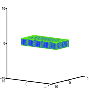
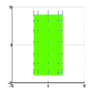
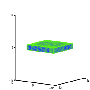
We present simulations of the dynamics of an LCE sample – using Equations (2.2.5–38) – when exposed to external illumination and subject to two different boundary conditions. The LCE sample is taken as box-shaped, as in Fig. 1a. In the first set of simulations, zero-stress boundary conditions are imposed over the sample surface (i.e., the sample is “free”). In the second case, one end of the sample is anchored to a wall, with the remainder free. In either case, gravitational loads are neglected. Numerically, the difference between these two cases lies only in the treatment of the velocity on one face of the sample. However, the dynamics the two cases present is quite different, as observed in [13].

3.1 Methods

To discretize the equations of motion, one needs to consider suitable schemes for approximating both spatial derivatives and time derivatives. here we employ the spectral Chebyshev polynomial method to discretize spatial derivatives with high efficiency and accuracy [15]. As for the time-discretization, we use a popular implicit-explicit scheme that is a combination of second-order Adams-Bashforth scheme for the explicit term and Crank-Nicolson scheme for the implicit term [1, 10, 15].

We now outline the Chebyshev polynomial method and the implicit-explicit time-stepping method. The dynamics is simulated in the Lagrangian domain $\Omega(0)=[-a,a]\times[-b,b]\times[-c,c]$, which by definition is fixed in time. This is trivially mapped to the cube $[-1,1]^{3}$. This cubic domain is then discretized in each direction on the Gauss-Lobatto points (e.g. in the first coordinate, $\mbox{{\boldmath$\alpha$}}_{1,j}=\cos(j\pi/N),~{}j=0(1)N$). This allows allows spatially dependent fields, such as $\mathbf{u}$ or $\mathbf{F}$, that are represented discretely on these points to also be represented efficiently, via FFT, as finite sums of Chebychev polynomials [15]. The Chebychev representation can then be used to provide highly accurate derivative approximations upon the grid. To illustrate in one dimension, let $u(x)$ be defined on $[-1,1]$ and approximated by $u_{N}(x)=\sum_{p=0}^{N}a_{p}T_{p}(x)$ where $T_{p}$ is the $p^{th}$ Chebychev polynomial. The $a_{p}$’s are determined by requiring $u_{N}$ to interpolate $u$ at the Gauss-Lobatto points. This Chebychev representation allows us to construct approximations to $u^{(p)}(x)$, at the Gauss-Lobatto points, that have the form

$$u_{N}^{(p)}(x_{i}) =\sum_{j=0}^{N}d^{(p)}_{ij}u_{N}(x_{j}),\hskip 14.22636pti=0(1)N,$$

where $[d^{(p)}_{ij}]$ is the the $p^{th}$ Chebyshev differentiation matrix (see [15]). Since our three-dimensional grid is of tensor product form, derivatives are easily gotten by application of such matrices along lines of constant coordinate of the discretized data.

The LCE dynamics in which we are interested takes place in the over-damped regime, that is the “Reynolds number”, $\lambda\gamma_{3}/\gamma_{1}$, associated with viscous fluid damping is very small. Hence, if we retain $\mathbf{u}_{t}$ in the dynamics, we must implicitly treat the viscous damping so as to avoid extreme constraints on the time-step that would be imposed by using an explicit scheme. Here, we choose a popular implicit-explicit method which is described for a typical time dependent equation:

$$\frac{du}{dt} =f(u)+\nu g(u),$$

with $f(\cdot)$, $g(\cdot)$ being nonlinear and linear terms, respectively. We apply a second-order Adams-Bashforth method to the nonlinear terms, and Crank-Nicholson averaging to the linear term, or

$$\frac{u^{n+1}-u^{n}}{\Delta t} =\frac{3}{2}f(u^{n})-\frac{1}{2}f(u^{n-1})+\frac{\nu}{2}[g(u^{n+1})+g(u^{n})],$$ (39)

where $\Delta t$ is the time step size and $u^{n}$ is the approximation of $u(n~{}\Delta t)$. This scheme involves solution values on three time levels. The first time-step is taken by setting $u^{-1}=u^{0}=u(0)$ (see [15]).

3.2 Treatment of interior and boundary points

Note that the equations (35) and (36) involve no spatial derivatives, and so are solved directly by the second-order Adams-Bashforth method and without using the Chebyshev approximation. More care must be taken with the momentum equation (2.2.5) as it is a source of stiffness in the numerical treatment, and since its advancement involves boundary conditions. This is an important issue, since distinct boundary conditions result in completely different behaviors of the LCE sample. In what follows, we mainly discuss how to handle the equation for both boundary and interior points.

The three-dimensional grid using the Gauss-Labatto points is composed of both surface and interior points. To update the velocity at the interior points, we need to solve a large linear system gotten by applying the implicit-explicit method for the velocity equation (2.2.5), coupling this to boundary conditions. For a “free” LCE sample, this is a condition of zero normal stress, which under discretization of velocity gradients in the viscous stress provides a coupling condition of the boundary velocities to the interior velocities.

The velocity equation (2.2.5) can be discretized as follows:

$$\frac{\mathbf{u}^{n+1}-\mathbf{u}^{n}}{\Delta t} =\frac{3}{2}\Bigl{[}\frac{1}{\lambda}\nabla\cdot(\Lambda(J-1)J\mathbf{F}^{-T}+\frac{1}{2}\mathbf{L}^{-1}\mathbf{F}\mathbf{L}_{0})\Bigr{]}^{n}$$

$$-\frac{1}{2}\Bigl{[}\frac{1}{\lambda}\nabla\cdot(\Lambda(J-1)J\mathbf{F}^{-T}+\frac{1}{2}\mathbf{L}^{-1}\mathbf{F}\mathbf{L}_{0})\Bigr{]}^{n-1}$$

$$+\frac{\gamma_{1}}{4\gamma_{3}}\nabla\cdot\Bigl{[}(\nabla\mathbf{u}^{n+1}(\mathbf{F}^{-1})^{n}+(\mathbf{F}^{-T})^{n}(\nabla\mathbf{u}^{T})^{n+1}(\mathbf{F}^{-T})^{n}\Bigr{]}$$

$$+\frac{\gamma_{1}}{4\gamma_{3}}\nabla\cdot\Bigl{[}(\nabla\mathbf{u}^{n}(\mathbf{F}^{-1})^{n-1}+(\mathbf{F}^{-T})^{n-1}(\nabla\mathbf{u}^{T})^{n}(\mathbf{F}^{-T})^{n-1}\Bigr{]},$$

where $[\cdot]^{n}$ represents the value at $\mbox{n}\Delta t$, for instance, $(\mathbf{F}^{-T})^{n}$ denotes the value of $\mathbf{F}^{-T}$ at $\mbox{n}\Delta t$. This equation amounts to a large linear system for the unknown velocity $\mathbf{u}^{n+1}$ at the interior points. Couplings within the matrix arise through expansion of spatial derivatives (that is, gradients and a tensor divergence) through the Chebyshev expansion of the velocity. Despite the many entries in the matrix generated through the derivatives, the matrix is nonetheless rather sparse, and we explicitly construct the entries and store this sparse matrix. Once the boundary conditions are appropriately integrated, we solve this large system using the iterative GMRES method [16].

Surface values of velocity are either additional unknowns, or are specified as in the case of having an anchored surface where $\mathbf{u}=0$ on that face. The former is the case of the zero stress boundary condition. In the Lagrangian frame, using Nanson’s formula [19], this boundary condition can be written as

$$\Bigl{[}\Lambda({J}-1)\mathbf{I}+\frac{1}{2}\mathbf{L}^{-1}\mathbf{F}\mathbf{L}_{0}\mathbf{F}^{T}\Bigr{]}\cdot{J}\mathbf{F}^{-T}\mathbf{\nu}_{0}+\frac{\gamma_{1}}{2\gamma_{3}}\Bigl{[}(\nabla_{\mbox{{\boldmath$\alpha$}}}\mathbf{u}\mathbf{F}^{-1}$$

$$+\mathbf{F}^{-T}\nabla_{\mbox{{\boldmath$\alpha$}}}\mathbf{u}^{T})\Bigr{]}\cdot{J}\mathbf{F}^{-T}\mathbf{\nu}_{0} =\mathbf{0},$$ (40)

where $\mathbf{\nu}_{0}$ denotes the outward normal unit vector to the time invariant surface $\partial\Omega(0)=\partial\Omega$. In our method, this vector $\nu_{0}$ takes different values at the side, edge and corner points on the boundary of the cubic volume of the LCE sample. Specifically, at the side points, $\nu_{0}$ takes value from the set $\{(\pm 1,0,0),(0,\pm 1,0),(0,0,\pm 1)\}$; at the edge points, the set becomes $\{\frac{1}{\sqrt{2}}(\pm 1,\pm 1,0)$, $\frac{1}{\sqrt{2}}(\pm 1,\mp 1,0)$, $\frac{1}{\sqrt{2}}(\pm 1,0,\pm 1)$,$\frac{1}{\sqrt{2}}(\pm 1,0,\mp 1)$, $\frac{1}{\sqrt{2}}(0,\pm 1,\pm 1)$, $\frac{1}{\sqrt{2}}(0,\pm 1,\mp 1)\}$; and at the corner points, the set is then $\{\frac{1}{\sqrt{3}}(\pm 1,\pm 1,\pm 1)$, $\frac{1}{\sqrt{3}}(\pm 1,\pm 1,\mp 1)$, $\frac{1}{\sqrt{3}}(\mp 1,\pm 1,\pm 1)$, $\frac{1}{\sqrt{3}}(\mp 1,\pm 1,\mp 1)\}$.

We rewrite the boundary condition equation (3.2) as:

$$\left[(\nabla_{\mbox{{\boldmath$\alpha$}}}\mathbf{u}\mathbf{F}^{-1}+\mathbf{F}^{-T}\nabla_{\mbox{{\boldmath$\alpha$}}}\mathbf{u}^{T})\right]\mathbf{F}^{-T}\mathbf{\nu}_{0} =\mathbf{A}\mathbf{\nu}_{0},$$

where $\mathbf{A}=-\frac{2\gamma_{3}}{\gamma_{1}}[\frac{1}{2}\mathbf{L}^{-1}\mathbf{F}\mathbf{L}_{0}+\Lambda(\mathbf{J}-1)J\mathbf{F}^{-T}]$. This boundary condition is evaluated at the $(n+1)$st time-step. Given that all of the dynamics equations, bar that for the velocity $\mathbf{u}$, are treated explicitly, we can consider $\mathbf{F}$ and $\mathbf{A}$ as being considered known, and the velocity gradients as unknowns. Gradients are either tangential to the sample surface, and hence only couple together boundary points (upon approximation of gradients using the Chebyshev representation), or normal to the surface and hence couple together boundary and interior points.

This yields a closed set of equations for $\mathbf{u}^{n+1}$ at the interior points, and on those surface upon which a zero stress boundary condition is imposed. As said above, this system is solved via the GMRES iterative method [16].

An important issue that should be emphasized is how to employ the GMRES method efficiently. Indeed, note that the coefficient matrix is very sparse, we just need to store the non-zero entries of the coefficient matrix, and also the row and column indices of these non-zero entries. Then in the matrix-vector multiplication, these non-zero entries will be multiplied by those elements of the vector using the above stored column indices. This procedure can save lots of memory and also accelerate the matrix-vector multiplication considerably.

3.3 Simulations

Before proceeding, we discuss the choice of dimesionless parameters. These include the coefficient of acceleration $\lambda=\rho_{c}kT\rho_{m}b^{2}/\gamma_{3}^{2}$, the viscosity ratio $\gamma_{1}/\gamma_{3}$, the coefficient for volume conservation $\Lambda$, and the anisotropy of step length $\mu$ appearing in the tensor $\mathbf{L}$. Taking typical values [13] we have $\lambda=O(10^{-3})$ and $\gamma_{1}/\gamma_{3}=O(10^{1-2})$. Hence, inertial forces in the material are quite small. Ideally, we should choose a very large value of $\Lambda$ to enforce material incompressibility, but this imposes a severe time-step restriction in our numerical scheme; We use $\Lambda=10^{3}$. The parameter $\mu$ lies in the range $[0,1.0]$. A large value of $\mu$ corresponds to a large order parameter, which accelerates the deformation process of the LCE sample. We use $\mu=0.9$ in the simulations.

We now consider the simulated dynamics of the first case of a “free” LCE sample being exposed to illumination from above. In this simulation, the sample size is $8\times 8\times 1$, with $N_{1}=32$, $N_{2}=32$ and $N_{3}=10$ points being used in each direction, respectively. The initial data used was $\mathbf{u}_{0}\equiv\mathbf{0}$, $\mathbf{n}_{0}\equiv\mathbf{{\hat{y}}}$, $\mathbf{X}_{0}\equiv\mathbf{\mbox{{\boldmath$\alpha$}}}$, and $s_{0}\equiv{\bar{s}}$, where ${\bar{s}}$ is the constant value found as the minimizer of the Landau-de Gennes free energy density (3) given a uniform temperature throughout the sample corresponding to 290K (in dimensional units). As discussed earlier, we neglect thermal diffusion and assume that the temperature is uniform in each horizontal slice of the sample, decreasing linearly from top (420K) to bottom (290K).

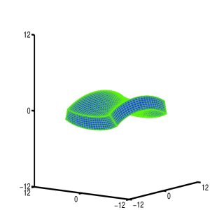
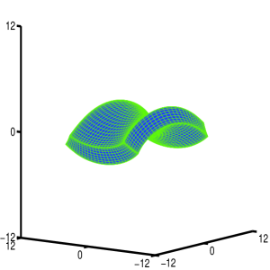
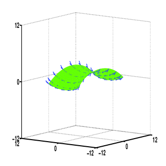
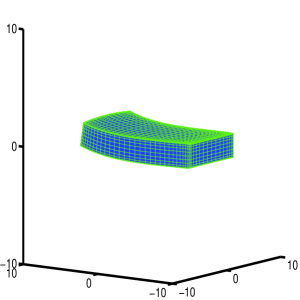
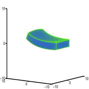
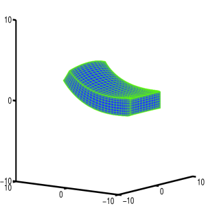
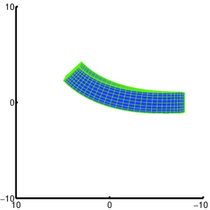
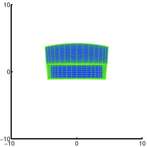
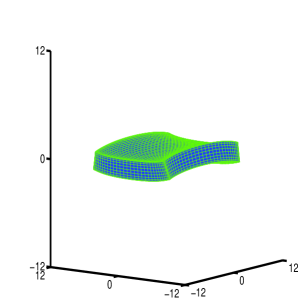
Figure 1 shows the deformation process from this initial configuration. The final result – a saddle shape – is very similar to that observed in the experiment of Palffy-Muhoray et al. (see Fig. 4 of [13]). The evolution proceeds in three stages: an initially slow and small bending, followed by rapid and large deformation, and finally a slow relaxation to a terminal shape. This dynamics is driven by the evolution of the orientational order parameter, $s$, as it adjusts its values (low on the top and higher on the bottom) in response to the imposed temperature gradient. The inhomogeneous spatial distribution of orientational order, especially through the thickness of the LCE sample, gives rise to large stresses and hence creates a strong driving force towards changing the shape of the sample.

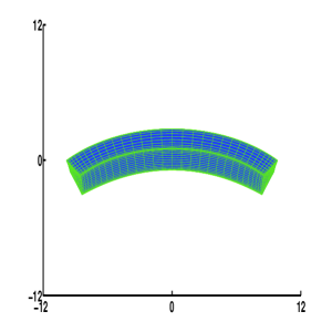
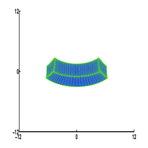
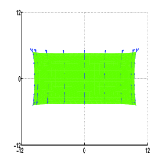
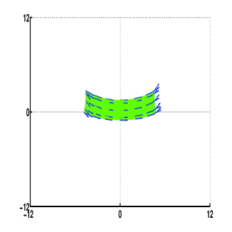
The last two plots of Fig. 1 show the late-time deformed sample from two different perspectives. Here one finds that the length along the $y-$axis has become shorter, while that along the $x-$axis has increased. This is again due to the time evolution of order parameter. At the top surface, given its increased temperature, the degree of order of the rod-like mesogens decreases. Since these mesogens are initially aligned along the $y-$direction, this loss of order leads to a contraction of the sample along the $y-$direction and corresponding extensions along the $x-$ and $z-$directions. Since the temperature is different on each horizontal layer, the degree of contraction also is also different. It is this difference in contraction and expansion through the thickness of LCE sample that results in the observed saddle-shaped deformation.

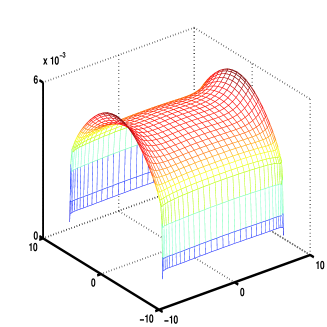
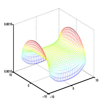
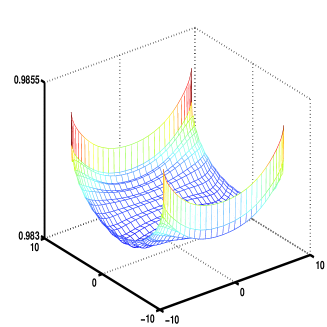
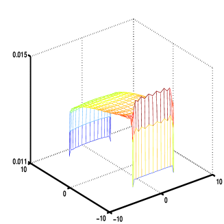
The simulation shows that as the dynamics progresses, the order parameter in each horizontal layer converges to nearly constant values essentially determined by the temperature assigned to that layer (see Eq. (35)), though somewhat affected also by elastic effects induced by coupling to $\mathbf{n}$. This is illustrated in Figure 2, which shows that the order parameter generally assume smaller values at the top and larger values on the bottom, but also varies (slightly) within each layer.

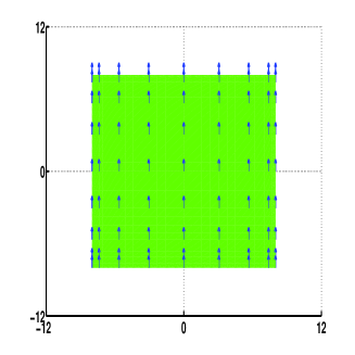
We also study the dynamics of nematic director $\mathbf{n}$. In Figure 3, the nematic director on the top surface of the sample is compared at the initial and equilibrium states. For the equilibrium state, three perspectives are given from which one can easily discern the evolution of the nematic director. Similar director distributions on the other layers of the sample can be observed.

The dynamics of the second simulation can be explored similarly. In this simulation, all initial conditions and spatial temperature distributions are as in the first example, except that one lateral surface of the sample is fixed, and the dimensions of the LCE sample are now $4\times 8\times 1$, which is narrower in the $x-$direction.

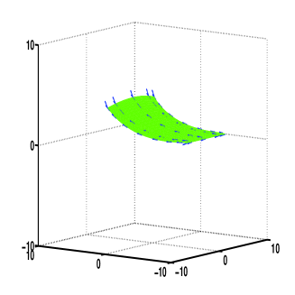
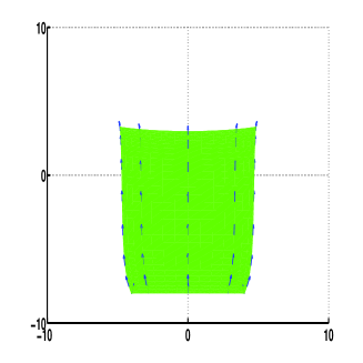
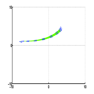
Figure 4 shows the deformation process. Again, the result is very similar to that observed in actual experiment (see Fig. 2 of [13]) with the sample bending upwards at its free end. As the in first simulation, the deformation proceeds through three stages, with the sample also contracting along the initial nematic direction and extending in the other two orthogonal directions. This is illustrated the Figs. 4E and F. All these phenomena share the underlying physics as in the first simulation.

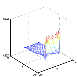
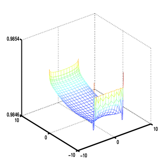
In Figure 5, the order parameter distributions within the top, middle, and bottom layers of the sample in the equilibrium state are shown. The order parameter within each layer is nearly constant within each layer, though with small oscillations caused by boundary effects. However, when compared with Fig. 2 for the first simulation, one finds that the basic deformation pattern is different and asymmetric due to the anchoring boundary condition used in this experiment.

Figure 6, shows the disposition of the nematic director on the top surface of the LCEs sample, again comparing the initial and the equilibrium states. For the equilibrium state, three perspectives are shown. We see that the nematic director bends upwards, and the bending increases with distance from the fixed side of the sample. Similar director dynamics are observed in the other layers.

($\mathbf{A}$)                                             ($\mathbf{B}$)

($\mathbf{C}$)                                             ($\mathbf{D}$)

($\mathbf{E}$)                                             ($\mathbf{F}$)

Figure 1: The shape evolution of the LCEs sample due to nonhomogeneous changes in temperature. Figure $\mathbf{A}$ shows the initial state of the LCEs sample, while Figures $\mathbf{B}$, $\mathbf{C}$ are two intermediate states and Figure $\mathbf{D}$ represents the equilibrium state. Figures $\mathbf{E}$ and $\mathbf{F}$ present the shape of the LCEs sample at the equilibrium state (Figure $\mathbf{D}$) from two different perspectives. In this experiment, the temperature drops linearly from the top of the LCEs sample to its bottom while distributes uniformly on each horizontal slices, and the temperature spatial distribution is preserved during the evolution process. This numerical experiment simulates the real one shown in Figure 4 in [13].

($\mathbf{A}$)                                             ($\mathbf{B}$)

$\mathbf{C}$

Figure 2: The order parameter (S) distribution for the top ($\mathbf{A}$), middle ($\mathbf{B}$) and bottom ($\mathbf{C}$) horizontal slices of the LCEs sample at the equilibrium state. The order parameter is close to zero on the top slice while it is close to one on the bottom slice. It is the nonhomogeneous distribution of the order parameter that leads to internal stress, and thus results in the shape changes of the LCEs sample. Moreover, the order parameter slightly varies on each of these slices, suggesting the elastic effect on the order parameter.

($\mathbf{A}$)

($\mathbf{B}$)                                             ($\mathbf{C}$)

($\mathbf{D}$)

Figure 3: The nematic direction ($\mathbf{n}$) distribution for the top slice of the LCEs sample at the initial and the equilibrium state. The plot ($\mathbf{A}$) represents the nematic direction on the top slice at the initial state. The plots ($\mathbf{B}$), ($\mathbf{C}$) and ($\mathbf{D}$) illustrate the nematic direction on the top slice for different perspectives at the equilibrium state.

($\mathbf{A}$)                                             ($\mathbf{B}$)

($\mathbf{C}$)                                             ($\mathbf{D}$)

($\mathbf{E}$)                                             ($\mathbf{F}$)

Figure 4: The shape evolution of the LCEs sample due to nonhomogeneous changes in temperature. Figure $\mathbf{A}$ shows the initial state of the LCEs sample, while Figures $\mathbf{B}$, $\mathbf{C}$ are two intermediate states and Figure $\mathbf{D}$ represents the equilibrium state. Figures $\mathbf{E}$ and $\mathbf{F}$ present the shape of the LCEs sample at the equilibrium state (Figure $\mathbf{D}$) from two different perspectives. This experiment shares the same condition as the previous simulation in Figure 1 except that a lateral surface of the LCEs sample is fixed. This numerical experiment simulates the real one shown in Figure 2 in [13].

($\mathbf{A}$)                                             ($\mathbf{B}$)

$\mathbf{C}$

Figure 5: The order parameter (S) distribution for the top ($\mathbf{A}$), middle ($\mathbf{B}$) and bottom ($\mathbf{C}$) horizontal slices of the LCEs sample at the equilibrium state. The order parameter is close to zero on the top slice while it is close to one on the bottom slice. It is the nonhomogeneous distribution of the order parameter that leads to internal stress, and thus results in the shape changes of the LCEs sample. Moreover, the order parameter slightly varies on each of these slices and oscillates near the fixed lateral surface of the LCEs sample, suggesting both the elastic effect and the effect due to the anchored surface on the order parameter.

($\mathbf{A}$)

($\mathbf{B}$)                                             ($\mathbf{C}$)

($\mathbf{D}$)

Figure 6: The nematic direction ($\mathbf{n}$) distribution for the top slice of the LCEs sample at the initial and the equilibrium state. The plot ($\mathbf{A}$) represents the nematic direction on the top slice at the initial state. The plots ($\mathbf{B}$), ($\mathbf{C}$) and ($\mathbf{D}$) illustrate the nematic direction on the top slice for different perspectives at the equilibrium state.

4 Conclusions

In this paper, we derived the equations of motion for an LCE sample in the long-wave limit, and implemented their numerical solution. Our numerical experiments demonstrate that the model is capable of describing the dynamics of nematic LCEs when exposed to external stimuli such as illumination.

5 Acknowledgements

The authors acknowledge the support of the NSF and DOE.

References

• [1] U.R. Acher, S.J. Ruuth, and B.T.R. Wetton, Implicit-explicit methods for time-dependent partial differential equations, SIAM J. Numer. Anal. 32 (3), pp. 797-823, 1995.
• [2] H.R. Brand and H. Pleiner, Electrohydrodynamics of nematic liquid crystalline elastomers, Physica A 208, pp 359-359, 1994.
• [3] J. Cviklinski, A.R. Tajbakhsh, and E.M. Terentjev, UV is isomerisation in nematic elastomers as a rounte to photo-mechanical transducer, Eur. Phys. J. E. 9, pp. 427-434, 2002.
• [4] S.M. Clarker, A.R. Tajbakhsh, E.M. Terentjev, and M. Warner, Anomalous viscoelastic response of nematic elastomers, Phys. Rev. Lett. 86, pp. 4044-4047, 2001.
• [5] P. G. de Gennes, Re´´𝑒\acute{e}flexions sur un type de polymeres ne´´𝑒\acute{e}matiques, C. R. Acad. Sci., Ser. B 281, pp. 101-103, 1975.
• [6] P. G. de Gennes and J. Prost, The Physics of Liquid Crystals, Oxford University Press, Oxford, 1993.
• [7] R. Ennis, L.C. Malacarne, P. Palffy-Muhoray, and M. Shelley, Nonlocal model for nematic liquid-crystal elastomers, Physical Review E 74, 061802, 2006.
• [8] H. Finkelmann, H. Kock, and G. Rehage, Makromol, Investigation on LC polysiloxanes: 3. Liquid crystalline elastomers — a new type of liquid crystalline material, Makromol. Chem. Rapid Commun. 2, pp. 317-317, 1981.
• [9] H. Finkelmann, E. Nishikawa, G.G. Pereira, M. Warner, A New opto-mechanical effect in solids, Phys. Rev. Lett. 87, 015501, 2001.
• [10] B. Gustafsson, H.O. Kreiss, and J. Oliger, Time dependent problems and difference methods, John Wiley and Sons, INC, 1995.
• [11] G. Holzapfel, Nonlinear Solid Mechanics, Wiley, Chichester, 2000.
• [12] C. Oldano and G. Barbero, An AB initio analysis of the second-order elasticity effect on nematic configurations, Phy. Lett. A, 110 (4) pp. 213-216, 1985.
• [13] P. Palffy-Muhoray, M. Camancho-Lopez., H. Finkelmann, and M. Shelley, Fast Liquid Crystal Elastomer Swins Into the Dark, Nat. Mat. 3, 307-310, 2004.
• [14] P. Palffy-Muhoray, W. Cao, M. Moreira, B. Taheri and A. Munoz, Photonics and lasing in liquid crystal materials, Phil. Trans. R. Soc. A 364, pp. 2747 2761, 2006
• [15] R. Peyret, Spectral methods for incompressible viscous flow, Springer-Verlag New York, Inc., 2002.
• [16] Y. Saad and M.H. Schultz, GMRES: A generalized minimal residual algorithm for solving nonsymmetric linear systems, SIAM J. Sci. Comput. Vol 7(3), pp. 856-869, 1986.
• [17] E.M. Terentjev, S. Hotta, M. Clarke, and M. Warner, Liquid crystalline elastomers: dynamics and relaxation of microstructure, Phil. Trans. R. Soc. Lond. A, 361, pp. 1-12, 2003.
• [18] M. Warner and E. M. Teretjev, Liquid Crystal Elastomers, Clarendon Press, Oxford, 2003.
• [19] G. Holzapfel, Nonlinear Solid Mechanics, Wiley, Chichester, 2000.
• [20] Y. Yu, M. Nakano, and T. Ikeda, Directed bending of a polymer film by light, Nature 425, pp. 145-145, 2003.
• [21] T.J. White, J.J. Koval, V.P. Tondiglia, L.V. Natarajan, R.A. Vaia, S. Serak, V. Grozhik, N. Tabirian, and T.J. Bunning, Polarization dependent photoactuation in azobenzene LC polymers, Proc. SPIE 6654, 665403/665401 665403/665405, 2007.