The electroweak fit and constraints on new physics

The global electroweak fit of the Standard Model (SM) with Gfitter can be used to constrain yet unknown SM parameters, such as the Higgs mass, but also physics beyond the SM (BSM) via the formalism of oblique parameters. This paper presents updated results of the Gfitter SM fit using the latest available electroweak precision measurements and the recent combination of direct Higgs searches at the Tevatron. In addition, newly obtained constraints on BSM models, such as models with extra dimensions, little Higgs and a fourth fermion generation, are presented. While a light Higgs mass is preferred by the fit in the SM, significantly larger Higgs masses are allowed in these new physics models.

1 Introduction

By exploiting contributions from radiative corrections precise measurements can be used to obtain insights into physics at much higher energy scales than the masses of the particles directly involved in the experimental reactions. In combination with accurate theoretical prediction the experimental data allow us to constrain the free parameters of the physics model in question. Using this principle, in particular the yet unknown mass of the Higgs boson $M_{H}$, can be constrained in the Standard Model (SM) using the electroweak precision measurements and state-of-the-art SM predictions since $M_{H}$ enters logarithmically the prediction of higher-order corrections in the SM. Furthermore, in models describing physics beyond the SM (BSM) new effects, e.g. from additional heavy particles entering the loops, can influence the prediction of the radiative corrections of the electroweak observables. The formalism of oblique parameters, which parametrize the new physics contribution to the radiative corrections, can then be used to probe the new physics models and constrain their free parameters.

In this paper we present updated results of the global electroweak fit with the Gfitter framework $\!{}^{{\bf?}}$ taking into account the latest experimental precision measurements and the results of direct Higgs searches from LEP and Tevatron. In addition, we present newly obtained constraints on BSM models with extra dimensions, little Higgs and a fourth fermion generation using the oblique parameters.

2 The global electroweak fit of the SM with Gfitter

A detailed discussion of the statistical methods, the experimental data, the theoretical calculations and the results of the global electroweak fit with Gfitter can be found in our reference paper $\!{}^{{\bf?}}$. Since its publication the fit has been continuously maintained and kept in line with experimental and theoretical progress. In the following the most important aspects of the fit are quickly repeated and results of recent changes – mainly updates of the experimental data used in the fit, e.g. $M_{W}$, $m_{t}$ and the direct Higgs searches at the Tevatron – are reported.

The SM predictions for the electroweak precision observables measured by the LEP, SLC, and Tevatron experiments are fully implemented in Gfitter. State-of-the-art calculations have been used, in particular the full two-loop and the leading beyond-two-loop corrections for the prediction of the $W$ mass and the effective weak mixing angle $\!{}^{{\bf?}}$, which exhibit the strongest constraints on the Higgs mass. In the Gfitter SM library the fourth-order (3NLO) perturbative calculation of the massless QCD Adler function $\!{}^{{\bf?}}$ is included which allows to fit the strong coupling constant with unique theoretical uncertainty.

Figure 1: (left) $\Delta\chi^{2}$ profile as a function of $M_{H}$ for the global fit of the electroweak SM with Gfitter including the results of the direct Higgs searches at LEP and Tevatron. The regions currently excluded with 95 % CL by LEP and Tevatron are indicated by the shaded areas. (right) Fit result of the oblique parameters: Shown are the 68 %, 95 % and 99 % CL allowed regions in the $(S,T)$-plane with $U=0$ for a reference SM with $M_{H}=120$ GeV and $m_{t}=173.2$ GeV. The gray/dark area illustrates the SM prediction for various values of $M_{H}$ and $m_{t}$.

The experimental data used in the fit include the electroweak precision data measured at the $Z$ pole $\!{}^{{\bf?}}$, the latest world average $\!{}^{{\bf?}}$ of the $W$ mass $M_{W}=(80.399\pm 0.023)$ GeV, and width $\Gamma_{W}=(2.098\pm 0.048)$ GeV, which include the recent run-2 mass measurement reported by D0, and the newest average $\!{}^{{\bf?}}$ of the Tevatron top mass measurements $m_{t}=(173.1\pm 1.3)$ GeV. For the electromagnetic coupling strength at $M_{Z}$ we use the $\Delta\alpha^{(5)}_{\rm had}$ value reported in  $\!{}^{{\bf?}}$ which does not include the recent ISR measurements of the $e^{+}e^{-}\to\pi^{+}\pi^{-}$ cross-section from Babar and Kloe since an updated $\Delta\alpha^{(5)}_{\rm had}$ value including both measurements is not yet available. Also included in the fit is the information from the direct Higgs searches at LEP $\!{}^{{\bf?}}$ and Tevatron $\!{}^{{\bf?}}$, where we use the latest combination.

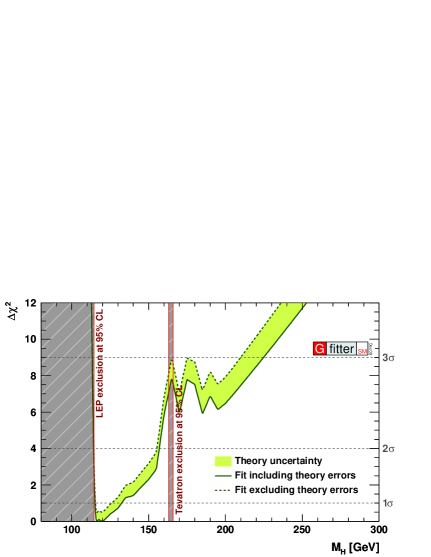
The free fit parameters are $M_{Z}$, $M_{H}$, $m_{t}$, $m_{b}$, $m_{c}$, $\Delta\alpha^{(5)}_{\rm had}$ and $\alpha_{S}(M_{Z}^{2})$ where only the latter parameter is fully unconstrained since no direct experimental measurement of $\alpha_{S}(M_{Z}^{2})$ is used. The minimum $\chi^{2}$ value of the fit with (without) using the information from the direct Higgs searches amounts to 17.8 (16.4) which corresponds to a $p$-value for wrongly rejecting the SM of 0.22 (0.23). None of the pull values exceeds 3$\sigma$. The 3NLO result of $\alpha_{S}(M_{Z}^{2})$ obtained from the fit is given by $\alpha_{S}(M_{Z}^{2})=0.1193\pm 0.0028\pm 0.0001$, where the first error is the experimental fit error and the second is due to missing QCD orders. Among the most important outcomes of the fit is the estimation of the mass of the Higgs boson. Without using the information from the direct Higgs searches we obtain a $\chi^{2}$ minimum at $M_{H}=82.8^{+30.2}_{-23.3}$ GeV with a 2$\sigma$ interval of $[41,158]$ GeV. The combination of the indirect fit with the direct Higgs searches can be used to significantly reduce the allowed regions for $M_{H}$ in the SM. The resulting $\Delta\chi^{2}$ profile as a function of $M_{H}$ is shown in Fig. 1 (left). The expected strong increase at the LEP 95% CL exclusion limit and the contribution of the Tevatron searches at higher masses are clearly visible. We obtain a $\chi^{2}$ minimum at $M_{H}=119.4^{+13.4}_{-4.0}$ GeV with a 2$\sigma$ interval of $[114,157]$ GeV.

3 Constraints on new physics models

A common approach to constrain physics beyond the SM using the global electroweak fit is the formalism of oblique parameters. Assuming that the contribution of new physics models only appears through vacuum polarization most of the BSM effects on the electroweak precision observables can be parametrized by three gauge boson self-energy parameters ($S$, $T$, $U$) introduced by Peskin and Takeuchi $\!{}^{{\bf?}}$. In this approach the prediction of a certain electroweak observable $O$ is given by the sum of the prediction of a reference SM ($\rm SM_{ref}$, defined by fixing the values for $M_{H}$ and $m_{t}$) and the new physics effects parametrized by $STU$, i.e. $O=O_{\rm SM,ref}(M_{H},m_{t})+c_{S}S+c_{T}T+c_{U}U$. The parameters $STU$ hence measure deviations of the data from the chosen $\rm SM_{ref}$. They vanish if the data are equal to the $\rm SM_{\rm ref}$ prediction. $S$ ($S+U$) is sensitive to BSM contributions to neutral (charged) current processes at different energy scales, while $T$ is sensitive to isospin violation effects. The parameter $U$ is small in most BSM models. Further generalizations like additional corrections to the $Zbb$ coupling $\!{}^{{\bf?}}$ are also taken into account in Gfitter.

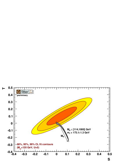
Following this approach we have determined the oblique parameters from the electroweak fit. For a $\rm SM_{\rm ref}$ with $M_{H}=120$ GeV and $m_{t}=173.2$ GeV we obtain

$$S=0.02\pm 0.11,\quad\quad\quad T=0.05\pm 0.12;\quad\quad\quad U=0.07\pm 0.12\quad.$$ (1)

The correlation between $S$ and $T$ is strong and positive ($+0.879$) while the correlation between $S$ and $U$ and between $T$ and $U$ is negative ($-0.469$ and $-0.716$, respectively). Figure 1 (right) shows the 68%, 95% and 99% CL allowed contours in the $(S,T)$-plane for $U=0$, together with the SM prediction featuring a logarithmic dependence on $M_{H}$. Apart from the trivial fact that the prediction for our $\rm SM_{ref}$ ($M_{H}=120$ GeV, $m_{t}=173.2$ GeV) is indeed $S=T=U=0$, it can be seen that the data are compatible with the SM prediction for small values of $M_{H}$. Hence, no actual need for new physics can be derived from this study.

However, certain BSM models feature a similar agreement with the data. The prediction of these models can cover large regions in the $ST$-plane due to the allowed variation of the additional free model parameters which in turn can be constrained by comparing the experimental data and the model prediction. As shown in the following, in some BSM models large values of $M_{H}$ are allowed due to a possible compensation of BSM and Higgs effects.

3.1 Universal Extra Dimensions

Figure 2: Example results for a model with one Universal Extra Dimension: (left) Comparison of the $STU$-fit result with the prediction in the UED model for various values of the compactification scale $R^{-1}$ and the Higgs mass $M_{H}$. (right) The 68 %, 95 % and 99 % CL allowed regions in the $(M_{H},R^{-1})$-plane as derived from the fit.

As a first example we discuss a model with additional space dimensions accessible for all SM particles $\!{}^{{\bf?}}$ (UED). In these models the conservation of a Kaluza-Klein (KK) parity leads to a phenomenology similar to supersymmetry with a stable lightest KK state, which is a candidate particle for the cold dark matter in the universe. The free parameters of the model are the number of extra dimensions $d_{ED}$ and the compactification scale $R^{-1}$. The contribution to the electroweak precision observables via vacuum polarisation effects in these models, i.e. the prediction of the $STU$ parameters, have been calculated in $\!{}^{{\bf?}}$. The main contribution results from additional KK-top/bottom and KK-Higgs loops. For $d_{ED}=1$, as assumed in the following, the prediction of the oblique parameters mainly depends on $R^{-1}$ and $M_{H}$.

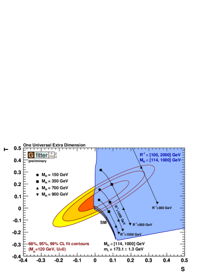
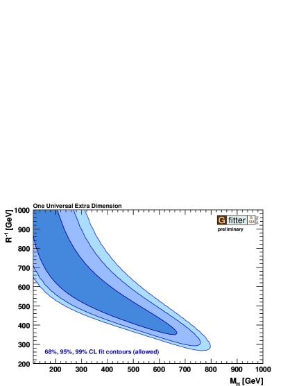
In Fig. 2 (left) the experimental fit result in the $(S,T)$-plane is compared to the UED prediction for various values of $R^{-1}$ and $M_{H}$. It can be seen that for high values of $R^{-1}$ the UED prediction approaches the SM expectation while for smaller $R^{-1}$ values a significant deviation from the SM prediction is expected. The same behavior can be observed in Fig. 2 (right) where the resulting 68%, 95% and 99% CL allowed regions in the $(M_{H},R^{-1})$-plane are shown. For high $R^{-1}$ values the constraint on $M_{H}$ approaches the SM result, i.e. small $M_{H}$ are preferred, while for small $R^{-1}$ values, significantly larger $M_{H}$ values are still allowed since the UED contribution is compensated by a heavier Higgs boson. The latter parameter region is well within the direct discovery reach of the LHC since $R^{-1}$ indicates the expected mass region of the additional KK states. The region $R^{-1}<300$ GeV and $M_{H}>750$ GeV can be excluded at 95% CL. These findings are in agreement with previous publications $\!{}^{{\bf?}}$.

3.2 Littlest Higgs model with T-parity conservation

Little Higgs theories tackle the SM hierarchy problem by introducing a new global symmetry broken at a scale $f\sim 1$ TeV where new SM-like fermions and bosons exist canceling the one-loop quadratic divergengies of $M_{H}$ in the SM. The Littlest Higgs (LH) Model $\!{}^{{\bf?}}$ is based on a non-linear 1$\sigma$ model describing an SU(5)/SO(5) symmetry breaking. Similar to $R$-parity conservation in supersymmetry, $T$-parity conservation provides a possible cold dark matter candidate and, important for the current discussion, it forbids tree-level contribution from heavy gauge bosons to the electroweak observables. In this case the dominant oblique corrections $\!{}^{{\bf?}}$ rather result from loops involving the two new heavy top states ($T$-even and $T$-odd). The corrections depend on the scale $f$, the ratio of the top state masses $s_{\lambda}=m_{T^{-}}/m_{T^{+}}$, $M_{H}$ and a coefficient $\delta_{c}$ whose exact value depends on details of the UV physics.

Figure 3: Example results for the Littlest Higgs model with $T$-parity conservation: (left) Comparison of the $STU$-fit result with the prediction in the LH model. The symbols illustrate the LH predictions for three example settings of the parameters $f$, $s_{\lambda}$ and $M_{H}$. The light green area illustrates the predicted region when varying the free parameters in the ranges indicated in the figure. (right) The allowed region in the $(M_{H},f)$-plane as derived from the fit for $s_{\lambda}=0.45$.

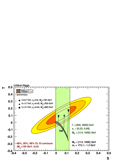
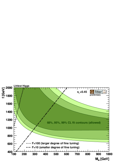
In Fig. 3 (left) the experimental fit result in the $(S,T)$-plane is compared to the LH prediction for example values of $f$, $s_{\lambda}$ and $M_{H}$. It can be seen that for certain parameter settings the LH model with $T$-conservation is indeed in agreement with the data. In Fig. 3 (right) the fit results for $s_{\lambda}=0.45$ are illustrated as 68%, 95% and 99% CL allowed regions in the $(M_{H},f)$-plane. As expected, for high values of $f$ the $M_{H}$-constraint in the LH model approaches the $M_{H}$-constraint of the SM, while for smaller $f$ values significantly larger values of $M_{H}$ are allowed than in the SM. Although the allowed regions in the $(M_{H},f)$-plane are strongly dependent on $s_{\lambda}$ and no absolute exclusion limit on one of the parameters alone can be derived, the above statements are true for all values of $s_{\lambda}$.

3.3 Models with a fourth fermion generation

While the fermion sector of the Standard Model is composed of three generations of leptons and quarks without explanation of this number, several SM extensions suggest extra matter families. In a simple, generic model with only one extra family two new fermions $(\Psi_{1},\Psi_{2})$ are added to both the quark and lepton sector, i.e. a left-handed isospin doublet $\Psi_{L}=(\Psi_{1},\Psi_{2})_{L}$ and two right-handed isospin singlet states $\Psi_{1,R}$ and $\Psi_{2,R}$ with charges equal to the three SM generations. The free model parameters are the masses of the new quarks and leptons $m_{u_{4}}$, $m_{d_{4}}$, $m_{e_{4}}$ and $m_{\nu_{4}}$ respectively. Assuming no mixing of the extra families among themselves and with the SM fermions the additional one-loop fermionic contributions to the oblique corrections have been calculated in $\!{}^{{\bf?}}$. In particular, the importance of an appropriate mass splitting of the up-type and down-type fermions has been highlighted.

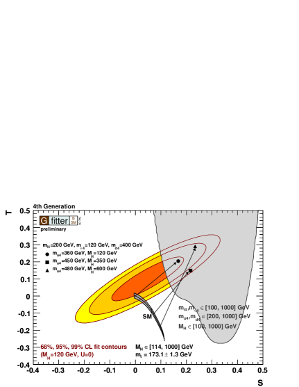
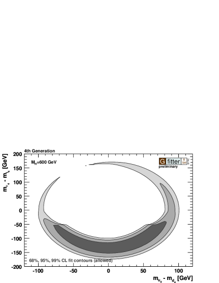
In Fig. 4 (left) our experimental fit result in the $(S,T)$-plane is compared to the prediction of the fourth generation model for example values of the masses of the additional fermions and $M_{H}$. It can be seen that for some parameter settings the fourth generation model is indeed in agreement with the data and high values of $M_{H}$ could in principle be allowed. Since the oblique parameters are mainly sensitive to the mass differences of the up-type and down-type fermions and rather insensitive to the absolute mass values of the additional fermions, we have calculated the 68%, 95% and 99% CL allowed regions in the $(m_{u_{4}}-m_{d_{4}},m_{l_{4}}-m_{{\nu}_{4}})$-plane for various values of $M_{H}$. The example results for $M_{H}=600$ GeV, shown in Fig. 4 (right), demonstrate that a high Higgs mass is indeed in agreement with the data for a range of new fermion masses. In general, the data prefer a heavier charged lepton.

Figure 4: Example results for a model with a fourth fermion generation: (left) Comparison of the $STU$-fit result with the prediction in the fourth generation model. The symbols illustrate the predictions for three example settings of the parameters $m_{U_{4}}$, $m_{d_{4}}$, $m_{{\nu}_{4}}$, $m_{l_{4}}$ and $M_{H}$. The light gray area illustrates the predicted region when varying the free parameters in the ranges indicated in the figure. (right) The allowed regions in the $(m_{u_{4}}-m_{d_{4}},m_{l_{4}}-m_{{\nu}_{4}})$-plane as derived from the fit for $M_{H}=600$ GeV.

4 Conclusion and outlook

Using the Gfitter package, the reimplementation of the global fit to the electroweak precision data and its combination with the recent results of the direct Higgs searches allows an exclusion of the SM Higgs mass above 158 GeV at 95% CL. However, contributions from new physics may change this result significantly. The effects on the gauge boson self-energy graphs, called oblique corrections, are known for most of the BSM models and must be continuously confronted with the latest experimental data. Newly obtained results of a few example BSM models implemented in Gfitter have been reported in this paper, demonstrating that larger $M_{H}$ values are in agreement with the electroweak precision data in these models. Apart from an continuous maintenance of the results reported here, an important future objective of Gfitter will be a further diversification of the latter analysis towards more BSM models.

References

- [1] H. Flächer et al., Eur. Phys. J. C 60, 543 (2009), [arXiv:0811.0009], updates and newly obtained results available at www.cern.ch/gfitter.
- [2] M. Awramik et al., Phys. Rev. D 69, 053006 (2004); M. Awramik et al., JHEP 11, 048 (2006).
- [3] P. A. Baikov et al., Phys. Rev. Lett. 101, 012022 (2008).
- [4] ADLO + SLD collaborations, Phys. Rept. 427, 257 (2006).
- [5] ADLO collaborations, [hep-ex/0612034]; CDF collabroation, Phys. Rev. D 77, 112001 (2008); D0 collabroation, Phys. Rev. Lett. 103, 141801 (2009); D0 collaboration, Phys. Rev. Lett. 103, 141801 (2009); Tevatron Elektroweak Working Group, [arXiv:0808.0147]; Tevatron Elektroweak Working Group, [arXiv:0908.1374].
- [6] Tevatron Elektroweak Working Group, [arXiv:0903.2503].
- [7] K. Hagiwara et al., Phys. Lett. B 649, 173 (2007).
- [8] ADLO collaborations, Phys. Lett. B 565, 61 (2003).
- [9] Tevatron New Physics Higgs Working Group, [arXiv:0911.3930].
- [10] M. E. Peskin and T. Takeuchi, Phys. Rev. D 46, 381 (1991).
- [11] C. P. Burgess et al., Phys. Lett. B 326, 276 (1994); C. P. Burgess et al., Phys. Rev. D 49, 6115 (1994).
- [12] T. Appelquist et al., Phys. Rev. D 67, 055002 (2003); I. Gogoladze et al., Phys. Rev. D 74, 093012 (2006).
- [13] N. Arkani-Hamed et al., JHEP 0207:034 (2002).
- [14] J. Hubisz et al., JHEP 0601:135 (2006).
- [15] H. He et al., Phys. Rev. D 64, 053004 (2001).