Evidence for power-law Griffiths singularities in a layered Heisenberg magnet
Abstract
We study the ferromagnetic phase transition in a randomly layered Heisenberg model. A recent strong-disorder renormalization group approach [Phys. Rev. B 81, 144407 (2010)] predicted that the critical point in this system is of exotic infinite-randomness type and is accompanied by strong power-law Griffiths singularities. Here, we report results of Monte-Carlo simulations that provide numerical evidence in support of these predictions. Specifically, we investigate the finite-size scaling behavior of the magnetic susceptibility which is characterized by a non-universal power-law divergence in the Griffiths phase. In addition, we calculate the time autocorrelation function of the spins. It features a very slow decay in the Griffiths phase, following a non-universal power law in time.
1 Introduction
Impurities, defects, and other types of quenched disorder influence zero-temperature quantum phase transitions much more strongly than generic classical phase transitions that occur at nonzero temperatures. The interplay of quantum and disorder fluctuations produces unconventional phenomena such as power-law quantum Griffiths singularities [1, 2, 3], infinite-randomness critical points featuring exponential instead of power-law scaling [4, 5], and smeared phase transitions [6, 7]. A recent review of these phenomena can be found in Ref. [8], while Ref. [9] focuses on metallic systems and also discusses experiments.
Disorder effects are stronger at quantum phase transitions than at classical transitions because the quenched disorder is perfectly correlated in the imaginary time direction. Imaginary time acts as an extra dimension at a quantum phase transition and becomes infinitely extended at zero temperature. Therefore, the impurities and defects are effectively “infinitely large” in this extra dimension, which makes them much harder to average out than finite-size defects.
This argument suggests that strong disorder effects should also occur at a classical thermal phase transition provided that the disorder is perfectly correlated in one or more space dimensions. An example occurs in the McCoy-Wu model, a disordered classical two-dimensional Ising model having perfect disorder correlations in one of the two dimensions. McCoy and Wu [10, 11, 12, 13] showed that this model exhibits an unusual phase transition featuring a smooth specific heat while the susceptibility is infinite over an entire temperature range. Fisher [4, 5] achieved an essentially complete understanding of this phase transition with the help of a strong-disorder renormalization group approach (using the equivalence between the McCoy-Wu model and the random transverse-field Ising chain). He determined that the critical point is of exotic infinite-randomness type and is accompanied by power-law Griffiths singularities.
Recently, some of us investigated another classical system with perfectly correlated disorder, the randomly layered Heisenberg magnet, by means of a strong-disorder renormalization group [14]. This theory predicts that the (thermal) critical point in the randomly layered Heisenberg magnet is of infinite-randomness type as well. Moreover, it is in the same universality class as the quantum critical point of the random transverse-field Ising chain. In this paper, we present the results of Monte-Carlo simulations of the randomly layered Heisenberg model. They provide numerical evidence in support of the above renormalization group predictions.
2 Model and renormalization group predictions
We consider a ferromagnet consisting of a random sequence of layers made up of two different ferromagnetic materials. Its Hamiltonian, a classical Heisenberg model on a three-dimensional lattice of perpendicular size (in direction) and in-plane size (in the and directions) is given by
| (1) |
Here, is a three-component unit vector on lattice site , and , , and are the unit vectors in the coordinate directions. The interactions within the layers, , and between the layers, , are both positive and independent random functions of the perpendicular coordinate . In the following, we take all to be identical, , while the are drawn from a binary probability distribution with . Here, is the concentration of the “weak” layers.
The qualitative behavior of (1) is easily explained. At sufficiently high temperatures, the model is in a conventional paramagnetic phase. Below a temperature (the transition temperature of a hypothetical system having for all ) but above the actual critical temperature , rare thick slabs of strong layers develop local order while the bulk system is still nonmagnetic. This is the paramagnetic Griffiths phase (or Griffiths region). In the ferromagnetic Griffiths phase, located between and a temperature (the transition temperature of a hypothetical system having for all ), bulk magnetism coexists with rare nonmagnetic slabs. Finally, below , the system is in a conventional ferromagnetic phase.
In Ref. [14], the behavior in both Griffiths phases and at criticality has been derived within a strong-disorder renormalization group calculation. Here, we simply motivate and summarize the results. The probability of finding a slab of consecutive strong layers is given by simple combinatorics; it reads with . Each such slab is equivalent to a two-dimensional Heisenberg model with an effective interaction . Because the two-dimensional Heisenberg model is exactly at its lower critical dimension, the renormalized distance from criticality, , of such a slab decreases exponentially with its thickness, [8, 15]. Combining the two exponentials gives a power law spectrum of locally ordered slabs,
| (2) |
where the second equality defines the conventionally used dynamical exponent, . It increases with decreasing temperature throughout the Griffiths phase and diverges as at the actual critical point.
Many important observables follow from appropriate integrals of (2). The susceptibility can be estimated by . In an infinite system, the lower bound of the integral is 0; therefore, the susceptibility diverges in the entire temperature region where . A finite system size in the in-plane directions introduces a nonzero lower bound . Thus, the susceptibility in the Griffiths region diverges as
| (3) |
for . The behavior of the time autocorrelation function within model A dynamics [16] can be determined analogously ( is the total number of spins). As the correlation time of a single, locally ordered slab is inversely proportional to its renormalized distance from criticality, we obtain, in the Griffiths phase,
| (4) |
3 Monte-Carlo simulations
We have carried out Monte-Carlo simulations of the Hamiltonian (1) with system sizes up to and . While studying the thermodynamics, we have used the efficient Wolff cluster algorithm [17] to eliminate critical slowing down. To measure the time autocorrelation function, we have equilibrated the system using the Wolff algorithm but then propagated the dynamics by means of the Metropolis algorithm [18] which implements model A dynamics. All results reported below are for and a concentration of weak layers with and . The data are averages over a large number (20 to 160) of disorder realizations.
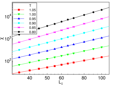
To test the finite-size behavior (3) of the susceptibility, one needs to consider samples having sizes such that is effectively infinite. We have used system sizes and to 100. Figure 1 shows the susceptibility as a function of for several temperatures in the Griffiths region below .


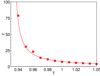
follows a nonuniversal power law in with a temperature-dependent exponent. Simulations for many more temperature values yield analogous results. The value of the exponent extracted from fits to (3) is shown in the right panel of figure 1 for the paramagnetic side of the Griffiths region. can be fitted to the predicted power law , as discussed after (2), giving the estimate
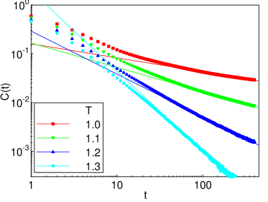
Figure 2 shows the autocorrelation function of the spins as a function of time for several temperatures in the Griffiths phase.

4 Conclusions
In summary, we have performed Monte-Carlo simulations of a randomly layered three-dimensional Heisenberg model. Our numerical results for the magnetic susceptibility and the time autocorrelation function in the paramagnetic Griffiths phase support the infinite-randomness critical point scenario that arises from the strong-disorder renormalization group approach [14]. A full confirmation of the theoretical predictions requires performing a scaling analysis of the infinite-randomness critical point itself, and measuring all three independent critical exponents. This work is in progress.
Experimental verifications of infinite-randomness critical behavior and the accompanying power-law Griffiths singularities have been hard to come by, in particular in higher-dimensional systems. Only very recently, promising measurements have been reported [19, 20] of the quantum phase transitions in CePd1-xRhx and Ni1-xVx. The randomly layered Heisenberg magnet considered here provides an alternative realization of an infinite-randomness critical point. It may be more easily realizable in experiment because the critical point is classical, and samples can be produced by depositing random layers of two different ferromagnetic materials.
This work has been supported in part by the NSF under grant nos. DMR-0339147 and DMR-0906566 and by Research Corporation.
References
References
- [1] Thill M and Huse D A 1995 Physica A 214 321
- [2] Guo M, Bhatt R N and Huse D A 1996 Phys. Rev. B 54 3336
- [3] Rieger H and Young A P 1996 Phys. Rev. B 54 3328
- [4] Fisher D S 1992 Phys. Rev. Lett. 69 534
- [5] Fisher D S 1995 Phys. Rev. B 51 6411
- [6] Vojta T 2003 Phys. Rev. Lett. 90 107202
- [7] Hoyos J A and Vojta T 2008 Phys. Rev. Lett. 100 240601
- [8] Vojta T 2006 J. Phys. A 39 R143
- [9] Vojta T 2010 (Preprint arxiv:1005.2707)
- [10] McCoy B M and Wu T T 1968 Phys. Rev. Lett. 21 549
- [11] McCoy B M and Wu T T 1968 Phys. Rev. 176 631
- [12] McCoy B M and Wu T T 1969 Phys. Rev. 188 982
- [13] McCoy B M 1969 Phys. Rev. Lett. 23 383
- [14] Mohan P, Narayanan R and Vojta T 2010 Phys. Rev. B 81 144407
- [15] Vojta T and Schmalian J 2005 Phys. Rev. B 72 045438
- [16] Hohenberg P C and Halperin B I 1977 Rev. Mod. Phys. 49 435
- [17] Wolff U 1989 Phys. Rev. Lett. 62 361
- [18] Metropolis N, Rosenbluth A, Rosenbluth M and Teller A 1953 J. Chem. Phys. 21 1087
- [19] Westerkamp T, Deppe M, Küchler R, Brando M, Geibel C, Gegenwart P, Pikul A P and Steglich F 2009 Phys. Rev. Lett. 102 206404
- [20] Ubaid-Kassis S, Vojta T and Schroeder A 2010 Phys. Rev. Lett. 104 066402