A Sensor-based Long Baseline Position and Velocity Navigation Filter for Underwater Vehicles

Abstract

This paper presents a novel Long Baseline (LBL) position and velocity navigation filter for underwater vehicles based directly on the sensor measurements. The solution departs from previous approaches as the range measurements are explicitly embedded in the filter design, therefore avoiding inversion algorithms. Moreover, the nonlinear system dynamics are considered to their full extent and no linearizations are carried out whatsoever. The filter error dynamics are globally asymptotically stable (GAS) and it is shown, under simulation environment, that the filter achieves similar performance to the Extended Kalman Filter (EKF) and outperforms linear position and velocity filters based on algebraic estimates of the position obtained from the range measurements.

1 Introduction

Accurate navigation systems are essential for the successful operation of autonomous vehicles. Although there exist alternatives such as terrain-based navigation, most navigation systems contain an Inertial Navigation System (INS) that provides the state of the vehicle by integrating, in open-loop, the information provided by inertial sensors, e.g., accelerometers and rate gyros. Although INS provides very good short term results, its performance necessarily degrades over time, not only due to the integration of sensor noise but also due to sensor bias errors. In order to overcome these drawbacks, aiding devices are considered to correct INS errors. This paper addresses the problem of vehicle navigation using ranges to a set of landmarks disposed in a Long Baseline (LBL) configuration.

Among the myriad of aiding devices, the Global Positioning System (GPS) is a very popular choice, see, e.g., Sukkarieh et al. (1999) Yun et al. (1999), and Vik, B. and Fossen, T. (2001). For underwater vehicles, GPS is not a solution due to the strong attenuation that the electromagnetic field suffers in water. Therefore, other solutions have been sought in the past, including acoustic positioning systems like LBL and Short Baseline (SBL), see Jouffroy and Opderbecke (2004), Kinsey and Whitcomb (2003), Larsen (2001), Larsen (2000), Vaganay et al. (1998), and references therein. In Youngberg (1992) the author proposes a GPS-like system consisting of buoys equipped with DGPS receptors. A related solution, denominated as GPS Intelligent Buoy (GIB) system, is now commercially available, see Thomas (1998). Further work on the GIB underwater positioning system can be found in Alcocer et al. (2007). Position and linear velocity globally asymptotically stable (GAS) filters based on a Ultra-Short Baseline (USBL) positioning system were presented by the authors in Batista et al. (2008). For interesting discussions and more detailed surveys on underwater vehicle navigation and sensing devices see Kinsey et al. (2006) and Leonard et al. (1998).

This paper presents a position and linear velocity navigation filter based on range measurements disposed in a LBL configuration. Traditional solutions resort either to the Extended Kalman Filter (EKF) or to solutions based on position algebraic estimates obtained from the range measurements. The solution presented in the paper departs from previous approaches as the range measurements are explicitly embedded in the filter design, therefore avoiding inversion algorithms. Moreover, the nonlinear system dynamics are considered to their full extent and no linearizations are carried out whatsoever, which allows to show that the filter error dynamics are globally asymptotically stable. Central to the proposed filtering framework is the derivation of a linear time-varying (LTV) system that captures the dynamics of the nonlinear system. The LTV model is achieved through appropriate state augmentation, which is shown to mimic the nonlinear system. Applications of the proposed solution are many and, under simulation environment, it is shown that the filter achieves similar performance to the Extended Kalman Filter (EKF) and outperforms linear position and velocity filters based on position algebraic estimates obtained directly from the range measurements.

The paper is organized as follows. The problem statement and nominal system dynamics are introduced in Section 2, while the filter design is detailed in Section 3. Simulation results are presented in Section 4 and Section 5 summarizes the main conclusions of the paper.

1.1 Notation

Throughout the paper the symbol ${\mathbf{0}}_{n\times m}$ denotes an $n\times m$ matrix of zeros, ${\mathbf{I}}_{n}$ an identity matrix with dimension $n\times n$, and $\rm{diag}({\mathbf{A}}_{1},\ldots,{\mathbf{A}}_{n})$ a block diagonal matrix. When the dimensions are omitted the matrices are assumed of appropriate dimensions. If ${\mathbf{x}}$ and ${\mathbf{y}}$ are two vectors of identical dimensions, ${\mathbf{x}}\times{\mathbf{y}}$ and ${\mathbf{x}}\cdot{\mathbf{y}}$ represent the cross and inner products, respectively.

2 Problem Statement

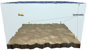
Consider an underwater vehicle moving in a scenario where there is a set of fixed landmarks installed in a Long Baseline configuration and suppose that the vehicle measures the range to each of the landmarks, as depicted in Fig. 1.

Figure 1: Mission Scenario

Further assume that the vehicle is equipped with an Inertial Measurement Unit (IMU), consisting of two triads of orthogonally mounted accelerometers and rate gyros, and an Attitude and Heading Reference System (AHRS). The problem considered in the paper is the design of a sensor-based globally asymptotically stable filter to estimate the position and linear velocity of the vehicle.

2.1 System Dynamics

In order to detail the problem framework, let $\{I\}$ denote an inertial reference coordinate frame and $\{B\}$ a coordinate frame attached to the vehicle, commonly denominated as the body-fixed coordinate frame. The linear motion of the vehicle is described by

$$\dot{{\mathbf{p}}}(t)={\mathbf{R}}(t){\mathbf{v}}(t),$$ (1)

where ${\mathbf{p}}\in{\mathbb{R}}^{3}$ denotes the inertial position of the vehicle, ${\mathbf{v}}\in{\mathbb{R}}^{3}$ is the velocity of the vehicle relative to $\{I\}$ and expressed in body-fixed coordinates, and ${\mathbf{R}}$ is the rotation matrix from $\{B\}$ to $\{I\}$, which satisfies $\dot{{\mathbf{R}}}(t)={\mathbf{R}}(t){\mathbf{S}}\left({\mbox{\boldmath$\omega$}}(t)\right)$, where ${\mbox{\boldmath$\omega$}}\in{\mathbb{R}}^{3}$ is the angular velocity of $\{B\}$, expressed in body-fixed coordinates, and ${\mathbf{S}}\left({\mbox{\boldmath$\omega$}}\right)$ is the skew-symmetric matrix such that ${\mathbf{S}}\left({\mbox{\boldmath$\omega$}}\right){\mbox{\boldmath$x$}}$ is the cross product ${\mbox{\boldmath$\omega$}}\times{\mbox{\boldmath$x$}}$.

The AHRS provides the attitude rotation matrix ${\mathbf{R}}$ and the angular velocity $\omega$, while the IMU, assumed mounted at the center of mass of the vehicle, measures the linear acceleration ${\mathbf{a}}$, which satisfies

$${\mathbf{a}}(t)=\dot{{\mathbf{v}}}(t)+{\mathbf{S}}\left({\mbox{\boldmath$\omega$}}(t)\right){\mathbf{v}}(t)-{\mathbf{g}}(t),$$ (2)

where ${\mathbf{g}}\in{\mathbb{R}}^{3}$ denotes the acceleration of gravity, expressed in body-fixed coordinates. Ideal accelerometers would not measure the gravitational term but in practice this term must be considered due to the inherent physics of the accelerometers, see Kelly (1994) for further details. Since the magnitude of ${\mathbf{g}}$ is usually well known, it would be possible to cancel this term in (2) as the attitude of the vehicle is measured. However, even small errors on ${\mathbf{R}}$ would lead to large errors in the acceleration compensation. Therefore, the acceleration of gravity is considered here as unknown state, in addition to ${\mathbf{p}}$ and ${\mathbf{v}}$. The term ${\mathbf{S}}\left({\mbox{\boldmath$\omega$}}(t)\right){\mathbf{v}}(t)$ corresponds to the Coriolis acceleration and cannot be neglected, particularly for vehicles that execute aggressive maneuvers. Finally, let ${\mathbf{s}}_{i}\in{\mathbb{R}}^{3},\,i=1,\,\ldots,\,n_{\scriptscriptstyle L},$ denote the inertial positions of the landmarks. Then, the range measurements are given by

$$r_{i}(t)=\left\|{\mathbf{s}}_{i}-{\mathbf{p}}(t)\right\|.$$ (3)

The derivative of the velocity can be written, from (2), as

$$\dot{{\mathbf{v}}}(t)={\mathbf{a}}(t)-{\mathbf{S}}\left({\mbox{\boldmath$\omega$}}(t)\right){\mathbf{v}}(t)+{\mathbf{g}}(t).$$ (4)

The derivative of ${\mathbf{g}}$, assuming that the acceleration of gravity is constant in inertial coordinates, is given by

$$\dot{{\mathbf{g}}}(t)=-{\mathbf{S}}\left({\mbox{\boldmath$\omega$}}(t)\right){\mathbf{g}}(t).$$ (5)

Combining (1) and (3)-(5) yields the nonlinear system

$$\left\{\begin{array}[]{l}\dot{{\mathbf{p}}}(t)={\mathbf{R}}(t){\mathbf{v}}(t)\\ \dot{{\mathbf{v}}}(t)={\mathbf{a}}(t)-{\mathbf{S}}\left({\mbox{\boldmath$\omega$}}(t)\right){\mathbf{v}}(t)+{\mathbf{g}}(t)\\ \dot{{\mathbf{g}}}(t)=-{\mathbf{S}}\left({\mbox{\boldmath$\omega$}}(t)\right){\mathbf{g}}(t)\\ r_{1}(t)=\left\|{\mathbf{s}}_{1}-{\mathbf{p}}(t)\right\|\\ \vdots\\ r_{n_{\scriptscriptstyle L}}(t)=\left\|{\mathbf{s}}_{n_{\scriptscriptstyle L}}-{\mathbf{p}}(t)\right\|\end{array}\right..$$ (6)

The problem considered in the paper is the design of a filter for (6) assuming noisy measurements.

In the accelerometer measurements (2) it was not considered accelerometer bias. Its inclusion in the system dynamics is trivial but the observability analysis would result even more tedious. Nevertheless, the observability of linear motion quantities considering accelerometer bias was previously studied by the authors in Batista et al. (2009a) and it is rather straightforward to conclude about the necessary (and sufficient) conditions for observability of the system considering also accelerometer bias. For the sake of simplicity and clarity of presentation, which focuses on the novel Long Baseline solution, the accelerometer is assumed to be calibrated in this paper and the overall system analysis and design will be considered elsewhere.

2.2 Long Baseline Configuration

Long Baseline acoustic configurations have been widely used in the past in the design of navigation systems. In the remainder of the paper the following assumption is considered:

Assumption 1

There exists at least 4 noncoplanar landmarks.

When there exist at least 4 noncoplanar landmarks, it is always possible to determine the position of the vehicle from the range measurements. When there are fewer measurements that may not always be possible. For example, for a static vehicle and 3 landmarks, there exist two possible solutions. Although it is assumed that there are at least 4 noncoplanar landmarks, the proposed solution is general and a more detailed discussion on different LBL configurations will be presented in the sequel.

3 Filter Design

This section presents the main results of the paper. Firstly, a state transformation is applied, in Section 3.1, to reduce the complexity of the system dynamics. Afterwards, state augmentation is proposed, in Section 3.2, in order to derive sensor-based deterministic system dynamics, and in Section 3.3 the observability of the resulting system is analyzed. The design of a Kalman filter is detailed in Section 3.4 and finally, in Section 3.5, some practical considerations are presented.

3.1 State Transformation

Let ${\mathbf{T}}(t):=\rm{diag}\left({\mathbf{I}},{\mathbf{R}}(t),{\mathbf{R}}(t)\right)$ and consider the state transformation

$$\left[\begin{array}[]{c}{\mathbf{x}}_{1}(t)\\ {\mathbf{x}}_{2}(t)\\ {\mathbf{x}}_{3}(t)\end{array}\right]:={\mathbf{T}}(t)\left[\begin{array}[]{c}{\mathbf{p}}(t)\\ {\mathbf{v}}(t)\\ {\mathbf{g}}(t)\end{array}\right],$$ (7)

which is a Lyapunov state transformation previously used by the authors, see Batista et al. (2009b). The new system dynamics are given by

$$\left\{\begin{array}[]{l}\dot{{\mathbf{x}}}_{1}(t)={\mathbf{x}}_{2}(t)\\ \dot{{\mathbf{x}}}_{2}(t)={\mathbf{x}}_{3}(t)+{\mathbf{u}}(t)\\ \dot{{\mathbf{x}}}_{3}(t)={\mathbf{0}}\\ r_{1}(t)=\left\|{\mathbf{s}}_{1}-{\mathbf{x}}_{1}(t)\right\|\\ \vdots\\ r_{n_{\scriptscriptstyle L}}(t)=\left\|{\mathbf{s}}_{n_{\scriptscriptstyle L}}-{\mathbf{x}}_{1}(t)\right\|\end{array}\right.,$$ (8)

where ${\mathbf{u}}(t):={\mathbf{R}}(t){\mathbf{a}}(t)$. Notice that, as (7) is a Lyapunov state transformation, all observability properties are preserved Brockett (1970). The advantage of considering the state transformation (7) is that the new system is time invariant, although it is still nonlinear.

3.2 State Augmentation

To derive a linear system that mimics the dynamics of the nonlinear system (8), define $n_{\scriptscriptstyle L}+4$ additional scalar state variables as

$$\left\{\begin{array}[]{l}x_{4}(t):=r_{1}(t)\\ \vdots\\ x_{n_{\scriptscriptstyle L}+3}(t):=r_{n_{\scriptscriptstyle L}}(t)\\ x_{n_{\scriptscriptstyle L}+4}(t):={\mathbf{x}}_{1}(t)\cdot{\mathbf{x}}_{2}(t)\\ x_{n_{\scriptscriptstyle L}+5}(t):={\mathbf{x}}_{1}(t)\cdot{\mathbf{x}}_{3}(t)+\left\|{\mathbf{x}}_{2}(t)\right\|^{2}\\ x_{n_{\scriptscriptstyle L}+6}:={\mathbf{x}}_{2}(t)\cdot{\mathbf{x}}_{3}(t)\\ x_{n_{\scriptscriptstyle L}+7}(t):=\left\|{\mathbf{x}}_{3}(t)\right\|^{2}\end{array}\right.$$

and denote by

$${\mbox{\boldmath$x$}}(t)=\left[{\mathbf{x}}_{1}^{T}(t)\,{\mathbf{x}}_{2}^{T}(t)\,{\mathbf{x}}_{3}^{T}(t)\,x_{4}(t)\,\ldots\,x_{n_{\scriptscriptstyle L}+7}\right]^{T}\in{\mathbb{R}}^{n},$$

$n=13+n_{\scriptscriptstyle L}$, the augmented state. It is easy to verify that the augmented dynamics can be written as

$$\dot{{\mbox{\boldmath$x$}}}(t)={\mathbf{A}}(t){\mbox{\boldmath$x$}}(t)+{\mathbf{B}}{\mathbf{u}}(t)\\$$

where

$${\mathbf{A}}(t)=\left[\!\begin{array}[]{cccccccccc}{\mathbf{0}}\!&\!{\mathbf{I}}\!&\!{\mathbf{0}}\!&\!{\mathbf{0}}\!&\!\ldots\!&\!{\mathbf{0}}\!&\!{\mathbf{0}}\!&\!{\mathbf{0}}\!&\!{\mathbf{0}}\!&\!{\mathbf{0}}\\ {\mathbf{0}}\!&\!{\mathbf{0}}\!&\!{\mathbf{I}}\!&\!{\mathbf{0}}\!&\!\ldots\!&\!{\mathbf{0}}\!&\!{\mathbf{0}}\!&\!{\mathbf{0}}\!&\!{\mathbf{0}}\!&\!{\mathbf{0}}\\ {\mathbf{0}}\!&\!{\mathbf{0}}\!&\!{\mathbf{0}}\!&\!{\mathbf{0}}\!&\!\ldots\!&\!{\mathbf{0}}\!&\!{\mathbf{0}}\!&\!{\mathbf{0}}\!&\!{\mathbf{0}}\!&\!{\mathbf{0}}\\ {\mathbf{0}}\!&\!-\frac{{\mathbf{s}}_{1}^{T}}{r_{1}\left(t\right)}\!&\!{\mathbf{0}}\!&\!0\!&\!\ldots\!&\!0\!&\!\frac{1}{r_{1}\left(t\right)}\!&\!0\!&\!0\!&\!0\\ \vdots\!&\!\vdots\!&\!\vdots\!&\!\vdots\!&\!\!&\!\vdots\!&\!\vdots\!&\!\vdots\!&\!\vdots\!&\!\vdots\\ {\mathbf{0}}\!&\!-\frac{{\mathbf{s}}_{n_{L}}^{T}}{r_{n_{\scriptscriptstyle L}}\left(t\right)}\!&\!{\mathbf{0}}\!&\!0\!&\!\ldots\!&\!0\!&\!\frac{1}{r_{n_{L}}\left(t\right)}\!&\!0\!&\!0\!&\!0\\ {\mathbf{u}}^{T}(t)\!&\!{\mathbf{0}}\!&\!{\mathbf{0}}\!&\!0\!&\!\ldots\!&\!0\!&\!0\!&\!1\!&\!0\!&\!0\\ {\mathbf{0}}\!&\!2{\mathbf{u}}^{T}(t)\!&\!{\mathbf{0}}\!&\!0\!&\!\ldots\!&\!0\!&\!0\!&\!0\!&\!3\!&\!0\\ {\mathbf{0}}\!&\!{\mathbf{0}}\!&\!{\mathbf{u}}^{T}(t)\!&\!0\!&\!\ldots\!&\!0\!&\!0\!&\!0\!&\!0\!&\!1\\ {\mathbf{0}}\!&\!{\mathbf{0}}\!&\!{\mathbf{0}}\!&\!0\!&\!\ldots\!&\!0\!&\!0\!&\!0\!&\!0\!&\!0\end{array}\!\right]$$ (19)

and ${\mathbf{B}}=\left[{\mathbf{0}}\,{\mathbf{I}}\,{\mathbf{0}}\,0\,\ldots 0\right]^{T}$.

In order to complete the augmented system dynamics, notice first that the states $x_{4},\,\ldots,\,x_{3+n_{\scriptscriptstyle L}}$ are measured. In addition to that, it is straightforward to show that

$$\frac{2\left({\mathbf{s}}_{i}-{\mathbf{s}}_{j}\right)\cdot{\mathbf{p}}(t)}{r_{i}(t)+r_{j}(t)}+r_{i}(t)-r_{j}(t)=\frac{\left\|{\mathbf{s}}_{i}\right\|^{2}-\left\|{\mathbf{s}}_{j}\right\|^{2}}{r_{i}(t)+r_{j}(t)}$$

or, equivalently,

$$\frac{2\left({\mathbf{s}}_{i}-{\mathbf{s}}_{j}\right)\cdot{\mathbf{x}}_{1}(t)}{r_{i}(t)+r_{j}(t)}+x_{3+i}(t)-x_{3+j}(t)=\frac{\left\|{\mathbf{s}}_{i}\right\|^{2}-\left\|{\mathbf{s}}_{j}\right\|^{2}}{r_{i}(t)+r_{j}(t)},$$ (20)

where the right side of (20) is known and the left side depends on the system state. Discarding the original nonlinear system output, it is possible to write an augmented system output as

$$\left\{\!\!\!\begin{array}[]{l}y_{1}(t)=x_{4}(t)\\ \vdots\\ y_{n_{\scriptscriptstyle L}}(t)=x_{3+n_{\scriptscriptstyle L}}(t)\\ y_{n_{\scriptscriptstyle L}+1}=\frac{2\left({\mathbf{s}}_{1}-{\mathbf{s}}_{2}\right)\cdot{\mathbf{x}}_{1}(t)}{r_{1}(t)+r_{2}(t)}+x_{3+1}(t)-x_{3+2}(t)\\ y_{n_{\scriptscriptstyle L}+2}=\frac{2\left({\mathbf{s}}_{1}-{\mathbf{s}}_{3}\right)\cdot{\mathbf{x}}_{1}(t)}{r_{1}(t)+r_{3}(t)}+x_{3+1}(t)-x_{3+3}(t)\\ \vdots\\ y_{n_{\scriptscriptstyle L}+C_{2}^{n_{\scriptscriptstyle L}}-1}=\frac{2\left({\mathbf{s}}_{n_{\scriptscriptstyle L}-2}\!-\!{\mathbf{s}}_{n_{\scriptscriptstyle L}}\right)\!\cdot\!{\mathbf{x}}_{1}(t)}{r_{n_{\scriptscriptstyle L}-2}(t)+r_{n_{\scriptscriptstyle L}}(t)}+x_{3+{n_{\scriptscriptstyle L}-2}}(t)\!-\!x_{3+{n_{\scriptscriptstyle L}}}(t)\\ y_{n_{\scriptscriptstyle L}+C_{2}^{n_{\scriptscriptstyle L}}}=\frac{2\left({\mathbf{s}}_{n_{\scriptscriptstyle L}-1}\!-\!{\mathbf{s}}_{n_{\scriptscriptstyle L}}\right)\!\cdot\!{\mathbf{x}}_{1}(t)}{r_{n_{\scriptscriptstyle L}-1}(t)+r_{n_{\scriptscriptstyle L}}(t)}+x_{3+{n_{\scriptscriptstyle L}-1}}(t)\!-\!x_{3+{n_{\scriptscriptstyle L}}}(t)\end{array}\right.\!\!\!\!\!\!,$$

where $C_{2}^{n_{\scriptscriptstyle L}}$ is the number of 2-combinations of $n_{\scriptscriptstyle L}$ elements, i.e., $C_{2}^{n_{\scriptscriptstyle L}}=\frac{\left(n_{\scriptscriptstyle L}-1\right)n_{\scriptscriptstyle L}}{2}$. In compact form, the augmented system dynamics are given by

$$\left\{\begin{array}[]{l}\dot{{\mbox{\boldmath$x$}}}(t)={\mathbf{A}}(t){\mbox{\boldmath$x$}}(t)+{\mathbf{B}}{\mathbf{u}}(t)\\ {\mathbf{y}}(t)={\mathbf{C}}(t){\mbox{\boldmath$x$}}(t)\end{array}\right.,$$ (21)

where

$${\mathbf{C}}(t)=\left[\begin{array}[]{ccc|c|c}{\mathbf{0}}_{n_{\scriptscriptstyle L}\times 3}&{\mathbf{0}}_{n_{\scriptscriptstyle L}\times 3}&{\mathbf{0}}_{n_{\scriptscriptstyle L}\times 3}&{\mathbf{I}}_{n_{\scriptscriptstyle L}}&{\mathbf{0}}_{n_{\scriptscriptstyle L}\times 4}\\ \hline\cr{\mathbf{C}}_{1}(t)&{\mathbf{0}}_{C_{2}^{n_{\scriptscriptstyle L}}\times 3}&{\mathbf{0}}_{C_{2}^{n_{\scriptscriptstyle L}}\times 3}&{\mathbf{C}}_{2}&{\mathbf{0}}_{C_{2}^{n_{\scriptscriptstyle L}}\times 4}\end{array}\right],$$ (22)

$${\mathbf{C}}_{1}(t)=\left[\begin{array}[]{c}\frac{2\left({\mathbf{s}}_{1}-{\mathbf{s}}_{2}\right)^{T}}{r_{1}(t)+r_{2}(t)}\\ \frac{2\left({\mathbf{s}}_{1}-{\mathbf{s}}_{3}\right)^{T}}{r_{1}(t)+r_{3}(t)}\\ \vdots\\ \frac{2\left({\mathbf{s}}_{n_{\scriptscriptstyle L}-2}-{\mathbf{s}}_{n_{\scriptscriptstyle L}}\right)^{T}}{r_{n_{\scriptscriptstyle L}-2}(t)+r_{n_{\scriptscriptstyle L}}(t)}\\ \frac{2\left({\mathbf{s}}_{n_{\scriptscriptstyle L}-1}-{\mathbf{s}}_{n_{\scriptscriptstyle L}}\right)^{T}}{r_{n_{\scriptscriptstyle L}-1}(t)+r_{n_{\scriptscriptstyle L}}(t)}\end{array}\right]\in{\mathbb{R}}^{n_{\scriptscriptstyle L}\times 3},$$

and

$${\mathbf{C}_{2}}=\left[\begin{array}[]{ccccccc}1&-1&0&\ldots&\ldots&\ldots&0\\ 1&0&-1&0&\ldots&\ldots&0\\ &&&\vdots\\ 0&\ldots&\ldots&0&1&0&-1\\ 0&\ldots&\ldots&\ldots&0&1&-1\end{array}\right]\in{\mathbb{R}}^{C_{2}^{n_{\scriptscriptstyle L}}\times n_{\scriptscriptstyle L}}$$

is the matrix that encodes all the possible combinations of differences of pairs of ranges.

The dynamic system (21) can be regarded as a linear time-varying system, even though the system matrices ${\mathbf{A}}(t)$ and ${\mathbf{C}}(t)$ depend explicitly on the system input and output, as evidenced by (19) and (22). However, these are known signals and therefore pose no problem, other than the fact that the observability of the system may depend on the system input, which does not happen for linear systems whose system matrices do not depend on the system input. Also, notice that there is nothing in (21) imposing

$$\left\{\begin{array}[]{l}r_{1}(t)=\left\|{\mathbf{s}}_{1}-{\mathbf{x}}_{1}(t)\right\|\\ \vdots\\ r_{n_{\scriptscriptstyle L}}(t)=\left\|{\mathbf{s}}_{n_{\scriptscriptstyle L}}-{\mathbf{x}}_{1}(t)\right\|\\ x_{n_{\scriptscriptstyle L}+4}(t)={\mathbf{x}}_{1}(t)\cdot{\mathbf{x}}_{2}(t)\\ x_{n_{\scriptscriptstyle L}+5}(t)={\mathbf{x}}_{1}(t)\cdot{\mathbf{x}}_{3}(t)+\left\|{\mathbf{x}}_{2}(t)\right\|^{2}\\ x_{n_{\scriptscriptstyle L}+6}(t)={\mathbf{x}}_{2}(t)\cdot{\mathbf{x}}_{3}(t)\\ x_{n_{\scriptscriptstyle L}+7}(t)=\left\|{\mathbf{x}}_{3}(t)\right\|^{2}\end{array}\right..$$ (23)

These restrictions could be easily implemented but this form is preferred since it allows to consider the system as linear. However, care must be taken when extrapolating conclusions from the observability of (21) to the observability of (8) or (6). Finally, the following assumption is required so that (19) is well defined, which is not restrictive from the practical point of view since it would make no sense to have the vehicle at the same position of a landmark, where an acoustic transponder is installed.

Assumption 2

The motion of the vehicle is such that

$$\begin{array}[]{cccc}\exists&\forall&:&r_{m}\leq r_{i}(t).\\ r_{m}>0&t>t_{0}\end{array}$$

3.3 Observability Analysis

In the previous section a LTV system was derived that aims to capture the behavior of the original nonlinear system. The analysis of the observability of this LTV system is carried out in this section and its behavior compared with that of the nonlinear system.

In order to proceed with the analysis of the observability of the LTV system (21), it is convenient to compute the observability Gramian associated with the pair $\left({\mathbf{A}}(t),{\mathbf{C}}(t)\right)$ and, in order to do so, the transition matrix associated with the system matrix ${\mathbf{A}}(t)$. Let

$${\mathbf{u}}^{[1]}\!\left(t,t_{\scriptscriptstyle 0}\right)\!:=\int_{t_{\scriptscriptstyle 0}}^{t}{\mathbf{u}}\left(\sigma\right)d\sigma$$

and

$${\mathbf{u}}^{[2]}\!\left(t,t_{0}\right)\!:=\int_{t_{\scriptscriptstyle 0}}^{t}\int_{t_{\scriptscriptstyle 0}}^{\sigma_{1}}{\mathbf{u}}\left(\sigma_{2}\right)d\sigma_{2}d\sigma_{1}.$$

Long, but straightforward, computations show that the transition matrix associated with ${\mathbf{A}}(t)$ is given by

$${\mbox{\boldmath$\phi$}}\left(t,t_{\scriptscriptstyle 0}\right)=\left[\begin{array}[]{ccc}{\mbox{\boldmath$\phi$}}_{\scriptscriptstyle AA}\left(t,t_{\scriptscriptstyle 0}\right)&{\mathbf{0}}&{\mathbf{0}}\\ {\mbox{\boldmath$\phi$}}_{\scriptscriptstyle BA}\left(t,t_{\scriptscriptstyle 0}\right)&{\mathbf{I}}&{\mbox{\boldmath$\phi$}}_{\scriptscriptstyle BC}\left(t,t_{\scriptscriptstyle 0}\right)\\ {\mbox{\boldmath$\phi$}}_{\scriptscriptstyle CA}\left(t,t_{\scriptscriptstyle 0}\right)&{\mathbf{0}}&{\mbox{\boldmath$\phi$}}_{\scriptscriptstyle CC}\left(t,t_{\scriptscriptstyle 0}\right)\end{array}\right],$$

where

$${\mbox{\boldmath$\phi$}}_{\scriptscriptstyle AA}\left(t,t_{\scriptscriptstyle 0}\right)=\left[\begin{array}[]{ccc}{\mathbf{I}}&\left(t-t_{\scriptscriptstyle 0}\right){\mathbf{I}}&\frac{\left(t-t_{\scriptscriptstyle 0}\right)^{2}}{2}{\mathbf{I}}\\ {\mathbf{0}}&{\mathbf{I}}&\left(t-t_{\scriptscriptstyle 0}\right){\mathbf{I}}\\ {\mathbf{0}}&{\mathbf{0}}&{\mathbf{I}}\end{array}\right],$$

$${\mbox{\boldmath$\phi$}}_{\scriptscriptstyle BA}\left(t,t_{\scriptscriptstyle 0}\right)=\left[\begin{array}[]{ccc}{\mbox{\boldmath$\phi$}}_{\scriptscriptstyle BA1}\left(t,t_{\scriptscriptstyle 0}\right)&{\mbox{\boldmath$\phi$}}_{\scriptscriptstyle BA2}\left(t,t_{\scriptscriptstyle 0}\right)&{\mbox{\boldmath$\phi$}}_{\scriptscriptstyle BA3}\left(t,t_{\scriptscriptstyle 0}\right)\end{array}\right],$$

$${\mbox{\boldmath$\phi$}}_{\scriptscriptstyle BA1}\left(t,t_{\scriptscriptstyle 0}\right)=\left[\!\!\!\begin{array}[]{c}\int_{t_{0}}^{t}\frac{\left[{\mathbf{u}}^{[1]}\!\left(\sigma,t_{\scriptscriptstyle 0}\right)\right]^{T}}{r_{1}\left(\sigma\right)}d\sigma\\ \vdots\\ \int_{t_{0}}^{t}\frac{\left[{\mathbf{u}}^{[1]}\!\left(\sigma,t_{\scriptscriptstyle 0}\right)\right]}{r_{n_{\scriptscriptstyle L}}\left(\sigma\right)}d\sigma\\ \end{array}\!\!\!\right]\!\!,$$

$${\mbox{\boldmath$\phi$}}_{\scriptscriptstyle BA2}\left(t,t_{\scriptscriptstyle 0}\right)=$$

$$\left[\!\!\!\begin{array}[]{c}\int_{t_{0}}^{t}\frac{-{\mathbf{s}}_{1}^{T}+\left(\sigma-t_{0}\right)\left[{\mathbf{u}}^{[1]}\!\left(\sigma,t_{0}\right)\right]^{T}+\left[{\mathbf{u}}^{[2]}\!\left(\sigma,t_{0}\right)\right]^{T}}{r_{1}\left(\sigma\right)}d\sigma\\ \vdots\\ \int_{t_{0}}^{t}\frac{-{\mathbf{s}}_{n_{\scriptscriptstyle L}}^{T}+\left(\sigma-t_{0}\right)\left[{\mathbf{u}}^{[1]}\!\left(\sigma,t_{0}\right)\right]^{T}+\left[{\mathbf{u}}^{[2]}\!\left(\sigma,t_{0}\right)\right]^{T}}{r_{n_{\scriptscriptstyle L}}\left(\sigma\right)}d\sigma\end{array}\!\!\!\right]\!\!,$$

$${\mbox{\boldmath$\phi$}}_{\scriptscriptstyle BA3}\left(t,t_{\scriptscriptstyle 0}\right)=$$

$$\left[\!\!\!\begin{array}[]{c}\int_{t_{0}}^{t}\!\!\left(\sigma-t_{\scriptscriptstyle 0}\right)\frac{-{\mathbf{s}}_{1}^{T}+\frac{\left(\sigma-t_{0}\right)}{2}\left[{\mathbf{u}}^{[1]}\!\left(\sigma,t_{0}\right)\right]^{T}+\left[{\mathbf{u}}^{[2]}\!\left(\sigma,t_{0}\right)\right]^{T}}{r_{1}\left(\sigma\right)}d\sigma\\ \vdots\\ \int_{t_{0}}^{t}\!\!\left(\sigma-t_{\scriptscriptstyle 0}\right)\frac{-{\mathbf{s}}_{n_{\scriptscriptstyle L}}^{T}+\frac{\left(\sigma-t_{0}\right)}{2}\left[{\mathbf{u}}^{[1]}\!\left(\sigma,t_{0}\right)\right]^{T}+\left[{\mathbf{u}}^{[2]}\!\left(\sigma,t_{0}\right)\right]^{T}}{r_{n_{\scriptscriptstyle L}}\left(\sigma\right)}d\sigma\\ \end{array}\!\!\!\right]\!\!,$$

$${\mbox{\boldmath$\phi$}}_{\scriptscriptstyle BC}\left(t,t_{\scriptscriptstyle 0}\right)=$$

$$\!\!\!\left[\!\!\!\begin{array}[]{cccc}\int_{t_{0}}^{t}\!\frac{1}{r_{1}\left(\sigma\right)}d\sigma\!&\!\int_{t_{0}}^{t}\!\frac{\sigma-t_{\scriptscriptstyle 0}}{r_{1}\left(\sigma\right)}d\sigma\!&\!\int_{t_{0}}^{t}\!\frac{3}{2}\frac{\left(\sigma-t_{\scriptscriptstyle 0}\right)^{2}}{r_{1}\left(\sigma\right)}d\sigma\!&\!\int_{t_{0}}^{t}\!\frac{1}{2}\frac{\left(\sigma-t_{\scriptscriptstyle 0}\right)^{3}}{r_{1}\left(\sigma\right)}d\sigma\\ \vdots&\vdots&\vdots&\vdots\\ \int_{t_{0}}^{t}\!\frac{1}{r_{n_{\scriptscriptstyle L}}\!\left(\sigma\right)}d\sigma\!\!&\!\!\int_{t_{0}}^{t}\!\frac{\sigma-t_{\scriptscriptstyle 0}}{r_{n_{\scriptscriptstyle L}}\!\left(\sigma\right)}d\sigma\!\!&\!\!\int_{t_{0}}^{t}\!\frac{3}{2}\frac{\left(\sigma-t_{\scriptscriptstyle 0}\right)^{2}}{r_{n_{\scriptscriptstyle L}}\!\left(\sigma\right)}d\sigma\!\!&\!\!\int_{t_{0}}^{t}\!\frac{1}{2}\frac{\left(\sigma-t_{\scriptscriptstyle 0}\right)^{3}}{r_{n_{\scriptscriptstyle L}}\!\left(\sigma\right)}d\sigma\\ \end{array}\!\!\!\right]\!\!,$$

and ${\mbox{\boldmath$\phi$}}_{\scriptscriptstyle CA}\left(t,t_{\scriptscriptstyle 0}\right)$ and ${\mbox{\boldmath$\phi$}}_{\scriptscriptstyle CC}\left(t,t_{\scriptscriptstyle 0}\right)$ are omitted for the sake of simplicity, as they are not required in the sequel. The observability Gramian associated with the pair $\left({\mathbf{A}}(t),{\mathbf{C}}(t)\right)$ is simply given by

$${\mbox{\boldmath$\mathcal{W}$}}\left(t_{0},t_{f}\right)=\int_{t_{0}}^{t_{f}}{{\mbox{\boldmath$\phi$}}^{T}\left(t,t_{0}\right){\mathbf{C}}^{T}(t){\mathbf{C}}(t){\mbox{\boldmath$\phi$}}\left(t,t_{0}\right)dt}.$$

The following theorem establishes the observability of the LTV system (21).

Theorem 1

The linear time-varying system (21) is observable on $\left[t_{0},t_{f}\right]$, $t_{0}<t_{f}$.

The proof follows by contradiction. Suppose that the LTV system (21) is not observable on ${\mathcal{I}}:=\left[t_{0},t_{f}\right]$. Then, there exists a nonnull vector ${\mathbf{d}}\in{\mathbb{R}}^{13+n_{\scriptscriptstyle L}}$

$${\mathbf{d}}=\left[{\mathbf{d}}_{1}^{T}{\mathbf{d}}_{2}^{T}{\mathbf{d}}_{3}^{T}{\mathbf{d}}_{4}^{T}d_{5}d_{6}d_{7}d_{8}\right]^{T},$$

with ${\mathbf{d}}_{1},\,{\mathbf{d}}_{2},\,{\mathbf{d}}_{3}\in{\mathbb{R}}^{3}$, ${\mathbf{d}}_{4}\in{\mathbb{R}}^{n_{\scriptscriptstyle L}}$, $d_{5},\,\ldots,\,d_{8}\in{\mathbb{R}}$, such that ${\mathbf{d}}^{T}{\mbox{\boldmath$\mathcal{W}$}}\left(t_{0},t\right){\mathbf{d}}=0$ for all $t\in{\mathcal{I}}$ or, equivalently,

$$\int_{t_{\scriptscriptstyle 0}}^{t}\left\|{\mathbf{C}}\left(\tau\right){\mbox{\boldmath$\phi$}}\left(\tau,t_{\scriptscriptstyle 0}\right){\mathbf{d}}\right\|^{2}d\tau=0.$$ (27)

Taking the time derivative of (27) yields

$$\left\|{\mathbf{C}}\left(t\right){\mbox{\boldmath$\phi$}}\left(t,t_{\scriptscriptstyle 0}\right){\mathbf{d}}\right\|^{2}=0,$$

which implies, in particular, that

$${\mathbf{C}}\left(t\right){\mbox{\boldmath$\phi$}}\left(t,t_{\scriptscriptstyle 0}\right){\mathbf{d}}=0$$ (28)

for all $t\in{\mathcal{I}}$. Substituting $t=t_{\scriptscriptstyle 0}$ in (28) gives

$$\left[\begin{array}[]{c}{\mathbf{d}}_{4}\\ {\mathbf{C}}_{1}\left(t_{\scriptscriptstyle 0}\right){\mathbf{d}}_{1}+{\mathbf{C}}_{2}{\mathbf{d}}_{4}\end{array}\right]={\mathbf{0}}$$ (29)

which implies immediately that

$${\mathbf{d}}_{4}={\mathbf{0}}.$$ (30)

Substituting (30) in (29) gives

$$\left[\begin{array}[]{c}\frac{2}{r_{1}\left(t_{0}\right)+r_{2}\left(t_{0}\right)}\left({\mathbf{s}}_{1}-{\mathbf{s}}_{2}\right)^{T}\\ \frac{2}{r_{1}\left(t_{0}\right)+r_{3}\left(t_{0}\right)}\left({\mathbf{s}}_{1}-{\mathbf{s}}_{3}\right)^{T}\\ \vdots\\ \frac{2}{r_{n_{\scriptscriptstyle L}-2}\left(t_{0}\right)+r_{n_{\scriptscriptstyle L}}\left(t_{0}\right)}\left({\mathbf{s}}_{n_{\scriptscriptstyle L}-2}-{\mathbf{s}}_{n_{\scriptscriptstyle L}}\right)^{T}\\ \frac{2}{r_{n_{\scriptscriptstyle L}-1}\left(t_{0}\right)+r_{n_{\scriptscriptstyle L}}\left(t_{0}\right)}\left({\mathbf{s}}_{n_{\scriptscriptstyle L}-1}-{\mathbf{s}}_{n_{\scriptscriptstyle L}}\right)^{T}\end{array}\right]{\mathbf{d}}_{1}={\mathbf{0}}.$$ (31)

It is straightforward to show that, under Assumption 1, the only solution of (31) is

$${\mathbf{d}}_{1}={\mathbf{0}}.$$ (32)

Now, from (28), it is possible to write

$$\frac{d}{dt}\left[{\mathbf{C}}\left(t\right){\mbox{\boldmath$\phi$}}\left(t,t_{\scriptscriptstyle 0}\right){\mathbf{d}}\right]={\mathbf{0}}$$ (33)

for all $t\in{\mathcal{I}}$. Expanding (33), and considering (30) and (32), allows to write

$$\frac{-{\mathbf{s}}_{i}^{T}{\mathbf{d}}_{2}+\left(t-t_{0}\right)\left[{\mathbf{u}}^{[1]}\!\left(t,t_{0}\right)\right]^{T}{\mathbf{d}}_{2}+\left[{\mathbf{u}}^{[2]}\!\left(t,t_{0}\right)\right]^{T}{\mathbf{d}}_{2}}{r_{i}\left(t\right)}$$

$$+\left(t-t_{\scriptscriptstyle 0}\right)\frac{-{\mathbf{s}}_{i}^{T}{\mathbf{d}}_{3}+\frac{\left(t-t_{0}\right)}{2}\left[{\mathbf{u}}^{[1]}\!\left(t,t_{0}\right)\right]^{T}{\mathbf{d}}_{3}+\left[{\mathbf{u}}^{[2]}\!\left(t,t_{0}\right)\right]^{T}{\mathbf{d}}_{3}}{r_{i}\left(t\right)}$$

$$+\frac{1}{r_{i}\left(t\right)}d_{5}+\frac{t-t_{\scriptscriptstyle 0}}{r_{i}\left(t\right)}d_{6}+\frac{3}{2}\frac{\left(t-t_{\scriptscriptstyle 0}\right)^{2}}{r_{i}\left(t\right)}d_{7}+\frac{1}{2}\frac{\left(t-t_{\scriptscriptstyle 0}\right)^{3}}{r_{i}\left(t\right)}d_{8}=0$$

for all $i=1,\,\ldots,\,n_{\scriptscriptstyle L}$, $t\in I$ or, equivalently,

$$\left.-{\mathbf{s}}_{i}^{T}{\mathbf{d}}_{2}+\left(t-t_{0}\right)\left[{\mathbf{u}}^{[1]}\!\left(t,t_{0}\right)\right]^{T}{\mathbf{d}}_{2}+\left[{\mathbf{u}}^{[2]}\!\left(t,t_{0}\right)\right]^{T}{\mathbf{d}}_{2}\right.$$

$$\left.-\left(t-t_{\scriptscriptstyle 0}\right){\mathbf{s}}_{i}^{T}{\mathbf{d}}_{3}+\frac{\left(t-t_{0}\right)^{2}}{2}\left[{\mathbf{u}}^{[1]}\!\left(t,t_{0}\right)\right]^{T}{\mathbf{d}}_{3}\right.$$

$$+\left(t-t_{0}\right)\left[{\mathbf{u}}^{[2]}\!\left(t,t_{0}\right)\right]^{T}{\mathbf{d}}_{3}+d_{5}+\left(t-t_{\scriptscriptstyle 0}\right)d_{6}$$

$$+\frac{3}{2}\left(t-t_{\scriptscriptstyle 0}\right)^{2}d_{7}+\frac{1}{2}\left(t-t_{\scriptscriptstyle 0}\right)^{3}d_{8}=0.$$ (34)

Substituting $t=t_{0}$ in (34) gives

$$\left[\begin{array}[]{cc}-{\mathbf{s}}_{1}^{T}&1\\ -{\mathbf{s}}_{2}^{T}&1\\ \vdots\\ -{\mathbf{s}}_{n_{\scriptscriptstyle L}-1}^{T}&1\\ -{\mathbf{s}}_{n_{\scriptscriptstyle L}}^{T}&1\end{array}\right]\left[\begin{array}[]{c}{\mathbf{d}}_{2}\\ d_{5}\end{array}\right]={\mathbf{0}}.$$ (35)

Again, it is straightforward to show that, under Assumption 1, the only solution of (35) is

$$\left\{\begin{array}[]{l}{\mathbf{d}}_{2}={\mathbf{0}}\\ d_{5}=0\end{array}\right..$$ (36)

Now, considering (36) in (34) and taking its time derivative gives

$$\left.-{\mathbf{s}}_{i}^{T}{\mathbf{d}}_{3}+\frac{\left(t-t_{0}\right)^{2}}{2}\left[{\mathbf{u}}\left(t\right)\right]^{T}{\mathbf{d}}_{3}+\left(t-t_{0}\right)\left[{\mathbf{u}}^{[1]}\!\left(t,t_{0}\right)\right]^{T}{\mathbf{d}}_{3}\right.$$

$$+\left(t-t_{0}\right)\left[{\mathbf{u}}^{[1]}\!\left(t,t_{0}\right)\right]^{T}{\mathbf{d}}_{3}+\left[{\mathbf{u}}^{[2]}\!\left(t,t_{0}\right)\right]^{T}{\mathbf{d}}_{3}+d_{6}$$

$$+3\left(t-t_{\scriptscriptstyle 0}\right)d_{7}+\frac{3}{2}\left(t-t_{\scriptscriptstyle 0}\right)^{2}d_{8}=0$$ (37)

for all $i=1,\,\ldots,\,n_{\scriptscriptstyle L}$ and $t\in I$. With $t=t_{0}$ in (37),

$$\left[\begin{array}[]{cc}-{\mathbf{s}}_{1}^{T}&1\\ -{\mathbf{s}}_{2}^{T}&1\\ \vdots\\ -{\mathbf{s}}_{n_{\scriptscriptstyle L}-1}^{T}&1\\ -{\mathbf{s}}_{n_{\scriptscriptstyle L}}^{T}&1\end{array}\right]\left[\begin{array}[]{c}{\mathbf{d}}_{3}\\ d_{6}\end{array}\right]={\mathbf{0}}.$$ (38)

Again, under Assumption 1, the only solution of (38) is

$$\left\{\begin{array}[]{l}{\mathbf{d}}_{3}={\mathbf{0}}\\ d_{6}=0\end{array}\right..$$ (39)

Finally, substituting (39) in (37) gives

$$3\left(t-t_{\scriptscriptstyle 0}\right)d_{7}+\frac{3}{2}\left(t-t_{\scriptscriptstyle 0}\right)^{2}d_{8}=0$$ (40)

for all $t\in I$. Since $t-t_{0}$ and $\left(t-t_{0}\right)^{2}$ are linearly independent functions, the only solution of (40) is $d_{7}=d_{8}=0$. But that contradicts the hypothesis that there exists a nonnull vector ${\mathbf{d}}$ such that (27) is true. Therefore, the LTV system (21) is observable.

The fact that (21) is observable does not mean that the nonlinear system (8) is observable nor that an observer for (21) is also an observer for (8), as there is nothing in the system dynamics (21) imposing the algebraic restrictions (23). However, this turns out to be true, as shown in the following theorem.

Theorem 2

The nonlinear system (8) is observable in the sense that, given the output $\left\{{\mathbf{y}}(t),\,t\in\left[t_{0},t_{f}\right]\right\}$ and the input $\left\{{\mathbf{u}}(t),\,t\in\left[t_{0},t_{f}\right]\right\}$, the initial state ${\mathbf{x}}\left(t_{0}\right)=\left[{\mathbf{x}}_{1}^{T}\left(t_{0}\right)\,{\mathbf{x}}_{2}^{T}\left(t_{0}\right)\,{\mathbf{x}}_{3}^{T}\left(t_{0}\right)\right]^{T}$ is uniquely defined. Moreover, a state observer for the LTV system (21) with globally asymptotically stable error dynamics is also a state observer for the nonlinear system (8), with globally asymptotically stable error dynamics.

It has been shown, in Theorem 1, that the LTV system (21) is observable. Therefore, given the output $\left\{{\mathbf{y}}(t),\,t\in\left[t_{0},t_{f}\right]\right\}$ and the input $\left\{{\mathbf{u}}(t),\,t\in\left[t_{0},t_{f}\right]\right\}$, the initial state of (21) is uniquely defined. Let

$${\mathbf{z}}\left(t_{0}\right)=\left[{\mathbf{z}}_{1}^{T}\left(t_{0}\right){\mathbf{z}}_{2}^{T}\left(t_{0}\right){\mathbf{z}}_{3}^{T}\left(t_{0}\right)z_{4}\left(t_{0}\right)\ldots\\ z_{n_{\scriptscriptstyle L}+7}\left(t_{0}\right)\right]^{T}$$

${\mathbf{z}}_{1},\,{\mathbf{z}}_{2},\,{\mathbf{z}}_{3}\in{\mathbb{R}}^{3}$, $z_{4},\,\ldots,\,z_{n_{\scriptscriptstyle L}+7}\left(t_{0}\right)\in{\mathbb{R}}$, be the initial state of (21) and ${\mathbf{x}}\left(t_{0}\right)=\left[{\mathbf{x}}_{1}^{T}\left(t_{0}\right){\mathbf{x}}_{2}^{T}\left(t_{0}\right){\mathbf{x}}_{3}^{T}\left(t_{0}\right)\right]^{T}$ be the initial state of the nonlinear system (8). It is easy to show that the evolution, for the nonlinear system, of ${\mathbf{x}}_{1}(t)$, is given by

$${\mathbf{x}}_{1}(t) = {\mathbf{x}}_{1}\left(t_{0}\right)+\left(t-t_{0}\right){\mathbf{x}}_{2}\left(t_{0}\right)+\frac{\left(t-t_{0}\right)^{2}}{2}{\mathbf{x}}_{3}\left(t_{0}\right)$$ (41)

$$+{\mathbf{u}}^{[2]}\!\left(t,t_{0}\right),$$

while the output of the nonlinear system satisfies

$$r_{i}^{2}(t)=\left\|{\mathbf{x}}_{1}\left(t_{0}\right)-{\mathbf{s}}_{i}\right\|^{2}+\left(t-t_{0}\right)^{2}\left\|{\mathbf{x}}_{2}\left(t_{0}\right)\right\|^{2}$$

$$+\frac{\left(t-t_{0}\right)^{4}}{4}\left\|{\mathbf{x}}_{3}\left(t_{0}\right)\right\|^{2}+2\left(t-t_{0}\right){\mathbf{x}}_{1}\left(t_{0}\right)\cdot{\mathbf{x}}_{2}\left(t_{0}\right)$$

$$+\left(t-t_{0}\right)^{2}{\mathbf{x}}_{1}\left(t_{0}\right)\cdot{\mathbf{x}}_{3}\left(t_{0}\right)+\left(t-t_{0}\right)^{3}{\mathbf{x}}_{2}\left(t_{0}\right)\cdot{\mathbf{x}}_{3}\left(t_{0}\right)$$

$$-2\left(t-t_{0}\right){\mathbf{s}}_{i}\cdot{\mathbf{x}}_{2}\left(t_{0}\right)-\left(t-t_{0}\right)^{2}{\mathbf{s}}_{i}\cdot{\mathbf{x}}_{3}\left(t_{0}\right)$$

$$+2{\mathbf{x}}_{1}\left(t_{0}\right)\cdot{\mathbf{u}}^{[2]}\!\left(t,t_{0}\right)+2{\mathbf{x}}_{2}\left(t_{0}\right)\cdot\left(t-t_{0}\right){\mathbf{u}}^{[2]}\!\left(t,t_{0}\right)$$

$$+{\mathbf{x}}_{3}\left(t_{0}\right)\cdot\left(t-t_{0}\right)^{2}{\mathbf{u}}^{[2]}\!\left(t,t_{0}\right)+\left\|{\mathbf{u}}^{[2]}\!\left(t,t_{0}\right)\right\|^{2}$$

$$-2{\mathbf{s}}_{i}\cdot{\mathbf{u}}^{[2]}\!\left(t,t_{0}\right).$$ (42)

Therefore, from (41) and (42), it is trivially shown that

$$r_{i}^{2}(t)-r_{j}^{2}(t)+2\left({\mathbf{s}}_{i}-{\mathbf{s}}_{j}\right)\cdot{\mathbf{x}}_{1}(t)=\left\|{\mathbf{x}}_{1}\left(t_{0}\right)-{\mathbf{s}}_{i}\right\|^{2}$$

$$-\left\|{\mathbf{x}}_{1}\left(t_{0}\right)-{\mathbf{s}}_{j}\right\|^{2}+2\left({\mathbf{s}}_{i}-{\mathbf{s}}_{j}\right)\cdot{\mathbf{x}}_{1}\left(t_{0}\right)$$ (43)

for all $i,j\in\left\{1,\,\ldots,\,n_{\scriptscriptstyle L}\right\}$ and $t\in{\mathcal{I}}$. Now, notice that, for the LTV system, multiplying the set of augmented outputs $y_{n_{\scriptscriptstyle L}+1},\,\ldots,\,y_{n_{\scriptscriptstyle L}+C_{2}^{n_{\scriptscriptstyle L}}}$ by the corresponding sums of pair of ranges yields

$$r_{i}^{2}(t)-r_{j}^{2}(t)+2\left({\mathbf{s}}_{i}-{\mathbf{s}}_{j}\right)\cdot{\mathbf{x}}_{1}(t),$$

while its evolution can be shown to satisfy

$$r_{i}^{2}(t)-r_{j}^{2}(t)+2\left({\mathbf{s}}_{i}-{\mathbf{s}}_{j}\right)\cdot{\mathbf{x}}_{1}(t)=z_{3+i}^{2}\left(t_{0}\right)-z_{3+j}^{2}\left(t_{0}\right)$$

$$+2\left({\mathbf{s}}_{i}-{\mathbf{s}}_{j}\right)\cdot{\mathbf{z}}_{1}\left(t_{0}\right)$$ (44)

for all $i,j\in\left\{1,\,\ldots,\,n_{\scriptscriptstyle L}\right\}$ and $t\in{\mathcal{I}}$. The states of the augmented LTV system $x_{4}(t),\,\dots,\,x_{n_{\scriptscriptstyle L}+7}(t)$ are actually measured and correspond to the range measurements. Therefore, it must be

$$z_{3+i}\left(t_{0}\right)=\left\|{\mathbf{x}}_{1}\left(t_{0}\right)-{\mathbf{s}}_{i}\right\|$$ (45)

for all $i\in\left\{1,\,\ldots,\,n_{\scriptscriptstyle L}\right\}$. Then, from the comparison of (43) and (44), and considering (45), it follows that

$$\left[\begin{array}[]{c}\left({\mathbf{s}}_{1}-{\mathbf{s}}_{2}\right)^{T}\\ \left({\mathbf{s}}_{1}-{\mathbf{s}}_{3}\right)^{T}\\ \vdots\\ \left({\mathbf{s}}_{n_{\scriptscriptstyle L}-2}-{\mathbf{s}}_{n_{\scriptscriptstyle L}}\right)^{T}\\ \left({\mathbf{s}}_{n_{\scriptscriptstyle L}-1}-{\mathbf{s}}_{n_{\scriptscriptstyle L}}\right)^{T}\end{array}\right]\left[{\mathbf{x}}_{1}\left(t_{0}\right)-{\mathbf{z}}_{1}\left(t_{0}\right)\right]={\mathbf{0}}.$$ (46)

Under Assumption 1 the only solution of (46) is

$${\mathbf{x}}_{1}\left(t_{0}\right)={\mathbf{z}}_{1}\left(t_{0}\right).$$

From (42) it is possible to write

$$r_{i}^{2}(t)-r_{j}^{2}(t)=\left\|{\mathbf{x}}_{1}\left(t_{0}\right)-{\mathbf{s}}_{i}\right\|^{2}-\left\|{\mathbf{x}}_{1}\left(t_{0}\right)-{\mathbf{s}}_{j}\right\|^{2}$$

$$-2\left(t-t_{0}\right)\left({\mathbf{s}}_{i}-{\mathbf{s}}_{j}\right)\cdot{\mathbf{x}}_{2}\left(t_{0}\right)$$

$$-\left(t-t_{0}\right)^{2}\left({\mathbf{s}}_{i}-{\mathbf{s}}_{j}\right)\cdot{\mathbf{x}}_{3}\left(t_{0}\right)$$

$$-2\left({\mathbf{s}}_{i}-{\mathbf{s}}_{j}\right)\cdot{\mathbf{u}}^{[2]}\!\left(t,t_{0}\right)$$ (47)

for all $i,j\in\left\{1,\,\ldots,\,n_{\scriptscriptstyle L}\right\}$ and $t\in{\mathcal{I}}$. On the other hand, the evolution of the square of range for the LTV system (21) can be written as

$$r_{i}^{2}(t)=2\left[{\mathbf{z}}_{1}\left(t_{0}\right)-{\mathbf{s}}_{i}\right]\cdot{\mathbf{u}}^{[2]}\!\left(t,t_{0}\right)$$

$$-2\left(t-t_{0}\right){\mathbf{s}}_{i}\cdot{\mathbf{z}}_{2}\left(t_{0}\right)+2\left(t-t_{0}\right){\mathbf{u}}^{[2]}\!\left(t,t_{0}\right)\cdot{\mathbf{z}}_{2}\left(t_{0}\right)$$

$$-\left(t-t_{0}\right)^{2}{\mathbf{s}}_{i}\cdot{\mathbf{z}}_{3}\left(t_{0}\right)+\left(t-t_{0}\right)^{2}{\mathbf{u}}^{[2]}\!\left(t,t_{0}\right)\cdot{\mathbf{z}}_{3}\left(t_{0}\right)$$

$$+z_{3+i}^{2}\left(t_{0}\right)+2\left(t-t_{0}\right)z_{n_{\scriptscriptstyle L}+4}\left(t_{0}\right)$$

$$+\left(t-t_{0}\right)^{2}z_{n_{\scriptscriptstyle L}+5}\left(t_{0}\right)+\left(t-t_{0}\right)^{3}z_{n_{\scriptscriptstyle L}+6}\left(t_{0}\right)$$

$$+\frac{\left(t-t_{0}\right)^{3}}{4}z_{n_{\scriptscriptstyle L}+7}\left(t_{0}\right)+\left\|{\mathbf{u}}^{[2]}\!\left(t,t_{0}\right)\right\|^{2}$$

for all $i\in\left\{1,\,\ldots,\,n_{\scriptscriptstyle L}\right\}$. Therefore, it is possible to write

$$r_{i}^{2}(t)-r_{j}^{2}(t)=z_{3+i}^{2}\left(t_{0}\right)-z_{3+j}^{2}\left(t_{0}\right)$$

$$-2\left(t-t_{0}\right)\left({\mathbf{s}}_{i}-{\mathbf{s}}_{j}\right)\cdot{\mathbf{z}}_{2}\left(t_{0}\right)$$

$$-\left(t-t_{0}\right)^{2}\left({\mathbf{s}}_{i}-{\mathbf{s}}_{j}\right)\cdot{\mathbf{z}}_{3}\left(t_{0}\right)$$

$$-2\left({\mathbf{s}}_{i}-{\mathbf{s}}_{j}\right)\cdot{\mathbf{u}}^{[2]}\!\left(t,t_{0}\right)$$ (48)

for all $i,j\in\left\{1,\,\ldots,\,n_{\scriptscriptstyle L}\right\}$ and $t\in{\mathcal{I}}$. Taking the time derivative of both (47) and (48) and comparing for $t=t_{0}$ gives

$$\left[\begin{array}[]{c}\left({\mathbf{s}}_{1}-{\mathbf{s}}_{2}\right)^{T}\\ \left({\mathbf{s}}_{1}-{\mathbf{s}}_{3}\right)^{T}\\ \vdots\\ \left({\mathbf{s}}_{n_{\scriptscriptstyle L}-2}-{\mathbf{s}}_{n_{\scriptscriptstyle L}}\right)^{T}\\ \left({\mathbf{s}}_{n_{\scriptscriptstyle L}-1}-{\mathbf{s}}_{n_{\scriptscriptstyle L}}\right)^{T}\end{array}\right]\left[{\mathbf{x}}_{2}\left(t_{0}\right)-{\mathbf{z}}_{2}\left(t_{0}\right)\right]={\mathbf{0}}.$$ (49)

Again, under Assumption 1 the only solution of (49) is

$${\mathbf{x}}_{2}\left(t_{0}\right)={\mathbf{z}}_{2}\left(t_{0}\right).$$

Finally, taking the second time derivative of both (47) and (48) and comparing for $t=t_{0}$ gives

$$\left[\begin{array}[]{c}\left({\mathbf{s}}_{1}-{\mathbf{s}}_{2}\right)^{T}\\ \left({\mathbf{s}}_{1}-{\mathbf{s}}_{3}\right)^{T}\\ \vdots\\ \left({\mathbf{s}}_{n_{\scriptscriptstyle L}-2}-{\mathbf{s}}_{n_{\scriptscriptstyle L}}\right)^{T}\\ \left({\mathbf{s}}_{n_{\scriptscriptstyle L}-1}-{\mathbf{s}}_{n_{\scriptscriptstyle L}}\right)^{T}\end{array}\right]\left[{\mathbf{x}}_{3}\left(t_{0}\right)-{\mathbf{z}}_{3}\left(t_{0}\right)\right]={\mathbf{0}}.$$ (50)

Again, under Assumption 1 the only solution of (50) is ${\mathbf{x}}_{3}\left(t_{0}\right)={\mathbf{z}}_{3}\left(t_{0}\right)$. This concludes the proof, as the initial state of the LTV system (21), which is uniquely defined, matches the initial state of the nonlinear system (8).

Remark 1

The concept of observability for nonlinear systems is not as strong as that presented in the statement of Theorem 2, see Hermann and Krener (1977). That is the reasoning behind explicitly describing in what sense the system is observable.

Remark 2

In the proof of Theorem 2 it was not shown that all the algebraic relations (23) are satisfied. It was only shown that the initial state of the LTV system (21) coincides with the initial state of the nonlinear system (8). However, it is trivial to show that those relations are indeed preserved.

Remark 3

Before concluding this section, it is important to remark that, although the observability results were derived with respect to the nonlinear system (8), they also apply to the original nonlinear system (6) as they are related through a Lyapunov transformation. Also, the design of an observer for the original nonlinear system follows simply by reversing the state transformation (7), as it will be detailed in the following section.

3.4 Kalman Filter

Although all the results derived so far were presented in a deterministic setting, in practice there exists measurement noise and often system disturbances. Therefore, a filtering solution is proposed in this section instead of an observer. On the other hand, Theorem 2 provides a constructive result in the sense that a dynamic system with globally asymptotically stable error dynamics for the LTV system (8) provides globally asymptotically stable error dynamics for the estimation of the state of the nonlinear system. Therefore, the design of a Kalman filter follows for the LTV system (21), albeit other solutions could be devised, e.g., an ${\mathcal{H}}_{\infty}$ filter. It is important to stress, however, that this filter is not optimal. Indeed, looking into the system matrices, it is easy to see that, in the presence of noise in the range or acceleration measurements, there exists multiplicative noise. Nevertheless, the Kalman filter is GAS, as it is straightforward to show that the system under consideration is not only observable but also uniformly completely observable.

In order to recover the augmented system dynamics in the original coordinate space, consider the augmented state transformation ${\mbox{\boldmath$\chi$}}(t)={\mathbf{T}}_{c}(t){\mbox{\boldmath$x$}}(t)$, where ${\mathbf{T}}_{c}(t)=\rm{diag}\left({\mathbf{I}},{\mathbf{R}}^{T}(t),{\mathbf{R}}^{T}(t),1,\ldots,1\right)$. Then, the nominal augmented system dynamics in the original coordinate space are given by

$$\left\{\begin{array}[]{l}\dot{{\mbox{\boldmath$\chi$}}}(t)={\mbox{\boldmath$\mathcal{A}$}}(t){\mbox{\boldmath$\chi$}}(t)+{\mathbf{B}}(t){\mathbf{a}}(t)\\ {\mathbf{y}}(t)={\mathbf{C}}(t){\mbox{\boldmath$\chi$}}(t)\end{array}\right.,$$

where

$${\mbox{\boldmath$\mathcal{A}$}}(t)=\!\!\!\left[\!\begin{array}[]{cccccccc}{\mathbf{0}}\!&\!{\mathbf{R}}(t)\!&\!{\mathbf{0}}\!&\!{\mathbf{0}}\!&\!{\mathbf{0}}\!&\!{\mathbf{0}}\!&\!{\mathbf{0}}\!&\!{\mathbf{0}}\\ {\mathbf{0}}\!&\!-{\mathbf{S}}\left({\mbox{\boldmath$\omega$}}(t)\right)\!&\!{\mathbf{I}}\!&\!{\mathbf{0}}\!&\!{\mathbf{0}}\!&\!{\mathbf{0}}\!&\!{\mathbf{0}}\!&\!{\mathbf{0}}\\ {\mathbf{0}}\!&\!{\mathbf{0}}\!&\!-{\mathbf{S}}\left({\mbox{\boldmath$\omega$}}(t)\right)\!&\!{\mathbf{0}}\!&\!{\mathbf{0}}\!&\!{\mathbf{0}}\!&\!{\mathbf{0}}\!&\!{\mathbf{0}}\\ {\mathbf{0}}\!&\!-\frac{{\mathbf{s}}_{1}^{T}{\mathbf{R}}(t)}{r_{1}\left(t\right)}\!&\!{\mathbf{0}}\!&\!0\!&\!\frac{1}{r_{1}\left(t\right)}\!&\!0\!&\!0\!&\!0\\ \vdots\!&\!\vdots\!&\!\vdots\!&\!\vdots\!&\!\vdots\!&\!\vdots\!&\!\vdots\!&\!\vdots\\ {\mathbf{0}}\!&\!-\frac{{\mathbf{s}}_{n_{L}}^{T}{\mathbf{R}}(t)}{r_{n_{\scriptscriptstyle L}}\left(t\right)}\!&\!{\mathbf{0}}\!&\!0\!&\!\frac{1}{r_{n_{L}}\left(t\right)}\!&\!0\!&\!0\!&\!0\\ {\mathbf{a}}^{T}\!(t){\mathbf{R}}^{T}\!(t)\!&\!{\mathbf{0}}\!&\!{\mathbf{0}}\!&\!0\!&\!0\!&\!1\!&\!0\!&\!0\\ {\mathbf{0}}\!&\!2{\mathbf{a}}^{T}(t)\!&\!{\mathbf{0}}\!&\!0\!&\!0\!&\!0\!&\!3\!&\!0\\ {\mathbf{0}}\!&\!{\mathbf{0}}\!&\!{\mathbf{a}}^{T}(t)\!&\!0\!&\!0\!&\!0\!&\!0\!&\!1\\ {\mathbf{0}}\!&\!{\mathbf{0}}\!&\!{\mathbf{0}}\!&\!0\!&\!0\!&\!0\!&\!0\!&\!0\end{array}\!\right]\!\!,$$

Including system disturbances and sensor noise to tune the Kalman filter gives the final system dynamics

$$\left\{\begin{array}[]{l}\dot{{\mbox{\boldmath$\chi$}}}(t)={\mbox{\boldmath$\mathcal{A}$}}(t){\mbox{\boldmath$\chi$}}(t)+{\mathbf{B}}(t){\mathbf{a}}(t)+{\mathbf{n}}_{x}(t)\\ {\mathbf{y}}(t)={\mathbf{C}}(t){\mbox{\boldmath$\chi$}}(t)+{\mathbf{n}}_{y}(t)\end{array}\right.,$$

where it is assumed that ${\mathbf{n}}_{x}$ and ${\mathbf{n}}_{y}$ are uncorrelated zero-mean Gaussian noise, with ${\rm{E}}\left[{\mathbf{n}}_{x}(t){\mathbf{n}}_{x}^{T}\left(\tau\right)\right]={\mathbf{Q}}_{x}\delta\left(t-\tau\right)$ and ${\rm{E}}\left[{\mathbf{n}}_{y}\left(t\right){\mathbf{n}}_{y}^{T}\left(\tau\right)\right]={\mathbf{Q}}_{y}\delta\left(t-\tau\right).$

3.5 Practical Considerations

It was assumed in the paper that there were at least 4 noncoplanar landmarks, in order to fit the configuration of a Long Baseline acoustic setup. Nevertheless, the proposed solution is general and can be applied to any number of landmarks, including the case of single range measurements. This last setup was already studied by the authors, see Batista et al. (2009c) and Batista et al. (2010). The remaining cases of 2 and 3 landmarks differ only in the observability analysis. When there is a single range measurement, it was shown in Batista et al. (2010) that the corresponding LTV system would be observable if and only if the set of functions

$${\mathcal{F}}=\left\{t-t_{0},\,\left(t-t_{0}\right)^{2},\,\left(t-t_{0}\right)^{3},\,\left(t-t_{0}\right)^{4},\right.$$

$$\left.p_{1}(t)-p_{1}\left(t_{0}\right),\,p_{2}(t)-p_{2}\left(t_{0}\right),\,p_{3}(t)-p_{3}\left(t_{0}\right),\right.$$

$$\left.\left(t-t_{0}\right)\left[p_{1}(t)-p_{1}\left(t_{0}\right)\right],\,\left(t-t_{0}\right)\left[p_{2}(t)-p_{2}\left(t_{0}\right)\right],\right.$$

$$\left.\left(t-t_{0}\right)\left[p_{3}(t)-p_{3}\left(t_{0}\right)\right],\,\left(t-t_{0}\right)^{2}\left[p_{1}(t)-p_{1}\left(t_{0}\right)\right],\right.$$

$$\left.\left(t-t_{0}\right)^{2}\left[p_{2}(t)-p_{2}\left(t_{0}\right)\right],\,\left(t-t_{0}\right)^{2}\left[p_{3}(t)-p_{3}\left(t_{0}\right)\right]\right\}$$

is linearly independent on $\left[t_{0},t_{f}\right]$. The cases of 2 and 3 landmarks require less demanding conditions so that the corresponding LTV systems are observable. These conditions will be presented elsewhere. Nevertheless, the design follows the same steps.

4 Simulation Results

In order to evaluate the performance achieved with the proposed navigation solution, simulations were carried out using a kinematic model for an underwater vehicle. The fact that the full nonlinear dynamics of the vehicle are not considered is not a drawback as the proposed filter relies solely on the vehicle kinematics, which are exact. Therefore, the proposed solution applies to any underwater vehicle, independently of the particular dynamics.

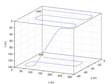
The trajectory described by the vehicle is shown in Fig. 2.

Figure 2: Trajectory described by the vehicle

Sensor noise was considered for all sensors. In particular, the range, acceleration, and angular velocity measurements are assumed to be corrupted by additive uncorrelated zero-mean white Gaussian noise, with standard deviations of $1\,\rm{m}$, $2\times 10^{-3}\,\rm{m/s^{2}}$, and $0.05$ °/s, respectively. The attitude, parameterized by roll, pitch, and yaw Euler angles, was also assumed to be corrupted by zero-mean additive white Gaussian noise, with standard deviation of $0.03$° for the roll and pitch and $0.3$° for the yaw.

The LBL configuration is composed of 4 acoustic transponders and their positions are

$${\mathbf{s}}_{1}=\left[\begin{array}[]{c}0\\ 0\\ 1000\end{array}\right]\rm{(m)},\;{\mathbf{s}}_{2}=\left[\begin{array}[]{c}1000\\ 0\\ 1000\end{array}\right]\rm{(m)},$$

$${\mathbf{s}}_{3}=\left[\begin{array}[]{c}0\\ 1000\\ 1000\end{array}\right]\rm{(m)},\;{\mathbf{s}}_{4}=\left[\begin{array}[]{c}0\\ 0\\ 500\end{array}\right]\rm{(m)},$$

which satisfy Assumption 1.

To tune the Kalman filter, the state disturbance intensity matrix was chosen as ${\mathbf{Q}}_{x}=10^{-5}{\mathbf{I}}$ and the output noise intensity matrix as ${\mathbf{Q}}_{y}=\rm{diag}\left(1,1,1,1,2,2,2,2,2,2\right)$. The initial conditions were set to zero for the position and velocity. The acceleration of gravity was initialized closed to the true value, with $\left[0\;0\;10\right]^{T}\rm{m/s^{2}}$ as the attitude is measured and the magnitude of the acceleration of gravity is usually known. Notice that it would be possible to initialize the position with a close estimate obtained from the inversion of the first set of LBL range measurements. The states corresponding to the range measurements were initialized with the first set of measurements while the remaining states were set to zero, apart from $x_{11}$, which corresponds to the square of the magnitude of the acceleration of gravity, which was initialized with 100.

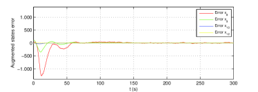
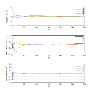
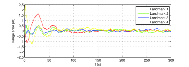
The initial evolution of the position, velocity, and acceleration of gravity errors is depicted in Fig. 3, whereas the initial evolution of the range errors is shown in Fig. 4. The initial convergence of the remaining state errors is shown in Fig. 5. As it can be seen from the various plots, the convergence rate of the filter is quite fast.

Figure 3: Initial convergence of the position, velocity, and acceleration of gravity error

Figure 4: Initial convergence of the range errors

Figure 5: Initial convergence of the error of the augmented states $x_{8}$, $x_{9}$, $x_{10}$, and $x_{11}$

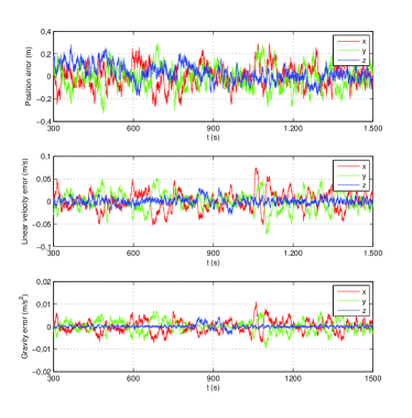
In order to better illustrate the performance achieved with the proposed solution, the steady-state errors of the position, velocity, and acceleration of gravity are shown in Fig. 6. Notice that the errors are confined to very tight intervals, in spite of the realistic measurement noise.

Figure 6: Detailed evolution of the position, velocity, and acceleration of gravity error

The proposed filter was compared against two different solutions: the first is the well-known Extended Kalman Filter; the second consists in applying the linear Kalman filter proposed in Batista et al. (2009b) using a position algebraic estimate obtained from the range measurements to feed the filter. Unfortunately, it is not possible to show the results here due to the lack of space, but in short, the performance of the proposed solution is similar to the EKF and outperforms the one based on the algebraic inversion of the problem. These results will be shown in an extended version of the paper.

5 Conclusions

This paper presented a novel Long Baseline (LBL) position and velocity navigation filter for underwater vehicles based directly on the sensor measurements. Traditional solutions resort either to the Extended Kalman Filter (EKF) or to solutions based on position algebraic estimates obtained from the range measurements. The solution presented in the paper departs from previous approaches as the range measurements are explicitly embedded in the filter design, therefore avoiding inversion algorithms. Moreover, the nonlinear system dynamics are considered to their full extent and no linearizations are carried out whatsoever, which allows to show that the filter error dynamics are globally asymptotically stable. State augmentation is at the core of the proposed framework. Indeed, the proposed filter has $13+n_{\scriptscriptstyle L}$ states, which compares to a minimum of 9 states for traditional solutions. It is the opinion of the authors that the achieved performance coupled with the guarantee of global asymptotic stability justify the additional computational complexity, at least for those missions where extreme constraints on power do not exist.

Under simulation environment it was shown that the filter achieves similar performance to the Extended Kalman Filter (EKF) and outperforms linear position and velocity filters based on position algebraic estimates obtained directly from the range measurements. The advantage over the EKF is however clear due to the GAS property of the proposed solution, which is not guaranteed for the EKF.

Finally, although sensor bias, in particular, accelerometer bias, is a very important problem, in this paper it is assumed, for the sake of clarity of presentation and simplicity of design, that the accelerometer has been previously calibrated. Nevertheless, it is easy to include the accelerometer bias in the system design, which leads to observability conditions so that it is possible to estimate both the gravity and the bias, according to previous work by the authors. The overall system design and observability analysis will be presented elsewhere.

References

• Alcocer et al. (2007) Alcocer, A., Oliveira, P., and Pascoal, A. (2007). Study and Implementation of an EKF GIB-based Underwater Positioning System. Control Engineering Practice,, 15(6), 689–701.
• Batista et al. (2008) Batista, P., Silvestre, C., and Oliveira, P. (2008). Position and Velocity Navigation Filters for Marine Vehicles. In Proceedings of the 17th IFAC World Congress, 15016–15021. Seoul, Korea.
• Batista et al. (2009a) Batista, P., Silvestre, C., and Oliveira, P. (2009a). Necessary and sufficient conditions for the observability of linear motion quantities in strapdown navigation systems. In Proceedings of the 2009 American Control Conference, 1177–1182. Saint Louis, USA.
• Batista et al. (2009b) Batista, P., Silvestre, C., and Oliveira, P. (2009b). Position and Velocity Optimal Sensor-based Navigation Filters for UAVs. In Proceedings of the 2009 American Control Conference, 5404–5409. Saint Louis, USA.
• Batista et al. (2009c) Batista, P., Silvestre, C., and Oliveira, P. (2009c). Single Range Navigation in the presence of Constant Unknown Drifts. In Proceedings of the 2009 European Control Conference, 3983–3988. Budapest, Hungary.
• Batista et al. (2010) Batista, P., Silvestre, C., and Oliveira, P. (2010). Single Beacon Navigation: Observability Analysis and Filter Design. In Proc. 2010 American Control Conference (accepted). Baltimore, USA.
• Brockett (1970) Brockett, R.W. (1970). Finite Dimensional Linear Systems. Wiley.
• Hermann and Krener (1977) Hermann, R. and Krener, A. (1977). Nonlinear controllability and observability. IEEE Transactions on Automatic Control, 22(5), 728–740.
• Jouffroy and Opderbecke (2004) Jouffroy, J. and Opderbecke, J. (2004). Underwater vehicle trajectory estimation using contracting PDE-based observers. In Proceedings of the 2004 American Control Conference, volume 5, 4108–4113. Boston, MA, USA.
• Kelly (1994) Kelly, A. (1994). Modern Inertial and Satellite Navigation Systems. Technical Report CMU-RI-TR-94-15, Robotics Institute, Carnegie Mellon University, Pittsburgh, PA.
• Kinsey et al. (2006) Kinsey, J., Eustice, R., and Whitcomb, L. (2006). A Survey of Underwater Vehicle Navigation: Recent Advances and New Challenges. In Proceedings of the 7th IFAC Conference on Manoeuvring and Control of Marine Craft. Lisboa, Portugal.
• Kinsey and Whitcomb (2003) Kinsey, J. and Whitcomb, L. (2003). Preliminary field experience with the DVLNAV integrated navigation system for manned and unmanned submersibles. In Proceedings of the 1st IFAC workshop on guidance and control of underwater vehicles, 83–88. Newport, South Wales, UK.
• Larsen (2000) Larsen, M. (2000). Synthetic long baseline navigation of underwater vehicles. In Proceedings of the 2000 MTS/IEEE Oceans, volume 3, 2043–2050. Providence, RI, USA.
• Larsen (2001) Larsen, M. (2001). Autonomous navigation of underwater vehicles. Ph.d. dissertation, Department of Automation, Technical University of Denmark.
• Leonard et al. (1998) Leonard, J., Bennett, A., Smith, C., and Feder, H. (1998). Autonomous underwater vehicle navigation. Technical Report Technical Memorandum 98-1, MIT Marine Robotics Laboratory.
• Sukkarieh et al. (1999) Sukkarieh, S., Nebot, E., and Durrant-Whyte, H. (1999). A high integrity IMU/GPS navigation loop for autonomous land vehicle applications. IEEE Transactions on Robotics and Automation, 15(3), 572–578.
• Thomas (1998) Thomas, H. (1998). GIB buoys: an interface between space and depths of the oceans. In Proceedings of the 1998 Workshop on Autonomous Underwater Vehicles,, 181–184. Cambridge, MA, USA.
• Vaganay et al. (1998) Vaganay, J., Bellingham, J., and Leonard, J. (1998). Comparison of fix computation and filtering for autonomous acoustic navigation. International Journal of Systems Science, 29(10), 1111–1122.
• Vik, B. and Fossen, T. (2001) Vik, B. and Fossen, T. (2001). A nonlinear observer for GPS and INS integration. In Proceedings of the 40th IEEE Conference on Decision and Control, volume 3, 2956–2961. Orlando, Florida, USA.
• Youngberg (1992) Youngberg, J. (1992). Method for extending gps to underwater applications.
• Yun et al. (1999) Yun, X., Bachmann, E., McGhee, R., Whalen, R., Roberts, R., Knapp, R., Healey, A., and Zyda, M. (1999). Testing and evaluation of an integrated gps/ins system for small auv navigation. IEEE Journal of Oceanic Engineering, 24(3), 396–404.