Constraining the unexplored period between reionization and the dark ages with observations of the global 21 cm signal
Abstract
Observations of the frequency dependence of the global brightness temperature of the redshifted 21 cm line of neutral hydrogen may be possible with single dipole experiments. In this paper, we develop a Fisher matrix formalism for calculating the sensitivity of such instruments to the 21 cm signal from reionization and the dark ages. We show that rapid reionization histories with duration can be constrained, provided that local foregrounds can be well modelled by low order polynomials. It is then shown that observations in the range can feasibly constrain the Ly and X-ray emissivity of the first stars forming at , provided that systematic temperature residuals can be controlled to less than 1 mK. Finally, we demonstrate the difficulty of detecting the 21 cm signal from the dark ages before star formation.
I Introduction
The transition of the Universe from the dark ages following hydrogen recombination through to the epoch of reionization remains one of the least constrained frontiers of modern cosmology. Observing the sources responsible for heating and ionizing the intergalactic medium (IGM) at redshifts pushes current observational techniques to the limit. Plans are underway to construct low-frequency radio telescopes, such as LOFAR111http://www.lofar.org/, MWA222http://www.MWAtelescope.org/, PAPER333Parsons et al. (2010), and SKA444http://www.skatelescope.org/, to observe the red-shifted 21 cm line of neutral hydrogen. These experiments aim to map the state of the intergalactic medium via tomographic observations of 3D fluctuations in the 21 cm brightness temperature. A simpler and significantly lower cost alternative to this would be measurements of the global 21 cm signal integrated over the sky Madau et al. (1997); Shaver et al. (1999); Sethi (2005), which can be achieved by single dipole experiments like EDGES Bowman et al. (2008) or CoRE Chippendale et al. (2005). Although such experiments are today in their infancy, their potential is large. In this paper, we explore the potential for these global sky experiments to measure the 21 cm signal and constrain the high redshift Universe.
We may draw a historical analogy with the Cosmic Background Explorer (COBE), whose FIRAS instrument measured the blackbody spectrum of the cosmic microwave background (CMB) Mather et al. (1994) while the DMR instrument measured the level of temperature fluctuations Smoot et al. (1992). The precise measurement of a blackbody spectrum placed tight constraints on early energy injection, since no Compton- or -distortion were seen, and provided important evidence confirming the big bang paradigm. The detection of angular fluctuations paved the way for more sensitive experiments such as BOOMERANG Lange et al. (2001) and WMAP Spergel et al. (2003), which provided precision measurements of the CMB acoustic peaks. While, at the moment, attention is focussed on experiments designed to measure 21 cm fluctuations, it is important not to neglect the possibility of measuring the global signal.
The evolution of the 21 cm signal is driven primarily by the amount of neutral hydrogen and the coupling between the 21 cm spin temperature and the gas temperature. It is able to act as a sensitive thermometer when the IGM gas temperature is less than the CMB temperature placing constraints on energy injection that leads to heating. For example, the first black holes to form generate X-rays, which heat the gas. More exotic processes such as annihilating dark matter might have also been important. Additionally, energy injection in the form of Ly production modifies the strength of the coupling. This provides a way of tracking star formation, which will be the dominant source of Ly photons. As we show, the spectral structure of the 21 cm signal is much richer than that of a blackbody so that many things can be learnt about the early Universe. Given the uncertainties, we develop a model approach based upon those physical features most likely to be present.
The single most important factor determining the sensitivity of dipoles to astrophysics will be their ability to remove galactic foregrounds (e.g. Oh and Mack, 2003; Di Matteo et al., 2004). Exploitation of spectral smoothness to remove foregrounds by fitting low order polynomials is key to avoiding throwing the signal away with the foreground. To quantify this, we develop a simple Fisher matrix formalism and validate it against more detailed numerical parameter fitting. This provides us with a way of quantitatively addressing the ability of global 21 cm experiments to constrain reionization and the astrophysics of the first galaxies Loeb (2010). Similar work on the subject Sethi (2005) ignored the influence of foregrounds limiting its utility considerably.
Much of the power of this technique stems from the limitations of other observational probes. While next generation telescopes such as JWST555http://www.jwst.nasa.gov/, GMT666http://www.gmto.org/, EELT777http://www.eso.org/sci/facilities/eelt/ or TMT888http://www.tmt.org/ may provide a glimpse of the Universe at they peer through a narrow field of view and are unlikely to touch upon redshifts . As we will show, 21 cm global experiments could potentially provide crude constraints on even higher redshifts at a much lower cost.
The structure of this paper is as follows. In §II, we begin by describing the basic physics that drives the evolution of the 21 cm global signature and drawing attention to the key observable features. We follow this in §III with a discussion of the foregrounds, which leads into our presenting a Fisher matrix formalism for predicting observational constraints in §IV. In §V and §VI we apply this formalism to the signal from reionization and the first stars, respectively. After a brief discussion in §VII of the prospects for detecting the signal from the dark ages before star formation, we conclude in §VIII.
Throughout this paper where cosmological parameters are required we use the standard set of values , , , (with ), , and , consistent with the latest measurements (Komatsu et al., 2009).
II Physics of the 21 cm global signal
The physics of the cosmological 21 cm signal has been described in detail by a number of authors (Furlanetto et al., 2006a; Pritchard and Loeb, 2008) and we focus here on those features relevant for the global signal. It is important before we start to emphasise our uncertainty in the sources of radiation in the early Universe, so that we must of necessity extrapolate far beyond what we know to make predictions for what we may find. Nonetheless the basic atomic physics is well understood and a plausible understanding of the likely history is possible.
The 21 cm line frequency redshifts for into the range 200-50 MHz. The signal strength may be expressed as a differential brightness temperature relative to the CMB
| (1) |
where is the hydrogen neutral fraction, is the overdensity in baryons, is the 21 cm spin temperature, is the CMB temperature, is the Hubble parameter, and the last term describes the effect of peculiar velocities with the derivative of the velocities along the line of sight. Throughout this paper, we will neglect fluctuations in the signal so that neither of the terms nor the peculiar velocities will be relevant. Fluctuations in and will be relevant for the details of the signal, but are not required to get the broad features of the signal, on which we focus here.
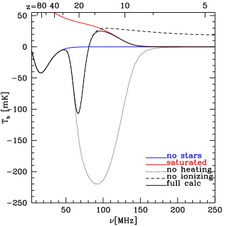
The evolution of is thus driven by the evolution of and and is illustrated for redshifts in Figure 1. Early on, collisions drive to the gas temperature , which after thermal decoupling (at ) has been cooling faster than the CMB leading to a 21 cm absorption feature (). Collisions start to become ineffective at redshifts and scattering of CMB photons begins to drive causing the signal to disappear. In the absence of star formation, this would be the whole story Loeb and Zaldarriaga (2004).
Star formation leads to the production of Ly photons, which resonantly scatter off hydrogen coupling to via the Wouthysen-Field effect Wouthuysen (1952); Field (1958). This produces a sharp absorption feature beginning at . If star formation also generates X-rays they will heat the gas, first causing a decrease in as the gas temperature is heated towards and then leading to an emission signal, as the gas is heated to temperatures . For all dependence on the spin temperature drops out of equation (1) and the signal becomes saturated. This represents a hard upper limit on the signal. Finally reionization will occur as UV photons produce bubbles of ionized hydrogen that percolate, removing the 21 cm signal.
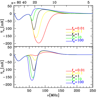
We may thus identify five main events in the history of the 21 cm signal: (i) collisional coupling becoming ineffective (ii) Ly coupling becoming effective (iii) heating occurring (iv) reionization beginning (v) reionization ending. In the scenario described above the first four of these events generates a turning point () and the final event marks the end of the signal. We reiterate that the astrophysics of the sources driving these events is very uncertain, so that when or even if these events occur as described is currently unknown. Figure 2 shows a set of histories for different values of the X-ray and Ly emissivity, parametrized about our fiducial model by and representing the product of the emissivity and the star formation efficiency following Ref. Pritchard and Loeb (2008). Clearly the positions of these features may move around both in the amplitude of and the frequency at which they occur.
We view this to be the most likely sequence of events for plausible astrophysical models. We are reassured in this sequencing since, in the absence of Ly photons escaping from galaxies Higgins and Meiksin (2009), X-rays will also produce Ly photons Chen and Miralda-Escudé (2008); Chuzhoy et al. (2006) and so couple to and, in the absence of X-rays, scattering of Ly photons heats the gas Ciardi and Madau (2003). In each case the relative sequence of events is likely to be maintained. We will return to how different models may be distinguished later and now turn to the presence of foregrounds between us and the signal.
III Foregrounds
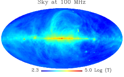
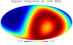
At the frequencies of interest (10-250 MHz), the sky is dominated by synchrotron emission from the galaxy. A useful model of the sky has been put together by Ref. (de Oliveira-Costa et al., 2008) using all existing observations. The sky at 100 MHz is shown in Figure 3, where the form of the galaxy is clearly visible. In this paper, we will be focusing upon observations by single dipole experiments. These have beam shapes with a typical field-of-view of tens of degrees. The lower panel of Figure 3 shows the beam of dipole (approximated here as a single lobe) sitting at the MWA site in Australia (approximate latitude 26∘59’S), observing at zenith, and integrated over a full day. Although the dipole does not see the whole sky at once it does average over large patches. We will therefore neglect spatial variations (although we will return to this point in our conclusions).
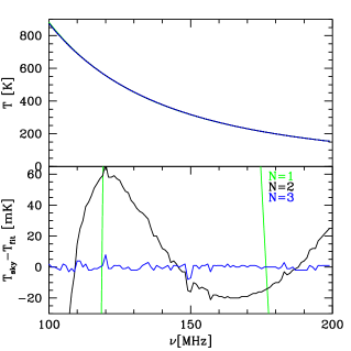
Averaging the foregrounds over the dipole’s angular response gives the spectrum shown in the top panel of Figure 4. First note that the amplitude of the foregrounds is large compared to the 10 mK signal. Nonetheless, given the smooth frequency dependence of the foregrounds we are motivated to try fitting the foreground out using a low order polynomial in the hope that this leaves the signal behind. This has been shown by many authors (e.g. McQuinn et al., 2006; Wang and Hu, 2006) to be a reasonable procedure in the case of 21 cm tomography. There the inhomogeneities fluctuate rapidly with frequency, so that only the largest Fourier modes of the signal are removed. In the case of the global 21 cm signal our signal is relatively smooth in frequency, especially if the bandwidth of the instrument is small. Throwing the signal out with the foregrounds is therefore a definite concern.
Throughout this paper, we will fit the foregrounds using a polynomial of the form
| (2) |
Here is a pivot scale and we will generally recast to emphasise that the zeroth order coefficient more naturally has units of temperature. The lower panel of Figure 4 shows the residuals left over after fitting and subtracting polynomials of different order to the foregrounds. It is apparent that a polynomial of at least is necessary to remove the foreground. Unfortunately, our current knowledge of the low frequency sky is not sufficient for us to conclusively say that we will not need a higher order polynomial or to accurately quantify the minimum level of residuals that will be left on fitting the signal. The residuals visible in Figure 4 for are dominated by numerical limitations of the sky model being used and have averaged over the band.

Figure 5 shows the evolution of the best fit values as we change the order of the fit. The first four values are non-zero and therefore important to the fit. The next two hover around zero (although as the order increases they move away from zero). This supports the inference that only the first four parameters are necessary and after that we are beginning to over fit. We therefore take as our fiducial model for the foreground the form
| (3) |
with parameter values , , , , , chosen from fitting to the band MHz. These values are roughly consistent with those found by the observations reported in Ref. Rogers and Bowman (2008), which found and over the same band. Where necessary we include additional terms as for . Fitting to a different bandwidth and pivot frequency will modify these values. For example, fitting to MHz with MHz yields, , , , . Aside from the overall normalisation, there is little qualitative change in the shape.
IV Fisher calculation
The main objective of this paper is to develop a formalism for quantifying the ability of global 21 cm experiments to constrain astrophysical parameters. A straightforward, but brute force approach, is to model the signal, add a foreground, and then use Monte-Carlo (MC) fitting techniques to see how well model parameters may be constrained. When faced with the large space of model parameters to be explored this is inadequate. We therefore explore the use of the Fisher matrix approach, applicable if the model likelihood is well approximated by a multivariate Gaussian. We will later show that this is a good approximation by testing it directly against the results of direct MC fitting.
The Fisher matrix takes the form Eisenstein et al. (1999)
| (4) |
where is the covariance matrix and . For the 21 cm global signature, our observable is the antennae temperature , where we assume the dipole sees the full sky so that spatial variation can be ignored. We divide the signal into frequency bins {} of bandwidth running between [, ]. The covariance matrix is taken to be diagonal, since errors in different frequency bins are expected to be uncorrelated, so that it is given by
| (5) |
with the thermal noise given by the radiometer equation
| (6) |
assuming an integration time . In this paper, we will consider single dipole experiments, but the noise could be further reduced by a factor through the incoherent summing of the signal from multiple dipoles. Finally, we can allow for a limiting floor in the noise due to foreground fitting residuals or instrumental noise by setting .
Under these assumptions the Fisher matrix takes the form
| (7) |
where the parameter set includes both foreground and signal model parameters. Here the first term is the information contained in the amplitude of the noise and is subdominant for reasonable experiments ((cf. Sethi, 2005)). Given this Fisher matrix, the best parameter constraints achievable on parameter are given by the Cramer-Rao inequality . This Fisher matrix offers a fast and, as we will show in the next section, reliable means of calculating the expected constraints for 21 cm global experiments.
The assumption of a full sky observation is not strictly valid, since the dipole sees the sky with a beam tens of degrees across. Both foreground and signal will show spatial variation. Fluctuations in the 21 cm signal can be large in amplitude, but span a characteristic scale of order a few arcminutes corresponding to the size of the ionized bubbles. As such our beam will average over many of these, so that we do not expect significant spatial fluctuations to survive. The foregrounds are another matter and spatial variation may be a mixed blessing. In practice, each foreground parameters should be fitted independently in each pixel. Since the signal is common to all pixels, exploiting the spatial variation of the foregrounds could be used to remove them more efficiently.
So far, we have assumed that the instrument’s frequency response can be calibrated out perfectly. At present one of the limiting factors of the EDGES experiment is that the dipole’s frequency response is uncalibrated. This has the effect of convolving both foregrounds and signal with some unknown function of frequency. Provided that this function is smooth the main complication so introduced is that the convolved foregrounds are no longer easily described by a low order polynomial. In Ref. Bowman et al. (2008), a 12th order polynomial in was used for the foreground fitting, primarily in order to fit out the instrumental response. Since this is very much a prototype experiment, we will optimistically assume that this instrumental problem can be dealt with in more advanced designs.
V Reionization
Next, we will consider the possibility of constraining the evolution of the hydrogen neutral fraction from the global 21 cm signal. Predicting the reionization history has attracted a great deal of attention in recent years Loeb (2010). Constraints arise from the Ly forest, the optical depth to the CMB, and numerous other locations. Although these may be combined to constrain the reionization history (e.g. Pritchard et al., 2009), the quality of current constraints is poor. In general though, reionization is expected to be a relatively extended process.
Given the uncertainty associated with making detailed predictions for the evolution of , we adopt as a toy model for reionization a tanh step (as used by the WMAP7 analysis Larson et al. (2010)) with parameters describing the two main features of reionization: its mid point and duration . We will further assume that the 21 cm spin temperature is saturated at the relevant redshifts (a reasonable although not guaranteed simplifying assumption Ciardi and Madau (2003); Pritchard and Furlanetto (2007)). Under these assumptions, the 21 cm brightness temperature is given by
| (8) |
In principle, the amplitude of the signal is calculable from first principles ( for our fiducial cosmology), but we leave it as a free parameter. This helps us gauge how well the experiment is really detecting the 21 cm signal. Figure 6 shows a few different histories for this model.

Before exploring the detection space for 21 cm experiments, we validate our Fisher matrix against a more numerically intensive Monte-Carlo. We consider an experiment covering the frequency range in 50 bins and integrating for 500 hours (these parameters mimic EDGES with an order of magnitude longer integration time). Taking fiducial values of , , and , we fit the model and foreground for realisations of the thermal noise. This yields an estimate of the parameter uncertainty that can be expected from observations and can be used to test our Fisher matrix calculation. The resulting parameter contours are shown in Figure 7 along with the Fisher matrix constraints. That they are in good agreement validates our underlying formalism.
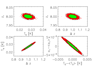
The error ellipses show that there is a strong degeneracy between and . This is a consequence of the way in which foreground fitting removes power from more extended histories making it difficult to distinguish a larger amplitude extended scenario from a lower amplitude sharper scenario.
Despite the good agreement, this formalism breaks down when the Fisher matrix errors become large enough that reionization parameters are not well constrained. Although this is not a major hurdle here, caution should be used when errors are much larger than the parameters being constrained.
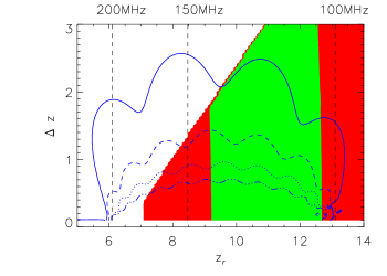
The resulting potential detection region for the above experiment is shown in Figure 8, where we consider several different orders of polynomial fit. The detection region shows a number of wiggles associated with points in the frequency range where the shape of the 21 cm signal becomes more or less degenerate with the polynomial fitting. We also show the 1- and constraint regions from WMAP’s optical depth measurement. These constrain the redshift of reionization, but say little about how long it takes. Adding in a prior based upon Ly forest observations that the Universe is fully ionized by (specified here as ) removes the region of parameter space with large and low .
Global experiments can take a good sized bite out of the remaining parameter space. They are sensitive to the full range of redshifts, but primarily to the sharpest reionization histories. Only if can histories with be constrained and histories with appear too extended for high significance detections.
This is unfortunate, since Pritchard et al. (2009) found that most reionization histories compatible with the existing data have , suggesting it will be difficult for global experiments to probe the most likely models. An important caveat to these conclusions is that the tanh model that we have used here is a toy model of reionization. More realistic models may have more detectable features since they often end rapidly, but have a long tail to high redshifts.
VI First sources
We now turn from reionization to the signal produced by the first galaxies, which generate an early background of Ly and X-ray photons. This region is essentially unconstrained by existing observations and global 21 cm experiments represent one of the only upcoming ways of probing this epoch.
Although models for the signal during this epoch exist (Furlanetto, 2006; Pritchard and Loeb, 2008), it will be useful to focus on physical features of the signal that are both observable and model independent. With this in mind, we parametrize the signal in terms of the turning points of the 21 cm signal. Figure 9 shows the evolution of and its frequency derivative. As discussed in §II, there are four turning points associated with: (0) a minimum during the dark ages where collisional coupling begins to become ineffective, (1) a maximum at the transition from the dark ages to the Ly pumping regime as Ly pumping begins to be effective, (2) an absorption minimum as X-ray heating begins to raise the signal towards emission, (3) an emission maximum as the signal becomes saturated and starts to decrease with the cosmic expansion. Finally reionization completes providing a fifth point. Asymptotically the signal goes to zero at very low and high frequencies.
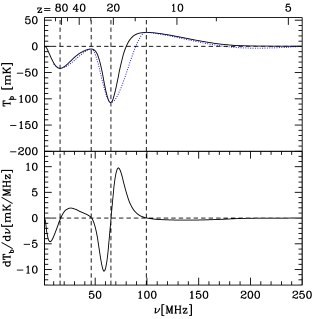
In order to have a simple model for the evolution of the signal, we adopt parameters , , , , and for the frequency and amplitude of the turning points and the frequency at the end of reionization. For clarity of notation we will label these points as (with ). We then model the signal with a simple cubic spline between these points with the additional condition that the derivative should be zero at the turning points (enforced by doubling the data points at the turning points and offsetting them by ).
For our fiducial model, we adopt the fiducial parameter set of Ref. (Pritchard and Loeb, 2008), assuming a star forming efficiency , a Ly emissivity expected for Population II stars , and X-ray emissivity appropriate for extrapolating the locally observed X-ray-FIR correlation, . This gives turning points =(16.1 MHz, -42 mK), =(46.2 MHz, -5 mK), =(65.3 MHz, -107 mK), =(99.4 MHz, 27 mK), and =(180 MHz, 0 mK). The resulting spline fit is shown in the top panel of Figure 9. The model does a good job of capturing the general features of the 21 cm signal, although there are clear differences in the detailed shape. Since global experiments are unlikely to constrain more than the sharpest features, this approach should be adequate for our purposes.
There is considerable uncertainty in the parameters of this model, and so to gauge the likely model dependence of the turning points, we make use of the model of Ref. (Pritchard and Loeb, 2008). Varying the Ly , X-ray, and UV emissivity by two orders of magnitude on either side of their fiducial values we find the position and amplitude of the turning points to give the parameter space shown in Figure 10. This provides a useful guide to targeting observations in frequency space. We have found that a global experiment has very little sensitivity to features lying outside of the observed frequency band.
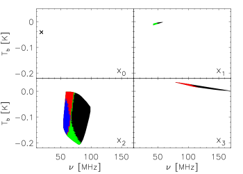
Since we fix the cosmology, appears as a single point. The locations of and are controlled by the Ly and X-ray emissivity respectively. Only shows significant dependence on both Ly and X-ray emissivity leading to a large uncertainty in its position. This is good news observationally, since even a poor measurement of the position of is likely to rule out a wide region of parameter space. Since is the feature with both the largest amplitude and sharpest shape, we expect that this is the best target for observation and makes experiments covering of great interest.
Since our model is approximate, it is important to check whether it leads to significantly biased constraints on the features of interest. One could imagine that fitting the splined shape might lead to biased estimates of the position of the turning points, for example. We have checked this through Monte-Carlo simulation by fitting the turning-point model to the full calculation signal for realisations of the thermal noise. As seen in Figure 11 for an experiment covering 45-145 MHz in 50 bins and integrating for 500 hours, the MC calculation shows no sign of significant biasing and is in good agreement with the Fisher matrix calculation using the turning-point model.
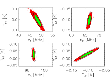
The final panel of Figure 11 shows a degeneracy between and . This might be expected for an experiment whose sensitivity is primarily to the derivative of the signal, which is left unchanged by shifting both of these points up or down.
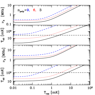
As we examine lower frequencies where the foregrounds are brighter, we must increasingly worry about foreground removal leaving behind systematic residuals that limit the sensitivity of the experiment. In Figure 12, we plot the sensitivity of the same experiment to as a function of this residual floor for different values of . Polynomials with are required to have any chance of detecting the signal. Sensitivity to the signal begins to degrade once becomes greater than 0.1 mK corresponding roughly to the thermal noise for this experiment. A detection of is still possible until .
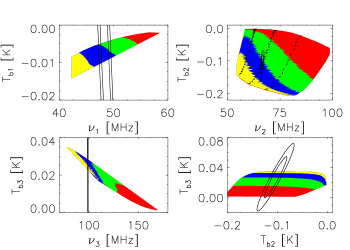
We finish this section by comparing the Fisher matrix constraints from Figure 11 on top of the region spanned by the turning points in Figure 10. This is shown in Figure 13 and gives a sense of the large space of astrophysical models that may be ruled out with a single global experiment. While the experiment has trouble constraining and with any significance, it places relatively good constraints on .
Throughout this section we have chosen to model the 21 cm global signal by a simple cubic spline based upon the turning points of the signal. While this model is simple, one can imagine alternative approaches. Since the experiments are primarily sensitive to the derivative of the 21 cm signal, we might imagine taking the positions of the extrema of the derivative as our parameters and seek to constrain those. We leave the exploration of alternatives such as this to future work.
VII Dark Ages
The physics of the period before star formation at is determined by well known atomic processes and so has much in common with the CMB. However, many models have been put forward that would modify this simple picture with exotic energy deposition via annihilating or decaying dark matter Furlanetto et al. (2006b) or evaporating black holes Mack and Wesley (2008), for example. During the dark ages, the 21 cm signal acts as a sensitive thermometer, potentially capable of constraining these exotic processes. Here we will focus on the standard history and leave consideration of the possibility of detecting other scenarios to future work.
The signal during the dark ages reaches a maximum at , , somewhat larger in amplitude than the reionization emission signal. However, at these low frequencies the foregrounds are extremely large, at , making detection very difficult. Its is worth noting however that global experiments have an advantage over tomographic measurements here, since at these early times structures have had little chance to grow, making the fluctuations much smaller than during reionization. Further, it is easier to imagine launching a single dipole experiment beyond the Earth’s ionosphere rather than the many km2 of collecting area needed for interferometers to probe this epoch Gordon and Pritchard (2009); Jester and Falcke (2009).
Given the large foregrounds, long integration times or many dipoles are required to reach the desired sensitivity level. Taking at a single dipole would need to integrate for to reach 4 mK sensitivity. Removing the foregrounds over this dynamic range without leaving considerable residuals will clearly require very precise instrumental calibration. Given the challenges, we look at the most optimistic case as a limit of what could be accomplished.
Taking an experiment covering in 50 channels and integrating for 8000 hours, we assume a minimal polynomial fit leaving no residuals. The resulting constraint on the position and amplitude of the dark ages feature are shown in Figure 14. Such an experiment is capable of detecting the signal, but only barely. For comparison, we have plotted the uncertainty arising from cosmological measurements of and , the two main parameters determining the 21 cm signal. This uncertainty is much less than the experimental uncertainty.
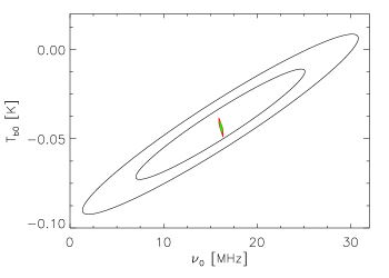
Although we have shown that detecting the dark ages feature from the standard history would be extremely challenging, modified histories arising from exotic energy injection may lead to larger features more easily detected. Since there is no other probe of physics at global 21 cm experiments offer a unique if extremely challenging probe of this period.
VIII Conclusions
Observations of the redshifted 21 cm line potentially provide a new window into the high redshift Universe. Detecting this signal in the presence of large foregrounds is challenging and it is important to explore all avenues for exploiting the signal. In this paper, we have focussed upon the possibility of using single dipole experiments to observe the all-sky 21 cm signal, in contrast to the 21 cm fluctuations targeted by MWA, LOFAR, PAPER, and SKA. Experiments targeting this global signal are in their infancy. We emphasise that instruments built from a few dipoles targeting the global 21 cm signal can be several orders of magnitude cheaper to build than interferometers targeting the fluctuations. Their scientific return will be similarly less, but at this stage where we know so little about the first sources, even that little is extremely valuable.
As we have outlined in this paper, the 21 cm signal generated by astrophysical processes has a well defined form, although the input parameters are only poorly understood. We have demonstrated that, at the level of our current knowledge, describing the Galactic foregrounds requires at least a 3rd order polynomial. At this level, we are able to remove the foregrounds to the sub-mK level, although in practice this procedure may be more complicated. In order to characterise the sensitivity of these experiments to the signal, we developed a Fisher matrix formalism and validated it against more numerical fitting of the model parameters. This Fisher matrix approach allows rapid calculations of the experimental sensitivity and appears to reproduce more detailed calculations very well.
Having developed this formalism we applied it to the signal from reionization and the epoch of the first stars. Using a toy model of reionization, we demonstrated that EDGES-like experiments should be capable of constraining rapid reionization histories with . More promisingly, these experiments can rule out a wide variety of astrophysical models for the signal from the first stars where the evolution of the spin temperature is important. We used a straightforward fitting form for the signal based upon the positions of the turning points and showed that these features could be constrained, with the deepest absorption trough providing the best observational target.
Finally, we briefly explored the possibility of detecting the absorption feature present before star formation began. The increased foreground brightness at low frequencies make it very difficult to constrain this feature and will require long integration times and more sophisticated methods of foreground removal.
This paper represents a first serious look at the prospects for using global measurements of the 21 cm signal to constrain astrophysics. As a result, there are a number of places where future work might improve upon our calculations. These include investigating the effects of finite sky coverage, incorporating an arbitrary instrumental frequency response, and allowing for the removal of frequency channels corrupted by terrestrial radio interference.
Acknowledgements
We would like to thank Judd Bowman and Angelica de Oliveira-Costa for useful conversations. Figure 3 was generated using HEALpix Górski et al. (2005) and the global sky model software of Ref. de Oliveira-Costa et al. (2008). JRP is supported by NASA through Hubble Fellowship grant HST-HF-01211.01-A awarded by the Space Telescope Science Institute, which is operated by the Association of Universities for Research in Astronomy, Inc., for NASA, under contract NAS 5-26555. AL acknowledges funding from NSF grant AST-0907890 and NASA grants NNA09DB30A and NNX08AL43G.
References
- Parsons et al. (2010) A. R. Parsons, D. C. Backer, G. S. Foster, et al., Astron. J. 139, 1468 (2010), eprint arXiv:0904.2334.
- Madau et al. (1997) P. Madau, A. Meiksin, and M. J. Rees, Astrophys. J. 475, 429 (1997).
- Shaver et al. (1999) P. A. Shaver, R. A. Windhorst, P. Madau, and A. G. de Bruyn, Astron. & Astrophys. 345, 380 (1999), eprint arXiv:astro-ph/9901320.
- Sethi (2005) S. K. Sethi, Mon. Not. R. Astron. Soc. 363, 818 (2005), eprint arXiv:astro-ph/0508172.
- Bowman et al. (2008) J. D. Bowman, A. E. E. Rogers, and J. N. Hewitt, Astrophys. J. 676, 1 (2008), eprint arXiv:0710.2541.
- Chippendale et al. (2005) A. P. Chippendale, E. Subrahmanyan, and R. Ekers (2005), presented at New Techniques and Results in Low Frequency Radio Astronomy, Hobart.
- Mather et al. (1994) J. C. Mather et al., Astrophys. J. 420, 439 (1994).
- Smoot et al. (1992) G. F. Smoot et al., Astrophys. J. Lett. 396, L1 (1992).
- Lange et al. (2001) A. E. Lange et al., Phys. Rev. D 63, 042001 (2001), eprint arXiv:astro-ph/0005004.
- Spergel et al. (2003) D. N. Spergel, L. Verde, H. V. Peiris, E. Komatsu, M. R. Nolta, C. L. Bennett, M. Halpern, G. Hinshaw, N. Jarosik, A. Kogut, et al., Astrophys. J. Suppl. Ser. 148, 175 (2003), eprint arXiv:astro-ph/0302209.
- Oh and Mack (2003) S. P. Oh and K. J. Mack, Mon. Not. R. Astron. Soc. 346, 871 (2003), eprint arXiv:astro-ph/0302099.
- Di Matteo et al. (2004) T. Di Matteo, B. Ciardi, and F. Miniati, Mon. Not. R. Astron. Soc. 355, 1053 (2004), eprint arXiv:astro-ph/0402322.
- Loeb (2010) A. Loeb, How did the first stars and galaxies form? (Princeton University Press, 2010).
- Komatsu et al. (2009) E. Komatsu et al., Astrophys. J. Suppl. Ser. 180, 330 (2009), eprint arXiv:0803.0547.
- Furlanetto et al. (2006a) S. R. Furlanetto, S. P. Oh, and F. H. Briggs, Phys. Rept. 433, 181 (2006a), eprint arXiv:astro-ph/0608032.
- Pritchard and Loeb (2008) J. R. Pritchard and A. Loeb, Phys. Rev. D 78, 103511 (2008), eprint arXiv:0802.2102.
- Loeb and Zaldarriaga (2004) A. Loeb and M. Zaldarriaga, Phys. Rev. Lett. 92, 211301 (2004), eprint arXiv:astro-ph/0312134.
- Wouthuysen (1952) S. A. Wouthuysen, Astron. J. 57, 31 (1952).
- Field (1958) G. B. Field, Proc. I. R. E. 46, 240 (1958).
- Higgins and Meiksin (2009) J. Higgins and A. Meiksin, Mon. Not. R. Astron. Soc. 393, 949 (2009), eprint arXiv:0811.1184.
- Chen and Miralda-Escudé (2008) X. Chen and J. Miralda-Escudé, Astrophys. J. 684, 18 (2008), eprint arXiv:astro-ph/0605439.
- Chuzhoy et al. (2006) L. Chuzhoy, M. A. Alvarez, and P. R. Shapiro, Astrophys. J. Lett. 648, L1 (2006), eprint arXiv:astro-ph/0605511.
- Ciardi and Madau (2003) B. Ciardi and P. Madau, Astrophys. J. 596, 1 (2003), eprint arXiv:astro-ph/0303249.
- de Oliveira-Costa et al. (2008) A. de Oliveira-Costa, M. Tegmark, B. M. Gaensler, J. Jonas, T. L. Landecker, and P. Reich, Mon. Not. R. Astron. Soc. 388, 247 (2008), eprint arXiv:0802.1525.
- McQuinn et al. (2006) M. McQuinn, O. Zahn, M. Zaldarriaga, L. Hernquist, and S. R. Furlanetto, Astrophys. J. 653, 815 (2006), eprint arXiv:astro-ph/0512263.
- Wang and Hu (2006) X. Wang and W. Hu, Astrophys. J. 643, 585 (2006), eprint arXiv:astro-ph/0511141.
- Rogers and Bowman (2008) A. E. E. Rogers and J. D. Bowman, Astron. J. 136, 641 (2008), eprint arXiv:0806.2868.
- Eisenstein et al. (1999) D. J. Eisenstein, W. Hu, and M. Tegmark, Astrophys. J. 518, 2 (1999), eprint arXiv:astro-ph/9807130.
- Pritchard et al. (2009) J. R. Pritchard, A. Loeb, and J. S. B. Wyithe, ArXiv e-prints (2009), eprint arXiv:0908.3891.
- Larson et al. (2010) D. Larson, J. Dunkley, G. Hinshaw, E. Komatsu, M. R. Nolta, C. L. Bennett, B. Gold, M. Halpern, R. S. Hill, N. Jarosik, et al., ArXiv e-prints (2010), eprint arXiv:1001.4635.
- Pritchard and Furlanetto (2007) J. R. Pritchard and S. R. Furlanetto, Mon. Not. R. Astron. Soc. 376, 1680 (2007), eprint arXiv:astro-ph/0607234.
- Furlanetto (2006) S. R. Furlanetto, Mon. Not. R. Astron. Soc. 371, 867 (2006), eprint arXiv:astro-ph/0604040.
- Furlanetto et al. (2006b) S. R. Furlanetto, S. P. Oh, and E. Pierpaoli, Phys. Rev. D 74, 103502 (2006b), eprint arXiv:astro-ph/0608385.
- Mack and Wesley (2008) K. J. Mack and D. H. Wesley, ArXiv e-prints 805 (2008), eprint arXiv:0805.1531.
- Gordon and Pritchard (2009) C. Gordon and J. R. Pritchard, Phys. Rev. D 80, 063535 (2009), eprint arXiv:0907.5400.
- Jester and Falcke (2009) S. Jester and H. Falcke, New Astronomy Review 53, 1 (2009), eprint arXiv:0902.0493.
- Górski et al. (2005) K. M. Górski, E. Hivon, A. J. Banday, B. D. Wandelt, F. K. Hansen, M. Reinecke, and M. Bartelmann, Astrophys. J. 622, 759 (2005), eprint arXiv:astro-ph/0409513.