Early appraisal of the fixation probability in directed networks

Abstract

In evolutionary dynamics, the probability that a mutation spreads through the whole population, having arisen in a single individual, is known as the fixation probability. In general, it is not possible to find the fixation probability analytically given the mutant’s fitness and the topological constraints that govern the spread of the mutation, so one resorts to simulations instead. Depending on the topology in use, a great number of evolutionary steps may be needed in each of the simulation events, particularly in those that end with the population containing mutants only. We introduce two techniques to accelerate the determination of the fixation probability. The first one skips all evolutionary steps in which the number of mutants does not change and thereby reduces the number of steps per simulation event considerably. This technique is computationally advantageous for some of the so-called layered networks. The second technique, which is not restricted to layered networks, consists of aborting any simulation event in which the number of mutants has grown beyond a certain threshold value, and counting that event as having led to a total spread of the mutation. For large populations, and regardless of the network’s topology, we demonstrate, both analytically and by means of simulations, that using a threshold of about $100$ mutants leads to an estimate of the fixation probability that deviates in no significant way from that obtained from the full-fledged simulations. We have observed speedups of two orders of magnitude for layered networks with $10\,000$ nodes.

I Introduction

We consider directed networks in which each node is inhabited by a single individual of a population and whose edges represent the possibilities for an individual’s offspring to replace some other individual. Such networks provide the substrate on which the evolution of the population can be studied given the constraints imposed by their structures. In this modality of evolutionary dynamics, known as evolutionary graph dynamics since its introduction in Lieberman et al. (2005), the population evolves in discrete time steps, each of which involves the fitness-based selection of an individual for reproduction and the use of its offspring to replace one of its out-neighbors in the network. The chief quantity one targets in such studies is the probability that a mutation arising at a randomly chosen individual, henceforth called a mutant, of the otherwise homogeneous population eventually spreads through all the population. This probability is known as the fixation probability.

In the last decade, the study of several other phenomena has been approached from a similar perspective of interacting agents. Such phenomena have included differently constrained forms of the dynamics of evolution Moran (1958); Valleriani and Meene (2007), the spread of epidemics through populations Barthélemy et al. (2004), the emergence of cooperation in biological and social systems Santos and Pacheco (2005); Ohtsuki et al. (2006); Taylor et al. (2007); Fu et al. (2009), and various others Grönlund and Holme (2005); Szabó and Fáth (2007); Pugliese and Castellano (2009). In most cases, what the interacting agents do, driven by either competition or the goal of promoting cooperation, is to spread information through the network in order to attempt to influence the states of other agents. In general, network structure is a major player in affecting the global outcome of such interactions, and this holds to the extent that subtle structural changes can have relevant consequences Kim et al. (2002); Lieberman et al. (2005); Guan et al. (2006); Wu et al. (2006); Ohtsuki et al. (2007a, b); Szolnoki and Szabó (2007). The importance of network structure, in fact, is also central in several other areas, as for example those discussed in Bornholdt and Schuster (2003); Boccaletti et al. (2006); Newman et al. (2006).

The fixation probability is very heavily influenced by the structure of the underlying network as well. In rare cases it is possible to calculate it analytically from both structure and the relative fitnesses of the individuals Lieberman et al. (2005); Antal et al. (2006); Broom and Rychtář (2008); Sood et al. (2008); Masuda and Ohtsuki (2009), but in general one has to resort to simulations of the evolutionary steps. Given the network and the mutant’s fitness, the simulation is conducted as a number of independent events, each of which starts by placing the mutant at a randomly chosen node and then carries out the evolutionary steps until either fixation (all nodes contain mutants) or extinction (no node contains a mutant) occurs. The fraction of events ending in fixation is an estimate of the fixation probability. This simulation-based approach to obtaining the fixation probability can be very time-consuming, not only because many independent events are needed, but also because each event can require a significantly large number of steps to converge. This is illustrated in Fig. 1, which suggests two properties of the simulation process. The first is that events ending in extinction usually require substantially fewer steps to conclude than those ending in fixation. The second is that the number of steps required for fixation varies widely with network topology.

Figure 1: (Color online) Probability densities associated with the number of steps required for extinction and fixation of a mutant $10\%$ fitter than the remainder of the population. Data are log-binned to the base $1.5$ and represent averages over $10^{6}$ events for the $K$-funnel, $10^{7}$ events for the random networks ($10^{4}$ events for each of $10^{3}$ graphs; in the case of the random network with a Poisson-distributed number of out-neighbors, each of these graphs has at least $95\%$ of the nodes in the GSCC). Arrows indicate the means. All the networks have $1\,555$ nodes.

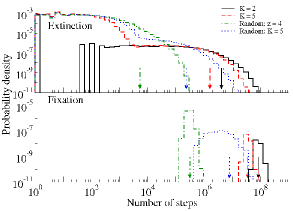
The various network topologies used in Fig. 1 recur throughout the paper, so we pause momentarily to introduce them. They are the $K$-funnel Lieberman et al. (2005), a random generalization thereof Barbosa et al. (2009), and the directed variant of the Erdős-Rényi random graphs Erdős and Rényi (1959) discussed in Karp (1990); Barbosa et al. (2003). For $b,K>1$ integers, the $K$-funnel of base $b$ has node set partitioned into $K$ subsets, called layers and numbered $0,1,\ldots,K-1$, such that there are $b^{k}$ nodes in layer $k$. The $K$-funnel, therefore, has $(b^{K}-1)/(b-1)$ nodes. For $k=1,2,\ldots,K-1$, an edge exists directed from each node in layer $k$ to each node in layer $k-1$. Additionally, an edge exists directed from the single node in layer $0$ to each of the nodes in layer $K-1$. The $K$-funnel is generalized by any network in which nodes occupy layers and edges exist only from all nodes in a layer to all nodes in the next according to some cyclic arrangement of the layers. The generalization we use Barbosa et al. (2009) is constructed randomly by first placing one node at each layer and then adding one extra node at a time to a layer that is chosen randomly with a bias that favors those layers that are nearest to the layer having the most nodes “upstream” from them. The other random networks we use Karp (1990); Barbosa et al. (2003) are such that a randomly chosen node has a number of out-neighbors given by the Poisson distribution of mean $z>1$ [so a giant strongly connected component (GSCC) is expected to exist with high probability]. The simulation of the evolutionary dynamics on such a network is confined to its GSCC.

We also remark, before proceeding, that some of our own recent work related to the fixation probability has been strongly influenced by the computational difficulties associated with estimating it. For example, in Barbosa et al. (2009) we set out to create a randomized growing mechanism for layered networks that would result in fitness amplifiers in the sense of Lieberman et al. (2005). The mechanism we created gives rise to the $K$-layer random networks introduced above and, indeed, we were able to demonstrate the desired amplification effect for $1\,000$ nodes. However, we fell short of demonstrating to full completion that the same holds for significantly larger networks, due mainly to the very large times required to compute the fixation probabilities of the thousands of candidate networks.

Our central concern in this paper is the devising of simulation strategies that can make the calculation of the fixation probability substantially faster while maintaining accuracy or reducing it only imperceptibly. We proceed along two tracks. The first is targeted at eliminating the evolutionary steps at which no change is effected to the number of mutants in the network. This occurs whenever the simulation prescribes that a mutant’s offspring is to replace another mutant or that a non-mutant’s offspring is to replace another non-mutant. Our results in this track are better suited to the layered networks introduced above; we demonstrate them for the $K$-funnel. The second track we pursue builds on the realization that, if in general it takes a lot more steps for fixation to occur than for extinction, then detecting early in the course of a simulation event that fixation is highly likely to occur can be used as a surrogate to the eventual detection of fixation and thereby reduce the number of necessary steps. We have found that, nearly regardless of the network for a large number of nodes, there exists a threshold number of mutants beyond which fixation is practically guaranteed to take place. We give results for a wide variety of networks.

We organize the remainder of the paper in the following manner. In Section II we briefly review the key notions related to the fixation probability. Then in Sections III and IV we pursue the two tracks outlined above for computing the fixation probability more efficiently, respectively for layered networks and for unrestricted networks. We conclude in Section V.

II Fixation probability

Let $P$ be a population of $n$ individuals and, for $i\in P$, let $P_{i}\subseteq P\setminus\{i\}$ be the set of individuals that an offspring of $i$ can replace during the evolution of $P$. Let also $Q_{i}$ be the set of individuals whose offspring can replace $i$. These give rise to a directed graph, called $D$, whose set of nodes is $P$ and whose set of edges, denoted by $E$, contains the edge $(i,j)$ if and only if $j\in P_{i}$ (equivalently, $i\in Q_{j}$). Each individual $i$ has a fitness $f_{i}>0$ associated with it, and similarly to each edge $(i,j)$ there corresponds a probability $w_{ij}$ such that $\sum_{j\in P_{i}}w_{ij}=1$ for all $i\in P$. The dynamics of evolution that we consider occurs in a sequence of steps. At each step, an individual $i$ is chosen with probability proportional to $f_{i}$, then another individual $j\in P_{i}$ is chosen with probability $w_{ij}$, and finally $j$ is replaced by an offspring of $i$ having fitness $f_{i}$.

The fixation probability of $D$, denoted by $\rho$, is the probability that a mutation spreads through all of $P$ given that it arises at one single individual and that all individuals in the remainder of the population have the same fitness. The value of $\rho$ depends on the structure of $D$ and on the ratio $r$ of the mutant’s fitness to that of the other individuals. Moreover, it is the relationship between $\rho$ and $r$ that determines whether evolution is driven primarily by natural selection or by random drift: essentially, natural selection predominates when $\rho$ and $r$ are highly correlated, random drift otherwise. Note in this context that, if $D$ is not strongly connected (i.e., there exist nodes $i$ and $j$ such that no directed path leads from $i$ to $j$), then $\rho>0$ if and only if there exists an individual from which all others are reachable. This may cause random drift to be the main driver of evolution, so henceforth we assume that $D$ is strongly connected (thus $\rho>0$ necessarily).

This type of evolutionary dynamics can be described by a discrete-time Markov chain of states $0,1,\ldots,n$, each representing a possible number of mutants in $D$. In this chain, states $0$ and $n$ are absorbing and all others are transient. If $s$ is a transient state, then from $s$ it is possible to move to state $s+1$ (with probability $p_{s}$), to state $s-1$ (with probability $q_{s}$), or to remain at state $s$ (with probability $1-p_{s}-q_{s}$). If we denote by $P_{n+1}(n\mid s)$ the probability that, having started at state $s$, this $(n+1)$-state system eventually enters state $n$, then it is well-known that

$$P_{n+1}(n\mid s)=\frac{1+\sum_{u=1}^{s-1}\prod_{v=1}^{u}q_{v}/p_{v}}{1+\sum_{u=1}^{n-1}\prod_{v=1}^{u}q_{v}/p_{v}}$$ (1)

(cf. El-Shehawey (2000) and references therein), whence $\rho$, which is given by $P_{n+1}(n\mid 1)$, is such that

$$\rho=\frac{1}{1+\sum_{u=1}^{n-1}\prod_{v=1}^{u}q_{v}/p_{v}}.$$ (2)

When the probabilities $w_{ij}$ are such that $\sum_{j\in Q_{i}}w_{ji}=1$ for all $i\in P$ (i.e., not only do the probabilities associated with the outgoing edges of $i$ sum up to $1$, but also those of the incoming edges), and only then, the isothermal theorem of Lieberman et al. (2005); Nowak (2006) establishes that $p_{v}/q_{v}=r$ for all $v\in\{1,2,\ldots,n-1\}$. In this case, and assuming that $r\neq 1$ (i.e., the mutation is either advantageous or disadvantageous, but not neutral), it follows from Eq. (2) that the fixation probability, now denoted by $\rho_{1}$, is

$$\rho_{1}=\frac{1-1/r}{1-1/r^{n}}.$$ (3)

This includes the Moran process Moran (1958), in which $D$ is such that $P_{i}=P\setminus\{i\}$ for all $i\in P$ and $w_{ij}=1/|P_{i}|$ for all $(i,j)\in E$ (we use $|X|$ to denote the cardinality of set $X$). It also includes the more general case in which the $w_{ij}$’s are thus constrained and, moreover, all nodes have as many incoming edges as outgoing edges, provided this number is the same for all nodes. Other noteworthy cases that also employ these locally uniform $w_{ij}$’s are the directed graphs that in Lieberman et al. (2005) are shown to be fitness amplifiers with respect to the expression for $\rho_{1}$. One example is the $K$-funnel, for which substituting $r^{K}$ for $r$ in Eq. (3) yields $\rho=\rho_{K}$ as $n\to\infty$, where

$$\rho_{K}=\frac{1-1/r^{K}}{1-1/r^{Kn}}.$$ (4)

III Fixation in layered networks

We henceforth use $w_{ij}=1/|P_{i}|$ for all $(i,j)\in E$ exclusively. For $t\geq 0$ an integer, let $E(t)\subset E$ be the set of edges $(i,j)$ such that, at the $t$th evolutionary step, node $i$ is a mutant but node $j$ is not. If $P^{+}(t)$ denotes the probability that, at step $t+1$, the number of mutants in $D$ increases (necessarily by $1$), then

$$P^{+}(t)=\sum_{(i,j)\in E(t)}\frac{r/|P_{i}|}{n+M(t)(r-1)},$$ (5)

where $M(t)$ is the number of mutants at step $t$ [so $M(0)=1$]. Letting $m_{i}(t)$ be an indicator of whether node $i$ is a mutant at step $t$ [i.e., $m_{i}(t)=1$ in the affirmative case, $0$ otherwise], this expression can be rewritten as a sum over all edges in $E$:

$$P^{+}(t) = \frac{r}{n+M(t)(r-1)}\sum_{(i,j)\in E}\frac{m_{i}(t)[1-m_{j}(t)]}{|P_{i}|}$$ (6)

$$= \frac{r}{n+M(t)(r-1)}$$ (8)

$$\left[\sum_{(i,j)\in E}\frac{m_{i}(t)}{|P_{i}|}-\sum_{(i,j)\in E}\frac{m_{i}(t)m_{j}(t)}{|P_{i}|}\right].$$

And since $D$ is strongly connected by assumption, we obtain

$$P^{+}(t)=\frac{r}{n+M(t)(r-1)}\left[M(t)-\sum_{(i,j)\in E}\frac{m_{i}(t)m_{j}(t)}{|P_{i}|}\right].$$ (9)

Similarly, the probability $P^{-}(t)$ that the number of mutants decreases (necessarily by $1$) at step $t+1$ is

$$P^{-}(t) = \frac{1}{n+M(t)(r-1)}$$ (11)

$$\left[\sum_{(i,j)\in E}\frac{m_{j}(t)}{|P_{i}|}-\sum_{(i,j)\in E}\frac{m_{i}(t)m_{j}(t)}{|P_{i}|}\right].$$

The number of mutants remains unchanged at step $t+1$ with probability $1-P^{+}(t)-P^{-}(t)$.

These expressions for $P^{+}(t)$ and $P^{-}(t)$ allow the evolutionary dynamics to be observed from some interesting perspectives. For example, any $D$ for which $\rho=\rho_{1}$ is such that $\sum_{(i,j)\in E}m_{j}(t)/|P_{i}|=\sum_{j\in P}m_{j}(t)\sum_{i\in Q_{j}}1/|P_{i}|=\sum_{j\in P}m_{j}(t)=M(t)$, and therefore $P^{+}(t)/P^{-}(t)=r=p_{s}/q_{s}$ for any state $s\in\{1,2,\ldots,n-1\}$ such that $M(t)=s$. This, essentially, is the argument behind the isothermal theorem. Moreover, for $r$ sufficiently close to $1$, what makes $P^{+}(t)$ and $P^{-}(t)$ differ from each other is the balance between $M(t)$ and $\sum_{(i,j)\in E}m_{j}(t)/|P_{i}|$, where the former does not depend on the topology of $D$ (given $t$) while the latter does. Thus, for example, if we consider the $K$-funnel and let $M_{k}(t)$ be the number of mutants in layer $k$ at step $t$, we have

$$\sum_{(i,j)\in E}\frac{m_{j}(t)}{|P_{i}|} = \sum_{k=0}^{K-2}\frac{M_{k}(t)b^{k+1}}{b^{k}}+\frac{M_{K-1}(t)}{b^{K-1}}$$ (12)

$$= b[M(t)-M_{K-1}(t)]+\frac{M_{K-1}(t)}{b^{K-1}}.$$ (13)

Readily, maintaining a relatively high value for the ratio $P^{+}(t)/P^{-}(t)$ (a strong forward bias) in the case of the $K$-funnel depends crucially on how close $M(t)$ and $M_{K-1}(t)$ are to each other, i.e., on how close the largest layer is to containing a significant fraction of the $M(t)$ mutants. The fact that $P^{+}(t)/P^{-}(t)\to r^{K}$ as $n\to\infty$ indicates that the topology of the $K$-funnel is in fact successful at maintaining the necessary distribution of mutants.

Equations (9) and (11) are also useful in that they provide an alternative mechanism for simulating the evolutionary dynamics. Instead of repeatedly choosing $i$, then $j\in P_{i}$ to receive $i$’s offspring, until the mutation either spreads through the whole of $D$ or dies out, we use the two equations to decide, at each step $t$, whether the number of mutants will increase, decrease, or remain the same at step $t+1$. In the former two cases we choose the nodes to be involved, create or destroy a mutant as the case may be, then compute $P^{+}(t+1)$ and $P^{-}(t+1)$. By doing so, all steps in which no mutant is created or destroyed are skipped. Of course, in order for this alternative to be computationally attractive the suppression of these steps has to compensate for the additional effort to calculate the probabilities at every step that is not suppressed.

While it is unclear that this will be so in the general case, for layered networks like the $K$-funnel, in which all nodes in the same layer are topologically identical to one another (they all have the same in- and out-neighbors), the simulation can be conducted by keeping track only of the number of mutants in each layer and the alternative becomes attractive. We then consider the generalization of the $K$-funnel obtained by letting layer $k$ have any number $n_{k}>0$ of nodes. In this case, we can rewrite Eqs. (9) and (11) by decomposing each of $P^{+}(t)$ and $P^{-}(t)$ into $K$ summands, each related to a pair of subsequent layers. Thus, we obtain $P^{+}(t)=\sum_{k=0}^{K-1}P_{k}^{+}(t)$ and $P^{-}(t)=\sum_{k=0}^{K-1}P_{k}^{-}(t)$, with

$$P_{k}^{+}(t)=\frac{rM_{k+1}(t)[n_{k}-M_{k}(t)]}{n_{k}[n+M(t)(r-1)]}$$ (14)

and

$$P_{k}^{-}(t)=\frac{M_{k}(t)[n_{k+1}-M_{k+1}(t)]}{n_{k}[n+M(t)(r-1)]},$$ (15)

where $M_{k}(t)$ is as for the $K$-funnel. In these expressions, and henceforth, layer numbers are incremented or decremented modulo $K$.

For layered networks such as these, once it has been decided that a mutant is to be created or destroyed at step $t+1$, the layer at which this is to happen is $k$ with probability proportional to $P_{k}^{+}(t)$, in the case of creation, or $P_{k}^{-}(t)$, in the case of destruction [consistently with this, notice that $P_{k}^{+}(t)=0$ if $M_{k+1}(t)=0$ or $M_{k}(t)=n_{k}$, and that $P_{k}^{-}(t)=0$ if $M_{k}(t)=0$ or $M_{k+1}(t)=n_{k+1}$]. And once $M_{k}(t+1)$ has been updated from $M_{k}(t)$, it follows from Eqs. (14) and (15) that only $P_{k}^{+}(t+1)$ and $P_{k-1}^{+}(t+1)$, or $P_{k}^{-}(t+1)$ and $P_{k-1}^{-}(t+1)$, need to be calculated. This is so because, although $M(t+1)$ is updated from $M(t)$ as well, the only effect this has is to alter the factor in the denominator of Eqs. (14) and (15) that is common to all layers. As a consequence, the probabilities corresponding to any layer other than $k$ or $k-1$ need not be calculated.

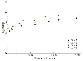
Computational results on the $K$-funnel are given in Fig. 2 for a variety of $n$ and $K$ values, where we show the speedup afforded by the use of Eqs. (14) and (15) to compute the fixation probability. This speedup is defined in terms of processor time and indicates, in all cases examined, a reduction to less than half the time required by the simulation that goes through all the evolutionary steps. We note, however, that the approach we discuss in Section IV allows for much more significant speedups.

Figure 2: (Color online) Speedups resulting from the use of Eqs. (14) and (15) on the $K$-funnel with $r=1.1$. Data are averages over at least $10^{4}$ events.

IV Fixation in arbitrary networks

In the absence of the computational facilitation provided by layered networks, which as we have seen allows the fixation probability to be computed more efficiently by skipping all steps of the simulation in which no mutant is created or destroyed, for an unrestricted topology we turn to the alternative strategy of attempting an early stop of each simulation event based on how many mutants there are. The central question is whether there exists a threshold number of mutants which, once crossed from below, ensures that fixation is bound to occur with probability as close to $1$ as one wishes. We provide an affirmative answer in what follows.

The probability that the mutation eventually dies out, given that $s$ mutants are originally present, equals $1-P_{n+1}(n\mid s)$. We denote it by $Q_{n+1}(0\mid s)$, and it follows from Eq. (1) that

$$Q_{n+1}(0\mid s)=\frac{\sum_{u=s}^{n-1}\prod_{v=1}^{u}q_{v}/p_{v}}{1+\sum_{u=1}^{n-1}\prod_{v=1}^{u}q_{v}/p_{v}}.$$ (16)

We are interested in the probability that, conditioned on the fact that extinction does actually occur, the number of mutants eventually grows from the initial $s$ to some fixed value $M\in\{s,s+1,\ldots,n-1\}$ but does not surpass it. We denote this probability by $Q_{n+1}^{M}(0\mid s)$ and remark that, should its dependency with $M$ be known, we would immediately be able to discover the desired threshold for the number of mutants by adopting $s=1$ and specifying a lower bound on the probability. In other words, we would discover the threshold, call it $M^{*}$, by specifying $Q^{*}$ such that $Q_{n+1}^{M}(0\mid 1)\geq Q^{*}$ for all $M\leq M^{*}$. This follows from the intuitive expectation that $Q_{n+1}^{M}(0\mid s)$ is to decrease as $M$ grows for sufficiently large $M$.

From its definition as a conditional probability, $Q_{n+1}^{M}(0\mid s)$ is given by $AB/Q_{n+1}(0\mid s)$, where $A$ is the probability that the number of mutants in the network eventually increases from $s$ to $M$ and $B$ is the probability that, given that it has $M$ mutants, the system eventually returns to state $0$ without ever increasing its number of mutants beyond $M$. We calculate the values of $A$ and $B$ by resorting to discrete-time Markov chains entirely analogous to the one we have been using, but now having reduced numbers of states. The first of these chains has states $0,1,\ldots,M$, of which $0$ and $M$ are absorbing while all else remains unchanged. We set $A$ to the probability that the system gets absorbed into state $M$ having started at state $s$, that is, $A=P_{M+1}(M\mid s)$. The second chain has states $0,1,\ldots,M+1$, with $0$ and $M+1$ the absorbing states and everything else unchanged. We set $B$ to the probability that absorption occurs at state $0$ once the system is started at state $M$, that is, $B=Q_{M+2}(0\mid M)$. We then obtain

$$Q_{n+1}^{M}(0\mid s)=\frac{P_{M+1}(M\mid s)Q_{M+2}(0\mid M)}{Q_{n+1}(0\mid s)}.$$ (17)

Closed-form expressions are in general not known for Eqs. (1) or (16), so we assume that it suffices to consider the case in which $p_{v}/q_{v}=r$ for all transient states $v$. In this case, and for $r\neq 1$, Eq. (17) yields

$$Q_{n+1}^{M}(0\mid s)=\frac{(1-1/r^{s})(1-1/r)}{(1-1/r^{M})(1-1/r^{M+1})r^{M}}\frac{1-1/r^{n}}{1/r-1/r^{n}}.$$ (18)

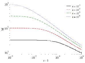
Readily, $Q_{n+1}^{M}(0\mid s)$ becomes independent of $n$ as $n$ grows, regardless of whether $r>1$ or $r<1$ (but note that the two limits differ). For $n\to\infty$, in Fig. 3 we show plots of $Q_{n+1}^{M}(0\mid 1)=\epsilon$ for different values of $\epsilon$ and $1<r\leq 2$. As expected, for fixed $\epsilon$ the value of $M$ increases with decreasing $r$ in this range, and somewhat counterintuitively we see that the rate of increase is ever smaller as $r$ approaches $1$. However, this is easily confirmed as we realize that, as in the figure, the limit $Q$ of $Q_{n+1}^{M}(0\mid 1)$ as $r\to 1$ is such that $M\approx\sqrt{1/Q}$.

Figure 3: (Color online) $M$ as a function of $r$ for $Q_{n+1}^{M}(0\mid 1)=\epsilon$.

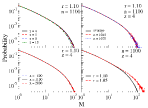
Computational results on the distribution of $M$, the maximum number of mutants achieved when the dynamics ends in extinction, are given in Figs. 4 through 6 for a variety of topologies. Figure 4 refers to the $K$-funnel, Fig. 5 to random networks with a Poisson-distributed number of out-neighbors, and Fig. 6 to a selection of networks that includes an instance of each of these two types and also the unidirectional ring. The latter figure also includes plots of the analytical prediction given by Eq. (18). In this respect, notice that the prediction that corresponds to the $r$ value used in the simulations matches the data for the unidirectional ring perfectly. This, of course, is consistent with the fact that, in this case, the requirements of the isothermal theorem are satisfied and therefore the assumption behind Eq. (18) is exact. Similarly, in the figure’s inset we demonstrate that, for the random network in use, the prediction of Eq. (18) with a slightly lower value of $r$ is also a perfect match.

Figure 4: (Color online) Probability distributions of $M$ for the $K$-funnel. Data are averages over $10^{6}$ events.

Figure 5: (Color online) Probability distributions of $M$ for random networks with a Poisson-distributed number of out-neighbors. Data are averages over $10^{7}$ events ($10^{4}$ events for each of $10^{3}$ graphs with at least $0.95n$ nodes in the GSCC). The plot labeled “average” refers to all data for $r=1.1$, $n=1\,100$, and $z=4$ in all panels. This is compared in the same panel to the results corresponding to a single graph whose GSCC has $1\,045$ or $1\,070$ nodes, for which $10^{6}$ events have been run.

Figure 6: (Color online) Probability distributions of $M$ for assorted topologies with $r=1.1$. Data are averages over $10^{6}$ events for the $K$-funnel and the unidirectional ring, $10^{7}$ events for the random network ($10^{4}$ events for each of $10^{3}$ graphs with at least $0.95n$ nodes in the GSCC).

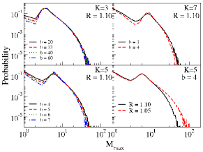
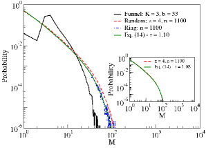
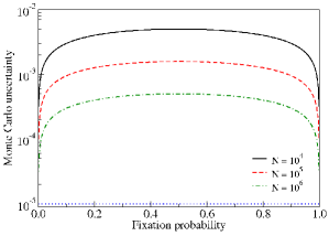
Notice also, in all three figures, that for $M=100$ no probability is above $10^{-5}$. This means that, during the simulations, of all events that ended in extinction, no more than one out of $10^{5}$ achieved more than $100$ mutants. As a consequence, should we use $M^{*}=100$ (corresponding roughly to $Q^{*}=10^{-6}$, given that there were at least $10^{6}$ events) and count as an event ending in fixation any event achieving more than $M^{*}$ mutants, we would be introducing a deviation of no more than $10^{-5}$ with respect to the actual value of the fixation probability. But the fixation probability obtained by full simulations of the evolutionary dynamics is itself subject to the so-called standard error that is inherent to any Monte Carlo simulation. If $\hat{\rho}$ denotes the fixation probability calculated after $N$ events, then the standard error is the standard deviation of the $0$’s (extinctions) and $1$’s (fixations) accumulated along the events divided by $\sqrt{N}$, that is, $\sqrt{\hat{\rho}(1-\hat{\rho})/N}$. This function of $\hat{\rho}$ is plotted in Fig. 7 for different values of $N$, along with a flat line for the constant $10^{-5}$. Clearly, the additional deviation introduced by the use of $M^{*}=100$ is negligible when compared to the standard error.

Figure 7: (Color online) Inherent uncertainty associated with the Monte Carlo computations of the fixation probability, as given by the standard error of the fixation probability estimate $\hat{\rho}$.

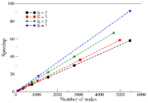
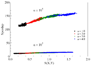
Speedup figures resulting from the use of early fixation detection for $M^{*}=100$ are shown in Figs. 8 and 9, respectively for the $K$-funnel (with several $n$ and $K$ values) and the $K$-layer random networks of Barbosa et al. (2009) (with two values of $n$, $K=5$, and several values of the $a$ parameter that in Barbosa et al. (2009) is used to control the layer-selection mechanism as the network is grown by the addition of new nodes). Plots in the latter figure are given against $S(X,Y)$, which in Barbosa et al. (2009) is used to indicate, if sufficiently above $0$, how close each network is to having, like the $K$-funnel, an exponentially growing number of nodes per layer as one moves “upstream” through the layers. Clearly, speedups are very significant, particularly for the $K$-funnel with the largest values of $n$ and $K$ and all random networks of $10\,000$ nodes. We also remark that, in Fig. 8, the fact that slopes increase with $K$ is closely related to Eq. (4): as the fraction of events that lead to fixation grows with $K$, we expect from Fig. 1 that the average number of steps behave likewise; qualitatively, this explains why speedups increase with $K$.

Figure 8: (Color online) Speedups resulting from the use of the $M^{*}=100$ threshold on the $K$-funnel with $r=1.1$. Data are averages over $10^{6}$ events.

Figure 9: (Color online) Speedups resulting from the use of the $M^{*}=100$ threshold on the random networks of Barbosa et al. (2009) with $r=1.1$. Data are averages over $10^{7}$ events ($10^{4}$ events for each of $10^{3}$ graphs), except for $n=10\,000$ with $a=4$, in which case $10^{4}$ events are used for each of $500$ graphs.

V Final remarks

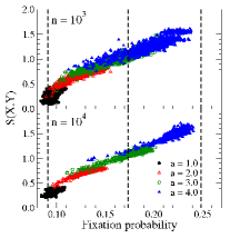
In Section I we mentioned that, in Barbosa et al. (2009), we were unable to extend to larger values of $n$ our conclusions regarding the fitness-amplification properties of the $K$-layer random networks we used in some of this paper’s experiments. Provisioned with the technique of Section IV, we can now bypass the computational difficulties that hampered our progress in that occasion by employing early detection of fixation. Doing this for $M^{*}=100$ has resulted in the data shown in Fig. 10, from which it is finally clear that, also for $n=10\,000$, it is possible to grow layered networks that achieve significant fitness amplification. As we see in the figure, for $K=5$ many grown networks have $\rho$ values between $\rho_{2}$ and $\rho_{3}$. We note, however, that this is still an easier scenario than that of Barbosa et al. (2009), where $K=10$ was used for $n=10\,000$, since in the present case we had to calculate the speedups given in Fig. 9 and these required that simulation events be carried out to completion.

Figure 10: (Color online) Results for the random networks of Barbosa et al. (2009) with $K=5$ and $r=1.1$. Each graph whose layer populations correlate with those of the $K$-funnel by more than $0.9$ in the sense of the Pearson correlation coefficient is represented by its fixation probability and its $S(X,Y)$ value. Data are averages over $10^{7}$ events ($10^{4}$ events for each of $10^{3}$ graphs), except for $n=10\,000$ with $a=4$, in which case $10^{4}$ events are used for each of $500$ graphs. Dashed lines indicate $\rho=\rho_{1}$ through $\rho_{3}$.

Another interesting by-product of our use of the threshold number of mutants $M^{*}$ is that, should the dynamics be started with $s>M^{*}$ randomly placed mutants of equal fitness, then fixation would occur almost surely. This is so because the probability of there being so many mutants in a dynamics that is bound to extinction is as small as allowed by the choice of $Q^{*}$. However, note that Eq. (18) is of no immediate help in quantifying the “almost surely,” since it is conditioned on the dynamics ending in extinction and therefore does not apply to those cases in which the number of mutants becomes large enough that extinction is unlikely. Nevertheless, whenever the isothermal theorem holds, Eq. (1) implies that fixation from the initial $s$ mutants occurs with probability $(1-1/r^{s})/(1-1/r^{n})$ (see also Lieberman et al. (2005)), which is asymptotically equal to $1$ for $r>1$ as both $s$ and $n$ grow.

It is also worth mentioning that, because this study has been targeted at directed graphs, Eqs. (9) and (11) are also applicable to the special case of an undirected graph and can lead to useful insight also in this case. Specifically, suppose we take any strongly connected $D$ without antiparallel edges and make it functionally undirected by adding to it the antiparallel counterpart of every one of its edges. If $E$ and the $P_{i}$ sets continue to refer to the original $D$, then the contribution of each mutant $l$ to $\sum_{(i,j)\in E}m_{j}(t)/|P_{i}|$ in Eq. (11) jumps from $\sum_{(i,l)\in E}1/|P_{i}|$ to $\sum_{(i,l)\in E}1/|P_{i}|+\sum_{(l,i)\in E}1/|P_{i}|$, therefore leading to a smaller $P^{+}(t)/P^{-}(t)$ ratio. On the other hand, if $D$ already has antiparallel edges, then one curious special case is that of the $2$-superstar of Lieberman et al. (2005), which has a central node with $n-1$ peripheral nodes that connect to it through antiparallel edge pairs. This graph is already functionally undirected and, for $n\to\infty$, $\rho\to\rho_{2}$. So the $2$-superstar is somewhat of an exception with regard to the $P^{+}(t)/P^{-}(t)$ ratio for undirected graphs. In fact, thus far we have been unable to find any other undirected graphs for which $\rho\geq\rho_{2}$, but to the best of our knowledge the question of whether any exist remains unsettled.

We note, finally, that fixation for the $2$-superstar, when it happens, is bound to take a considerable number of steps to occur (this can be seen in Fig. 1, since the $2$-superstar and the $2$-funnel with the same number of nodes are the same graph). For the $2$-superstar, the sum from Eq. (11) mentioned above is $M_{\mathrm{p}}(t)/(n-1)+m_{\mathrm{c}}(t)(n-1)$, where $M_{\mathrm{p}}(t)$ is the number of peripheral mutants at step $t$ and $m_{\mathrm{c}}(t)$ is either $1$ or $0$, indicating respectively whether or not a central mutant exists at that step. Clearly, for $r$ only slightly above $1$, obtaining $P^{+}(t)>P^{-}(t)$ depends crucially on the existence of the central mutant. This, in turn, can easily change from step to step until fixation is eventually approached. It is precisely in cases such as this that the early estimates of the fixation probability introduced in Section IV are most useful.