Testing Bell inequalities with weak measurements

Shmuel Marcovitch and Benni Reznik School of Physics and Astronomy, Raymond and Beverly Sackler Faculty of Exact Sciences, Tel-Aviv University, Tel-Aviv 69978, Israel.
Abstract

Quantum theory is inconsistent with any local hidden variable model as was first shown by Bell. To test Bell inequalities two separated observers extract correlations from a common ensemble of identical systems. Since quantum theory does not allow simultaneous measurements of noncommuting observables, on each system every party measures a single randomly chosen observable out of a given set. Here we suggest a different approach for testing Bell inequalities that is experimentally realizable by current methods. We show that Bell inequalities can be maximally violated even when all observables are measured on each member of the ensemble. This is possible by using weak measurements that produce small disturbance, at the expense of accuracy. However, our approach does not constitute an independent test of quantum nonlocality since the local hidden variables may correlate the noise of the measurement instruments. Nevertheless, by adding a randomly chosen precise measurement at the end of every cycle of weak measurements, the parties can verify that the hidden variables were not interfering with the noise, and thus validate the suggested test.

I Introduction

Quantum nonlocality bell has been tested aspect ; zeilinger in different systems and is now widely accepted. Its most simple manifestation is given by Clauser-Horne-Shimony-Holt (CHSH) inequality chsh , in which every cycle A𝐴A and B𝐡B measure one out of two randomly chosen observables a1,a2∈{Β±1}subscriptπ‘Ž1subscriptπ‘Ž2plus-or-minus1a_{1},a_{2}\in\{\pm 1\} and b1,b2∈{Β±1}subscript𝑏1subscript𝑏2plus-or-minus1b_{1},b_{2}\in\{\pm 1\}. In a local hidden variable model B≀2𝐡2B\leq 2, where

B=|E​(a1​b1)+E​(a1​b2)+E​(a2​b1)βˆ’E​(a2​b2)|.𝐡𝐸subscriptπ‘Ž1subscript𝑏1𝐸subscriptπ‘Ž1subscript𝑏2𝐸subscriptπ‘Ž2subscript𝑏1𝐸subscriptπ‘Ž2subscript𝑏2B=|E(a_{1}b_{1})+E(a_{1}b_{2})+E(a_{2}b_{1})-E(a_{2}b_{2})|. (1)

Above E​(ai​bj)𝐸subscriptπ‘Žπ‘–subscript𝑏𝑗E(a_{i}b_{j}) is the joint expectation value. The EPR state

|ψ⟩=12(|↑zA↑zB⟩+|↓zA↓zB⟩),|\psi\rangle=\frac{1}{\sqrt{2}}(|\uparrow^{A}_{z}\uparrow^{B}_{z}\rangle+|\downarrow^{A}_{z}\downarrow^{B}_{z}\rangle), (2)

saturates the maximal bound 2​2222\sqrt{2} tsirelson with i.e. a1=Οƒxsubscriptπ‘Ž1subscript𝜎π‘₯a_{1}=\sigma_{x}, a2=Οƒzsubscriptπ‘Ž2subscriptπœŽπ‘§a_{2}=\sigma_{z}, b1=σπ/4subscript𝑏1subscriptπœŽπœ‹4b_{1}=\sigma_{\pi/4}, and b2=Οƒ3​π/4subscript𝑏2subscript𝜎3πœ‹4b_{2}=\sigma_{3\pi/4}, where σπ/4=12​(Οƒx+Οƒz)subscriptπœŽπœ‹412subscript𝜎π‘₯subscriptπœŽπ‘§\sigma_{\pi/4}=\frac{1}{\sqrt{2}}(\sigma_{x}+\sigma_{z}) and Οƒ3​π/4=12​(Οƒxβˆ’Οƒz)subscript𝜎3πœ‹412subscript𝜎π‘₯subscriptπœŽπ‘§\sigma_{3\pi/4}=\frac{1}{\sqrt{2}}(\sigma_{x}-\sigma_{z}).

Refer to caption
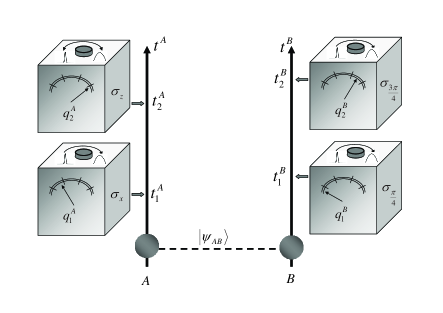
Figure 1: Sequential CHSH setup. Parties A𝐴A and B𝐡B measure two observables at sequential times. The knobs control the inaccuracy of the devices. In the accurate measurement limit the pointer readings correspond to the possible values of the observables (Β±1plus-or-minus1\pm 1). In the inaccurate (weak) limit the readings are noisy, and the microscopic values cannot be inferred. We require that the distance between the parties d=|XAβˆ’XB|𝑑subscript𝑋𝐴subscript𝑋𝐡d=|X_{A}-X_{B}| satisfies dβ‰ͺc​t2Amuch-less-than𝑑𝑐superscriptsubscript𝑑2𝐴d\ll ct_{2}^{A} and dβ‰ͺc​t2Bmuch-less-than𝑑𝑐superscriptsubscript𝑑2𝐡d\ll ct_{2}^{B}.

In the regular setting every cycle the parties measure a single observable. In our approach to be referred to as the sequential setting, for each member of the ensemble A𝐴A measures both a1subscriptπ‘Ž1a_{1} and a2subscriptπ‘Ž2a_{2} (one after another), and similarly B𝐡B measures both b1subscript𝑏1b_{1} and b2subscript𝑏2b_{2}, as is schematically described in Fig. 1. Obviously, as discussed above, for ordinary measurements the first measurement of a1subscriptπ‘Ž1a_{1} would randomize the result in the subsequent measurement of a2subscriptπ‘Ž2a_{2}, and no violation of Bell inequalities would be manifested. However, as is well known, there is a trade-off between the accuracy of the measurement and the disturbance caused to the system von . The limit in which individual measurements provide vanishing information gain was first analyzed by Aharonov et. al. (in the context of post-selection) weak and was termed weak measurements. In this limit the measurements become inaccurate and one could expect that nonlocal correlations would not be observed.

The main result of this paper is that as one gradually reduces the disturbance caused to the system, by decreasing the accuracy of measurements, one in fact regains the maximal violation of Bell inequalities. This result is stated in theorem 1 and corollary 1. The outcomes of inaccurate measurements may lie outside the usual range of the measured observables. In this case local hidden variables may interfere with the noise to violate Bell inequalities. Therefore our approach does not constitute an independent test of quantum nonlocality. However, by adding a single randomly chosen precise measurement at the end of each cycle, the parties can determine whether the hidden variables interfere with the noise. The expected negative result implies that the inaccurate measurements still provide a valid test. This is manifested in corollary 2. We then proceed by quantitatively illustrating the transition from strong to weak measurements in the sequential setting in realistic finite ensembles and show that simultaneously different Bell tests can be attained using the same ensemble. We conclude by discussing implications of our approach, in particular maximal violation of the Leggett and Garg inequalities leggett and possible realizations of the suggested method.

II Violation of Bell inequalities with weak measurements

Theorem 1. Let a system |ψ⟩ketπœ“|\psi\rangle be measured sequentially by an arbitrary number of observables Oisubscript𝑂𝑖O_{i} (i=1,…,m𝑖1β€¦π‘ši=1,\dots,m) at times tisubscript𝑑𝑖t_{i} where 0<t1<t2<β‹―<tm0subscript𝑑1subscript𝑑2β‹―subscriptπ‘‘π‘š0<t_{1}<t_{2}<\cdots<t_{m}. In the limit of weak measurements,

EQ​M​(qi)=⟨ψ|Oi​(ti)|ψ⟩,subscript𝐸𝑄𝑀subscriptπ‘žπ‘–quantum-operator-productπœ“subscript𝑂𝑖subscriptπ‘‘π‘–πœ“\displaystyle E_{QM}(q_{i})=\langle\psi|O_{i}(t_{i})|\psi\rangle, (3)
EQ​M​(qi​qj)=Reβ€‹βŸ¨Οˆ|Oi​(ti)​Oj​(tj)|ψ⟩,subscript𝐸𝑄𝑀subscriptπ‘žπ‘–subscriptπ‘žπ‘—Requantum-operator-productπœ“subscript𝑂𝑖subscript𝑑𝑖subscript𝑂𝑗subscriptπ‘‘π‘—πœ“\displaystyle E_{QM}(q_{i}q_{j})=\mbox{Re}\langle\psi|O_{i}(t_{i})O_{j}(t_{j})|\psi\rangle, (4)

where qisubscriptπ‘žπ‘–q_{i} is the reading of the i𝑖ith measurement apparatus pointer. The observables Oisubscript𝑂𝑖O_{i} are written in the Heisenberg representation, Oi​(ti)≑U†​(ti)​Oi​U​(ti)subscript𝑂𝑖subscript𝑑𝑖superscriptπ‘ˆβ€ subscript𝑑𝑖subscriptπ‘‚π‘–π‘ˆsubscript𝑑𝑖O_{i}(t_{i})\equiv U^{\dagger}(t_{i})O_{i}U(t_{i}), U​(t)=eβˆ’i​H0​tπ‘ˆπ‘‘superscript𝑒𝑖subscript𝐻0𝑑U(t)=e^{-iH_{0}t}, and H0subscript𝐻0H_{0} is the free Hamiltonian.

Proof. The full Hamiltonian is

H=H0+βˆ‘imδ​(tβˆ’ti)​pi​Oi,𝐻subscript𝐻0superscriptsubscriptπ‘–π‘šπ›Ώπ‘‘subscript𝑑𝑖subscript𝑝𝑖subscript𝑂𝑖H=H_{0}+\sum_{i}^{m}\delta(t-t_{i})p_{i}O_{i}, (5)

where [qi,pi]=isubscriptπ‘žπ‘–subscript𝑝𝑖𝑖[q_{i},p_{i}]=i (we take ℏ=1Planck-constant-over-2-pi1\hbar=1). The second term in Eq. (5) corresponds to the von-Neumann measurement interaction, where for simplicity instantaneous measurements are assumed. In addition, we assume identical initial Gaussian wavepackets for the pointers:

ϕ​(qi,t=0)=(Ο΅2​π)1/4​eβˆ’Ο΅β€‹qi2/4,italic-Ο•subscriptπ‘žπ‘–π‘‘0superscriptitalic-Ο΅2πœ‹14superscript𝑒italic-Ο΅superscriptsubscriptπ‘žπ‘–24\phi(q_{i},t=0)=\left(\frac{\epsilon}{2\pi}\right)^{1/4}e^{-\epsilon q_{i}^{2}/4}, (6)

where Ο΅βˆ’1=[Δ​qi​(t=0)]2≑σ2superscriptitalic-Ο΅1superscriptdelimited-[]Ξ”subscriptπ‘žπ‘–π‘‘02superscript𝜎2\epsilon^{-1}=[\Delta q_{i}(t=0)]^{2}\equiv\sigma^{2}. The initial state of the system and the apparatuses

|Ψ⟩=|ΟˆβŸ©βŠ—βˆiϕ​(qi),ketΞ¨tensor-productketπœ“subscriptproduct𝑖italic-Ο•subscriptπ‘žπ‘–|\Psi\rangle=|\psi\rangle\otimes\prod_{i}\phi(q_{i}), (7)

evolves in time according to

𝒰=∏i𝒰iβ‰‘βˆiU†​(ti)​eβˆ’i​pi​Oi​U​(ti).𝒰subscriptproduct𝑖subscript𝒰𝑖subscriptproduct𝑖superscriptπ‘ˆβ€ subscript𝑑𝑖superscript𝑒𝑖subscript𝑝𝑖subscriptπ‘‚π‘–π‘ˆsubscript𝑑𝑖{\cal U}=\prod_{i}{\cal U}_{i}\equiv\prod_{i}U^{\dagger}(t_{i})e^{-ip_{i}O_{i}}U(t_{i}). (8)

Each operation of p𝑝p yields an order of Ο΅italic-Ο΅\epsilon. In the limit of weak measurements, the inaccuracy Οƒβ†’βˆžβ†’πœŽ\sigma\to\infty (Ο΅β†’0β†’italic-Ο΅0\epsilon\to 0).

By expanding 𝒰isubscript𝒰𝑖{\cal U}_{i} to first order in Ο΅italic-Ο΅\epsilon, while keeping terms to first order in 𝒰𝒰{\cal U} and tracing out the system and qjsubscriptπ‘žπ‘—q_{j}, jβ‰ i𝑗𝑖j\neq i, one obtains Eq. (3).

To derive Eq. (4) we expand to second order

eβˆ’i​pi​Oi=1βˆ’i​pi​Oiβˆ’12​pi2​Oi2+o​(Ο΅3).superscript𝑒𝑖subscript𝑝𝑖subscript𝑂𝑖1𝑖subscript𝑝𝑖subscript𝑂𝑖12superscriptsubscript𝑝𝑖2superscriptsubscript𝑂𝑖2π‘œsuperscriptitalic-Ο΅3e^{-ip_{i}O_{i}}=1-ip_{i}O_{i}-\frac{1}{2}p_{i}^{2}O_{i}^{2}+o(\epsilon^{3}).

After the measurements the state of the systems and the pointers is given by

|Ψ⟩=U(tm)[∏lmΟ•(ql)βˆ’βˆ‘kmΟ•β€²(qk)∏lβ‰ kΟ•(ql)Ok(tk)+βˆ‘k<lϕ′​(qk)​ϕ′​(ql)β€‹βˆsβ‰ k,lϕ​(qs)​Ol​(tl)​Ok​(tk)+12βˆ‘kmΟ•β€²β€²(qk)∏lβ‰ kΟ•(ql)Ok2(tk)+o(Ο΅3)]|ψ⟩.ketΞ¨π‘ˆsubscriptπ‘‘π‘šdelimited-[]superscriptsubscriptproductπ‘™π‘šitalic-Ο•subscriptπ‘žπ‘™superscriptsubscriptπ‘˜π‘šsuperscriptitalic-Ο•β€²subscriptπ‘žπ‘˜subscriptproductπ‘™π‘˜italic-Ο•subscriptπ‘žπ‘™subscriptπ‘‚π‘˜subscriptπ‘‘π‘˜subscriptπ‘˜π‘™superscriptitalic-Ο•β€²subscriptπ‘žπ‘˜superscriptitalic-Ο•β€²subscriptπ‘žπ‘™subscriptproductπ‘ π‘˜π‘™italic-Ο•subscriptπ‘žπ‘ subscript𝑂𝑙subscript𝑑𝑙subscriptπ‘‚π‘˜subscriptπ‘‘π‘˜12superscriptsubscriptπ‘˜π‘šsuperscriptitalic-Ο•β€²β€²subscriptπ‘žπ‘˜subscriptproductπ‘™π‘˜italic-Ο•subscriptπ‘žπ‘™superscriptsubscriptπ‘‚π‘˜2subscriptπ‘‘π‘˜π‘œsuperscriptitalic-Ο΅3ketπœ“\begin{split}|\Psi\rangle\!&=U(t_{m})\!\Big{[}\prod_{l}^{m}\!\phi(q_{l})\!-\sum_{k}^{m}\!\phi^{\prime}(q_{k})\prod_{l\neq k}\phi(q_{l})O_{k}(t_{k})\!\\ &+\sum_{k<l}\!\phi^{\prime}(q_{k})\phi^{\prime}(q_{l})\!\prod_{s\neq k,l}\!\phi(q_{s})O_{l}(t_{l})O_{k}(t_{k})\\ &+\frac{1}{2}\sum_{k}^{m}\!\phi^{\prime\prime}(q_{k})\prod_{l\neq k}\!\phi(q_{l})O_{k}^{2}(t_{k})\!+\!o(\epsilon^{3})\!\Big{]}\!|\psi\rangle.\end{split} (9)

Let us compute EQ​M​(qi​qj)subscript𝐸𝑄𝑀subscriptπ‘žπ‘–subscriptπ‘žπ‘—E_{QM}(q_{i}q_{j}), where without loss of generality i<j𝑖𝑗i<j. Define U​(tj)​|ΟˆβŸ©π‘ˆsubscript𝑑𝑗ketπœ“U(t_{j})|\psi\rangle =βˆ‘Ξ΄r​|ψr⟩absentsubscriptπ›Ώπ‘Ÿketsubscriptπœ“π‘Ÿ=\,\sum\delta_{r}|\psi_{r}\rangle, U​(tj)​Ok​(tk)​|ΟˆβŸ©π‘ˆsubscript𝑑𝑗subscriptπ‘‚π‘˜subscriptπ‘‘π‘˜ketπœ“U(t_{j})O_{k}(t_{k})|\psi\rangle =βˆ‘Ξ±rk​|ψr⟩absentsubscriptsuperscriptπ›Όπ‘˜π‘Ÿketsubscriptπœ“π‘Ÿ=\,\sum\alpha^{k}_{r}|\psi_{r}\rangle, and U​(tj)​Ol​(tl)​Ok​(tk)​|ΟˆβŸ©π‘ˆsubscript𝑑𝑗subscript𝑂𝑙subscript𝑑𝑙subscriptπ‘‚π‘˜subscriptπ‘‘π‘˜ketπœ“U(t_{j})O_{l}(t_{l})O_{k}(t_{k})|\psi\rangle =βˆ‘Ξ·rk​l​|ψr⟩absentsubscriptsuperscriptπœ‚π‘˜π‘™π‘Ÿketsubscriptπœ“π‘Ÿ=\,\sum\eta^{kl}_{r}|\psi_{r}\rangle, where |ψr⟩ketsubscriptπœ“π‘Ÿ|\psi_{r}\rangle is any basis and k,l≀jπ‘˜π‘™π‘—k,l\leq j. Expanding Eq. (9) in the |ψr⟩ketsubscriptπœ“π‘Ÿ|\psi_{r}\rangle basis up to the j𝑗jth measurement yields

|Ψ⟩=βˆ‘r[Ξ΄r∏kjΟ•(qk)βˆ’βˆ‘kjΞ±rkΟ•β€²(qk)∏lβ‰ kΟ•(ql)+βˆ‘k<lϕ′​(qk)​ϕ′​(ql)β€‹βˆsβ‰ k,lϕ​(qs)​ηrk​l+12βˆ‘kjΟ•β€²β€²(qk)∏lβ‰ kΟ•(ql)Ξ·rk​k+o(Ο΅3)]|ψr⟩.ketΞ¨subscriptπ‘Ÿdelimited-[]subscriptπ›Ώπ‘Ÿsuperscriptsubscriptproductπ‘˜π‘—italic-Ο•subscriptπ‘žπ‘˜superscriptsubscriptπ‘˜π‘—subscriptsuperscriptπ›Όπ‘˜π‘Ÿsuperscriptitalic-Ο•β€²subscriptπ‘žπ‘˜subscriptproductπ‘™π‘˜italic-Ο•subscriptπ‘žπ‘™subscriptπ‘˜π‘™superscriptitalic-Ο•β€²subscriptπ‘žπ‘˜superscriptitalic-Ο•β€²subscriptπ‘žπ‘™subscriptproductπ‘ π‘˜π‘™italic-Ο•subscriptπ‘žπ‘ subscriptsuperscriptπœ‚π‘˜π‘™π‘Ÿ12superscriptsubscriptπ‘˜π‘—superscriptitalic-Ο•β€²β€²subscriptπ‘žπ‘˜subscriptproductπ‘™π‘˜italic-Ο•subscriptπ‘žπ‘™subscriptsuperscriptπœ‚π‘˜π‘˜π‘Ÿπ‘œsuperscriptitalic-Ο΅3ketsubscriptπœ“π‘Ÿ\begin{split}&|\Psi\rangle\!=\!\sum_{r}\Big{[}\delta_{r}\prod_{k}^{j}\!\phi(q_{k})\!-\!\sum_{k}^{j}\!\alpha^{k}_{r}\phi^{\prime}(q_{k})\prod_{l\neq k}\!\phi(q_{l})\!\\ &+\sum_{k<l}\!\phi^{\prime}(q_{k})\phi^{\prime}(q_{l})\!\prod_{s\neq k,l}\!\phi(q_{s})\eta^{kl}_{r}\\ &+\frac{1}{2}\sum_{k}^{j}\!\phi^{\prime\prime}(q_{k})\prod_{l\neq k}\!\phi(q_{l})\eta^{kk}_{r}\!+\!o(\epsilon^{3})\!\Big{]}\!|\psi_{r}\rangle.\end{split} (10)

To compute EQ​M​(qi​qj)subscript𝐸𝑄𝑀subscriptπ‘žπ‘–subscriptπ‘žπ‘—E_{QM}(q_{i}q_{j}) we trace out the system and qksubscriptπ‘žπ‘˜q_{k}, kβ‰ iβ‰ jπ‘˜π‘–π‘—k\neq i\neq j. Using ∫q​ϕ2​(q)​𝑑q=0π‘žsuperscriptitalic-Ο•2π‘ždifferential-dπ‘ž0\int q\phi^{2}(q)dq=0, βˆ«Ο•β€‹(q)​ϕ′​(q)​𝑑q=0italic-Ο•π‘žsuperscriptitalic-Ο•β€²π‘ždifferential-dπ‘ž0\int\phi(q)\phi^{\prime}(q)dq=0, it can be shown that to second order operations of Oksubscriptπ‘‚π‘˜O_{k} do not contribute. Therefore,

EQ​M​(qi​qj)=14β€‹βˆ‘r(Ξ΄rβˆ—β€‹Ξ·ri​j+Ξ΄r​ηrβˆ—i​j+Ξ±rβˆ—i​αrj+Ξ±ri​αrβˆ—j)+o​(Ο΅4)=Reβ€‹βŸ¨Οˆ|Oi​(ti)​Oj​(tj)|ψ⟩+o​(Ο΅4).subscript𝐸𝑄𝑀subscriptπ‘žπ‘–subscriptπ‘žπ‘—14subscriptπ‘Ÿsuperscriptsubscriptπ›Ώπ‘Ÿsubscriptsuperscriptπœ‚π‘–π‘—π‘Ÿsubscriptπ›Ώπ‘Ÿsubscriptsuperscriptπœ‚absentπ‘–π‘—π‘Ÿsubscriptsuperscript𝛼absentπ‘–π‘Ÿsubscriptsuperscriptπ›Όπ‘—π‘Ÿsubscriptsuperscriptπ›Όπ‘–π‘Ÿsubscriptsuperscript𝛼absentπ‘—π‘Ÿπ‘œsuperscriptitalic-Ο΅4Requantum-operator-productπœ“subscript𝑂𝑖subscript𝑑𝑖subscript𝑂𝑗subscriptπ‘‘π‘—πœ“π‘œsuperscriptitalic-Ο΅4\begin{split}E_{QM}(q_{i}q_{j})&=\frac{1}{4}\sum_{r}(\delta_{r}^{*}\eta^{ij}_{r}+\delta_{r}\eta^{*ij}_{r}+\alpha^{*i}_{r}\alpha^{j}_{r}+\alpha^{i}_{r}\alpha^{*j}_{r})\!+\!o(\epsilon^{4})\\ &=\mbox{Re}\langle\psi|O_{i}(t_{i})O_{j}(t_{j})|\psi\rangle+o(\epsilon^{4}).\end{split} (11)

This completes the proof of theorem 1.

Using the same considerations it can be shown that Eqs. (3,4) are valid for simultaneous measurements too. Related results for correlations of two-level system with continuous weak measurements have been discussed in korotkov , the case of post-selection in steinberg ; jozsa ; stein2 and two sequential measurements in johansen .

Corollary 1. In the sequential setting we define

BS=|E​(q1A​q1B)+E​(q1A​q2B)+E​(q2A​q1B)βˆ’E​(q2A​q2B)|.subscript𝐡𝑆𝐸subscriptsuperscriptπ‘žπ΄1subscriptsuperscriptπ‘žπ΅1𝐸subscriptsuperscriptπ‘žπ΄1subscriptsuperscriptπ‘žπ΅2𝐸subscriptsuperscriptπ‘žπ΄2subscriptsuperscriptπ‘žπ΅1𝐸subscriptsuperscriptπ‘žπ΄2subscriptsuperscriptπ‘žπ΅2B_{S}=|E(q^{A}_{1}q^{B}_{1})\!+\!E(q^{A}_{1}q^{B}_{2})\!+\!E(q^{A}_{2}q^{B}_{1})\!-\!E(q^{A}_{2}q^{B}_{2})|. (12)

In the limit of weak measurements BSβ†’Bβ†’subscript𝐡𝑆𝐡B_{S}\to B, coinciding with that defined in Eq. (1). In particular, maximal violation of 2​2222\sqrt{2} is obtained with the same observables as in the regular setting with O1A=ΟƒxAβŠ—IBsubscriptsuperscript𝑂𝐴1tensor-productsubscriptsuperscript𝜎𝐴π‘₯superscript𝐼𝐡O^{A}_{1}=\sigma^{A}_{x}\otimes I^{B}, O2A=ΟƒzAβŠ—IBsubscriptsuperscript𝑂𝐴2tensor-productsubscriptsuperscriptπœŽπ΄π‘§superscript𝐼𝐡O^{A}_{2}=\sigma^{A}_{z}\otimes I^{B}, O1B=IAβŠ—ΟƒΟ€/4Bsubscriptsuperscript𝑂𝐡1tensor-productsuperscript𝐼𝐴subscriptsuperscriptπœŽπ΅πœ‹4O^{B}_{1}=I^{A}\otimes\sigma^{B}_{\pi/4} and O2B=IAβŠ—Οƒ3​π/4Bsubscriptsuperscript𝑂𝐡2tensor-productsuperscript𝐼𝐴subscriptsuperscript𝜎𝐡3πœ‹4O^{B}_{2}=I^{A}\otimes\sigma^{B}_{3\pi/4}.

Corollary 2. Assume that at the end of every cycle of weak measurements the parties randomly choose a single observable to measure strongly OsA,OsBsubscriptsuperscript𝑂𝐴𝑠subscriptsuperscript𝑂𝐡𝑠O^{A}_{s},\,O^{B}_{s} respectively. Then EQ​M​(qsA,qsB)=⟨ψ|OsAβŠ—OsB|ψ⟩subscript𝐸𝑄𝑀subscriptsuperscriptπ‘žπ΄π‘ subscriptsuperscriptπ‘žπ΅π‘ quantum-operator-productπœ“tensor-productsubscriptsuperscript𝑂𝐴𝑠subscriptsuperscriptπ‘‚π΅π‘ πœ“E_{QM}(q^{A}_{s},q^{B}_{s})=\langle\psi|O^{A}_{s}\otimes O^{B}_{s}|\psi\rangle. This can be straightforwardly seen from the weak disturbance of the previously measured observables. In quantum theory the weakly measured correlations equal the strongly measured ones.

III Testing local hidden variable models in the sequential setting

In the sequential setting the outcomes of weak measurements may lie outside the usual range of the measured observables. Then the hidden variables can interfere with the noise to violate CHSH inequality. Therefore the sequential setting does not constitute an independent test of quantum nonlocality. The requirement of random choice seems inevitable in any independent test of quantum nonlocality.

Nevertheless, physically one would expect additive random noise n𝑛n: qiA=ai+niAsubscriptsuperscriptπ‘žπ΄π‘–subscriptπ‘Žπ‘–subscriptsuperscript𝑛𝐴𝑖q^{A}_{i}=a_{i}+n^{A}_{i}, qjB=bj+njBsubscriptsuperscriptπ‘žπ΅π‘—subscript𝑏𝑗subscriptsuperscript𝑛𝐡𝑗q^{B}_{j}=b_{j}+n^{B}_{j} such that E​(ai​nj)=0𝐸subscriptπ‘Žπ‘–subscript𝑛𝑗0E(a_{i}n_{j})=0 and E​(ni​nj)iβ‰ j=0𝐸subscriptsubscript𝑛𝑖subscript𝑛𝑗𝑖𝑗0E(n_{i}n_{j})_{i\neq j}=0. Then

E​(qiA​qjB)=E​(ai​bj),𝐸subscriptsuperscriptπ‘žπ΄π‘–subscriptsuperscriptπ‘žπ΅π‘—πΈsubscriptπ‘Žπ‘–subscript𝑏𝑗E(q^{A}_{i}q^{B}_{j})=E(a_{i}b_{j}), (13)

and no violation of CHSH inequality can be shown. By corollary 2 we can use the regular test of nonlocality as a certificate for the sequential setting. That is, let each party precisely measure a randomly chosen observable at the end of every cycle. Bell’s theorem states that the correlations of the precise measurements would not violate CHSH inequality. If the parties observe that the weakly measured correlations differ from the precisely measured ones, then they know that the sequential test is not valid. However, then they also know that the hidden variables (”maliciously”) interfere with the noise.

IV Transition from strong to weak measurements
Refer to caption
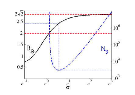
Figure 2: Violation of the sequential CHSH test. Solid line: BSsubscript𝐡𝑆B_{S} as a function of the measurements inaccuracy σ≑Δ​q​(t=0)πœŽΞ”π‘žπ‘‘0\sigma\equiv\Delta q(t=0). BS>2subscript𝐡𝑆2B_{S}>2 for Οƒ>[βˆ’2​ln⁑(23/4βˆ’1)]βˆ’1∼1.1425𝜎superscriptdelimited-[]2superscript23411similar-to1.1425\sigma>\sqrt{[-2\ln(2^{3/4}-1)]^{-1}}\sim 1.1425. Note that precise sequential measurements satisfy CHSH inequality. Broken line: ensemble size N3​(Οƒ)subscript𝑁3𝜎N_{3}(\sigma) that manifests violation with three standard deviations. BS∼2.43similar-tosubscript𝐡𝑆2.43B_{S}\sim 2.43 corresponds to the minimal ensemble size N3=3088subscript𝑁33088N_{3}=3088. For comparison, the regular non-sequential precise setting requires N3=105subscript𝑁3105N_{3}=105.
Refer to caption
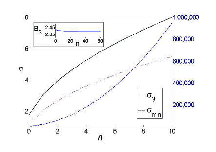
Figure 3: Simultaneous violation of several CHSH tests. The parties perform n𝑛n CHSH experiments before starting the current CHSH sequence. BS>2subscript𝐡𝑆2B_{S}>2 for Οƒ>Οƒmin𝜎subscript𝜎min\sigma>\sigma_{\mbox{min}} (dotted line), where Οƒmin=23/4​nsubscript𝜎minsuperscript234𝑛\sigma_{\mbox{min}}=2^{3/4}\sqrt{n} (for large enough n𝑛n). Also shown is the minimal value of N3subscript𝑁3N_{3} (broken line) and the corresponding Οƒ3subscript𝜎3\sigma_{3} (solid line) which manifests violation with 3 standard deviations. N3subscript𝑁3N_{3} scales quadratically with n𝑛n. Inset: Expected violation given Οƒ3subscript𝜎3\sigma_{3}. BS​(n)subscript𝐡𝑆𝑛B_{S}(n) decreases slowly with n𝑛n where BS∼2.4similar-tosubscript𝐡𝑆2.4B_{S}\sim 2.4.

The strict limit of weak measurements requires an infinite ensemble, which is not practical. However, violation can be observed using a finite ensemble, and finite measurement apparatus inaccuracy σ≑Δ​q​(t=0)πœŽΞ”π‘žπ‘‘0\sigma\equiv\Delta q(t=0), as illustrated in fig. 2. In fact, we find that BS>2subscript𝐡𝑆2B_{S}>2 for relatively mild value of ΟƒβˆΌ1.15similar-to𝜎1.15\sigma\sim 1.15. As the inaccuracy increases BSβ†’2​2β†’subscript𝐡𝑆22B_{S}\to 2\sqrt{2}. Also shown is the required ensemble size N3subscript𝑁3N_{3} by which violation is manifested with three standard deviations. The minimal ensemble is about thirty times larger the one required to manifest B>2𝐡2B>2 in the usual setting.

Furthermore, simultaneous violation of (possibly different) Bell inequalities can be observed using the same ensemble. For example, assume that the two parties perform n𝑛n CHSH sequences on each pair of the ensemble with a fixed inaccuracy ΟƒπœŽ\sigma before starting the current CHSH test. In fig. 3 we show the minimal ensemble size N3subscript𝑁3N_{3} and the corresponding inaccuracy Οƒ3subscript𝜎3\sigma_{3} by which violation is manifested.

We proceed by quantifying the required inaccuracy of the measurements as depicted in figures 2 and 3. By explicitly expanding the joint state of the system and the measurement apparatuses it can be shown that E​(q1A​q1B)=12𝐸subscriptsuperscriptπ‘žπ΄1subscriptsuperscriptπ‘žπ΅112E(q^{A}_{1}q^{B}_{1})=\frac{1}{\sqrt{2}}, E​(q2A​q1B)=E​(q1A​q2B)=y2𝐸subscriptsuperscriptπ‘žπ΄2subscriptsuperscriptπ‘žπ΅1𝐸subscriptsuperscriptπ‘žπ΄1subscriptsuperscriptπ‘žπ΅2𝑦2E(q^{A}_{2}q^{B}_{1})=E(q^{A}_{1}q^{B}_{2})=\frac{y}{\sqrt{2}} and E​(q2A​q2B)=y22𝐸subscriptsuperscriptπ‘žπ΄2subscriptsuperscriptπ‘žπ΅2superscript𝑦22E(q^{A}_{2}q^{B}_{2})=\frac{y^{2}}{\sqrt{2}}, where y≑eβˆ’Ο΅/2=eβˆ’12​σ2𝑦superscript𝑒italic-Ο΅2superscript𝑒12superscript𝜎2y\equiv e^{-\epsilon/2}=e^{-\frac{1}{2\sigma^{2}}}. For example, the mutual state of the system and the measuring devices after party A𝐴A measures both ΟƒxAsubscriptsuperscript𝜎𝐴π‘₯\sigma^{A}_{x} and then ΟƒzAsubscriptsuperscriptπœŽπ΄π‘§\sigma^{A}_{z} and party B𝐡B measures σπ/4BsubscriptsuperscriptπœŽπ΅πœ‹4\sigma^{B}_{\pi/4} is

|↑z↑π/4βŸ©Ο•(q2Aβˆ’1)Ο•(q1Bβˆ’1)(Ξ±Ο•(q1Aβˆ’1)βˆ’Ξ²(q1A+1))+|↓z↑π/4βŸ©Ο•(q2A+1)Ο•(q1Bβˆ’1)(Ξ±Ο•(q1Aβˆ’1)+Ξ²(q1A+1))+|↑z↓π/4βŸ©Ο•(q2Aβˆ’1)Ο•(q1B+1)(Ξ²Ο•(q1Aβˆ’1)+Ξ±(q1A+1))+|↓z↓π/4βŸ©Ο•(q2A+1)Ο•(q1B+1)(Ξ²Ο•(q1Aβˆ’1)βˆ’Ξ±(q1A+1)),\begin{split}&|\uparrow_{z}\uparrow_{\pi/4}\rangle\phi(q^{A}_{2}\!-\!1)\phi(q^{B}_{1}\!-\!1)\big{(}\alpha\phi(q^{A}_{1}\!-\!1)-\beta(q^{A}_{1}\!+\!1)\big{)}\\ +&|\downarrow_{z}\uparrow_{\pi/4}\rangle\phi(q^{A}_{2}\!+\!1)\phi(q^{B}_{1}\!-\!1)\big{(}\alpha\phi(q^{A}_{1}\!-\!1)+\beta(q^{A}_{1}\!+\!1)\big{)}\\ +&|\uparrow_{z}\downarrow_{\pi/4}\rangle\phi(q^{A}_{2}\!-\!1)\phi(q^{B}_{1}\!+\!1)\big{(}\beta\phi(q^{A}_{1}\!-\!1)+\alpha(q^{A}_{1}\!+\!1)\big{)}\\ +&|\downarrow_{z}\downarrow_{\pi/4}\rangle\phi(q^{A}_{2}\!+\!1)\phi(q^{B}_{1}\!+\!1)\big{(}\beta\phi(q^{A}_{1}\!-\!1)-\alpha(q^{A}_{1}\!+\!1)\big{)},\end{split}

where Ξ±=12​2​[cos⁑(Ο€/8)+sin⁑(Ο€/8)]𝛼122delimited-[]πœ‹8πœ‹8\alpha=\frac{1}{2\sqrt{2}}[\cos(\pi/8)+\sin(\pi/8)], Ξ²=12​2​[sin⁑(Ο€/8)βˆ’cos⁑(Ο€/8)]𝛽122delimited-[]πœ‹8πœ‹8\beta=\frac{1}{2\sqrt{2}}[\sin(\pi/8)-\cos(\pi/8)]. By tracing out the system and q1Asuperscriptsubscriptπ‘ž1𝐴q_{1}^{A}, one can compute E​(q2A​q1B)𝐸superscriptsubscriptπ‘ž2𝐴superscriptsubscriptπ‘ž1𝐡E(q_{2}^{A}q_{1}^{B}) given above. Therefore BS=12​(1+y)2subscript𝐡𝑆12superscript1𝑦2B_{S}=\frac{1}{\sqrt{2}}(1+y)^{2}, where BSsubscript𝐡𝑆B_{S} denotes the sequential setting.

By the central limit theorem the size of the ensemble which is required to manifest violation of Bell inequality with z𝑧z standard deviations is determined by

z​V​(B)N3<Bβˆ’2,𝑧𝑉𝐡subscript𝑁3𝐡2z\sqrt{\frac{V(B)}{N_{3}}}<B-2, (14)

where V​(B)𝑉𝐡V(B) is the variance of B𝐡B. In the regular non-sequential setting B𝐡B is the sum of four independent variables V​(B)β‰‘βˆ‘i,jV​(qiA​qjB)=4​(1+Οƒ2)2βˆ’2𝑉𝐡subscript𝑖𝑗𝑉subscriptsuperscriptπ‘žπ΄π‘–subscriptsuperscriptπ‘žπ΅π‘—4superscript1superscript𝜎222V(B)\equiv\sum_{i,j}V(q^{A}_{i}q^{B}_{j})=4(1+\sigma^{2})^{2}-2. In case of sequential measurements the experiments are dependent, thus V​(BS)β‰‘βˆ‘i,j,k,lC​V​(qiA​qjB,qkA​qlB)𝑉subscript𝐡𝑆subscriptπ‘–π‘—π‘˜π‘™πΆπ‘‰subscriptsuperscriptπ‘žπ΄π‘–subscriptsuperscriptπ‘žπ΅π‘—subscriptsuperscriptπ‘žπ΄π‘˜subscriptsuperscriptπ‘žπ΅π‘™V(B_{S})\equiv\sum_{i,j,k,l}CV(q^{A}_{i}q^{B}_{j},q^{A}_{k}q^{B}_{l}), where C​V​(x,y)=E​(x​y)βˆ’E​(x)​E​(y)𝐢𝑉π‘₯𝑦𝐸π‘₯𝑦𝐸π‘₯𝐸𝑦CV(x,y)=E(xy)-E(x)E(y) is the mutual covariance. By a straightforward computation it can be shown that for iβ‰ kπ‘–π‘˜i\neq k and jβ‰ l𝑗𝑙j\neq l, C​V​(qiA​ajB,qiA​alB)=C​V​(qiA​qjB,qkA​qlB)=0𝐢𝑉subscriptsuperscriptπ‘žπ΄π‘–subscriptsuperscriptπ‘Žπ΅π‘—subscriptsuperscriptπ‘žπ΄π‘–subscriptsuperscriptπ‘Žπ΅π‘™πΆπ‘‰subscriptsuperscriptπ‘žπ΄π‘–subscriptsuperscriptπ‘žπ΅π‘—subscriptsuperscriptπ‘žπ΄π‘˜subscriptsuperscriptπ‘žπ΅π‘™0CV(q^{A}_{i}a^{B}_{j},q^{A}_{i}a^{B}_{l})=CV(q^{A}_{i}q^{B}_{j},q^{A}_{k}q^{B}_{l})=0, and V​(qiA​qjB)=(1+Οƒ2)2𝑉subscriptsuperscriptπ‘žπ΄π‘–subscriptsuperscriptπ‘žπ΅π‘—superscript1superscript𝜎22V(q^{A}_{i}q^{B}_{j})=(1+\sigma^{2})^{2}. Therefore V​(BS)=4​(1+Οƒ2)2βˆ’12​(1+y)4𝑉subscript𝐡𝑆4superscript1superscript𝜎2212superscript1𝑦4V(B_{S})=4(1+\sigma^{2})^{2}-\frac{1}{2}(1+y)^{4}. These results are illustrated in fig. 2.

Now assume that the two parties perform n𝑛n CHSH sequences before starting the current CHSH experiment, where the i𝑖ith observable of each party is maximally non-commuting with the iβˆ’1𝑖1i-1 one for any i𝑖i. Then it can be shown that

BS​(n)=y2​n2​(1+y)2subscript𝐡𝑆𝑛superscript𝑦2𝑛2superscript1𝑦2B_{S}(n)=\frac{y^{2n}}{\sqrt{2}}(1+y)^{2} (15)

and V​(BS​(n))=4​(1+Οƒ2)2βˆ’y2​n2​(1+y)4𝑉subscript𝐡𝑆𝑛4superscript1superscript𝜎22superscript𝑦2𝑛2superscript1𝑦4V\big{(}B_{S}(n)\big{)}=4(1+\sigma^{2})^{2}-\frac{y^{2n}}{2}(1+y)^{4}. These results are illustrated in fig. 3. It can be numerically shown that Eq. (15) yields a typical value for randomly chosen n=2​m𝑛2π‘šn=2m measurements.

V Maximal violation of Leggett-Garg inequalities

Our suggestion to manifest violation of Bell inequalities is related to the time inequalities first suggested by Leggett and Garg (LG) leggett . LG discuss measurements on a local system which are performed at different times. They analyze the scenario in which at each cycle the experimentalist chooses two out of m>2π‘š2m>2 measurements and compute their mutual expectation value. Given a realistic model and non-demolition measurements, correlations satisfy the LG inequalities, which have a similar structure to Bell inequalities. Interestingly, it was shown that quantum theory violates the LG inequalities using weak measurements mizel ; jordan1 ; jordan even if all observables are measured on each member of the ensemble. In this setting precise measurements do not violate LG inequalities by definition. The addition of noise, however, distinguishes models incorporating LG assumptions from quantum theory, since non-demolition measurements imply that the noise and the measured observable are independent mizel . This is violated in quantum theory even though the effect of weak measurements on the system is small. An immediate consequence of Eq. (4) is that LG inequalities are maximally violated by quantum theory in the limit of weak measurements. Note that the realism assumption is crucial since one can write a joint probability distribution to the pointers of weak measurements, which do not correspond to Β±1plus-or-minus1\pm 1 values.

VI Conclusions

We propose a new approach to test quantum nonlocality, in which all observables are measured on each system without the need to select randomly a single observable. By enlarging the sequence of measurements it is also possible to manifest a simultaneous violation of more than one Bell inequality. Our proposal can be demonstrated in all systems in which both Bell state preparation and sequential weak measurements are realizable, for example atomic physics devices ion , photons amplify ; photon , and solid-state qubits NP .

Acknowledgements.
We thank P. Skrzypczyk, N. Klinghoffer, J. Kupferman and G. Ben-Porath for helpful discussions. This work has been supported by the Israel Science Foundation grant numbers 784/06, 920/09.

References

  • (1) Bell JS (1964) On the Einstein-Podolsky-Rosen paradox. Physics (Long Island City, N.Y.) 1:195-200.
  • (2) Aspect A, Dalibard J, Roger G (1982) Experimental test of Bell’s inequalities using time-varying analyzers. Phys. Rev. Lett. 49:1804-1807.
  • (3) Weihs G, Jennewein T, Simon C, Weinfurter H, Zeilinger A (1998) Violation of Bell’s Inequality under Strict Einstein Locality Conditions. Phys. Rev. Lett. 81:5039-5043.
  • (4) Clauser JF, Horne MA, Shimony A, Holt RA (1969) Proposed Experiment to Test Local Hidden-Variable Theories. Phys. Rev. Lett. 23:880-884.
  • (5) Cirel’son BS (1980) Quantum generalizations of Bell’s inequality. Lett. Math. Phys. 4:93-100.
  • (6) von Neumann J (1955) in Mathematical Foundations of Quantum Mechanics (Princeton University Press, Princeton).
  • (7) Aharonov Y, Albert DZ, Casher A, Vaidman L (1987) Surprising quantum effects. Phys. Lett. A 124:199-203.
  • (8) Leggett AJ, Garg A (1985) Quantum mechanics versus macroscopic realism: Is the flux there when nobody looks? Phys. Rev. Lett. 54:857-860.
  • (9) Korotkov AN, Averin DV (2001) Continuous weak measurement of quantum coherent oscillations. Phys. Rev. B 64:165310-165314.
  • (10) Resch KJ, Steinberg AM (2004) Extracting Joint Weak Values with Local, Single-Particle Measurements. Phys. Rev. Lett. 92:130402-130405.
  • (11) Mitchison G, Jozsa R and Popescu S (2007) Sequential weak measurement. Phys. Rev. A 76:062105-062113.
  • (12) Lundeen JS, Steinberg AM (2009) Experimental Joint Weak Measurement on a Photon Pair as a Probe of Hardy s Paradox. Phys. Rev. Lett. 102:020404-020407.
  • (13) Johansen LM, Mello PA (2008) Quantum mechanics of successive measurements with arbitrary meter coupling. Physics Lett. A 372:5760-5764.
  • (14) Ruskov R, Korotkov AN, Mizel A (2006) Signatures of quantum behavior in single-qubit weak measurements. Phys. Rev. Lett. 96:200404-200407.
  • (15) Jordan AN, Korotkov AN, BΓΌttiker M (2006) Leggett-Garg inequality with a kicked quantum pump. Phys. Rev. Lett. 97:026805-026808.
  • (16) Williams NS, Jordan AN (2008) Weak Values and the Leggett-Garg Inequality in Solid-State Qubits. Phys. Rev. Lett. 100:026804-026807.
  • (17) MΓΈlmer K (2001) Counterfactual statements and weak measurements: an experimental proposal. Phys. Lett. A 292:151-155.
  • (18) Hosten O, Kwiat P (2008) Observation of the Spin Hall Effect of Light via Weak Measurements. Science 319:787-790.
  • (19) Goggin ME et. al. (2009) Violation of the Leggett-Garg inequality with weak measurements of photons. e-print arXiv: 0907.1679.
  • (20) Palacios-Laloy A. et. al. (2010) Experimental violation of a Bell’s inequality in time with weak measurement. Nature Phys. 6:442-447.