Detection of GW bursts with chirplet-like template families
Abstract
Gravitational Wave (GW) burst detection algorithms typically rely on the hypothesis that the burst signal is “locally stationary”, that is it changes slowly with frequency. Under this assumption, the signal can be decomposed into a small number of wavelets with constant frequency. This justifies the use of a family of sine-Gaussian wavelets in the Omega pipeline, one of the algorithms used in LIGO-Virgo burst searches. However there are plausible scenarios where the burst frequency evolves rapidly, such as in the merger phase of a binary black hole and/or neutron star coalescence. In those cases, the local stationarity of sine-Gaussians induces performance losses, due to the mismatch between the template and the actual signal. We propose an extension of the Omega pipeline based on chirplet-like templates. Chirplets incorporate an additional parameter, the chirp rate, to control the frequency variation. In this paper, we show that the Omega pipeline can easily be extended to include a chirplet template bank. We illustrate the method on a simulated data set, with a family of phenomenological binary black-hole coalescence waveforms embedded into Gaussian LIGO/Virgo–like noise. Chirplet-like templates result in an enhancement of the measured signal-to-noise ratio.
1 Motivations
Current searches for gravitational wave transients in LIGO-Virgo data focus on two signal classes: short unmodelled bursts and longer quasi-periodic signals from inspiralling black hole and/or neutron star binaries as predicted by post-Newtonian approximations. To account for intermediate scenarios, we consider “chirping burst” GW target signals that exhibit characteristics from both the above categories: a short duration and a “sweeping” frequency.
We propose here an extension of the Omega pipeline [3] (originally known as pipeline) that searches for chirping bursts. The Omega pipeline projects the data over a family of sine-Gaussian wavelets with fixed frequency. The idea is to replace these templates by frequency varying waveforms, referred to as chirplets.
In this paper, we first define chirplets and the related chirplet transform. We discuss the implementation of the chirplet transform and its insertion into the Omega pipeline, with attention to how the chirplet template bank is built. Finally, we present a few examples using simulated data.
2 From wavelets to chirplets
2.1 Definition of chirplets
Chirplets are defined in the time domain as:
| (1) |
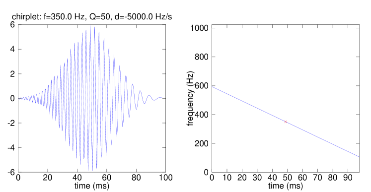
with , a normalization factor ensuring that . and are the center time and frequency, respectively and is the dimensionless quality factor. See in Fig. 1 for an example of a chirplet.
The main difference from a sine-Gaussian wavelets is the chirp rate, an additional term in the phase denoted that changes the chirplet frequency linearly in time as . The chirp rate controls the slope of the frequency evolution. When , we retrieve standard sine-Gaussians. Chirplets are thus associated with a four-dimensional parameter space instead of three for sine-Gaussians. In the sequel, we will concatenate all those parameters into a descriptor .
2.2 Chirplet transform
The chirplet transform is obtained by correlating the data with the chirplets defined in the previous section. In the frequency domain, it reads:
| (2) |
where and denotes the Fourier transform of the (whitened) data stream and chirplet with descriptor resp.
The chirplet Fourier transform can be expressed as
| (3) |
where is written in terms of a “complex-valued” quality factor where with the chirplet duration111By definition, . .
3 Building template banks with chirplets
By varying the chirplet parameters, we obtain a continuous signal space. In this space, we need to select a finite-size family of representatives which will be used to analyze the data. The coverage of the chirplet space has to meet two conflicting goals i.e., satisfy a worst case mismatch with a minimum number of templates. We adopt the method proposed in [4, 3] which consists of sampling the space with equi-spaced templates using the intrinsic metric deduced from the mismatch between two neighboring templates with a small discrepancy in their parameters. The metric results from the second-order expansion of the mismatch when and leads to222This calculation assumes that the detector noise has a flat spectrum. Contrarily to the sine-Gaussian case, this approximation has significant effect since the chirplet frequency varies across the detector bandwidth.:
| (4) |
There are several differences and additional terms from the sine-Gaussian metric, due to the non-zero chirping rate. Along the time axis and for small , the sampling step is finer than that of the sine-Gaussian case . We note also that the sampling step along the chirping rate axis scales with . We thus expect to get many chirplets in the low-frequency band and for large values of .
The chirplet space equipped with the above metric (off-diagonal terms being neglected for simplicity [3]) can be discretized by a cubic lattice with templates placed at the vertices. The worst case occurs when the real signal is farther apart from all vertices, at the center of the cube. Let us denote , this worst-case distance, which corresponds to the half-length of the cube diagonal and assign a maximum value that we can tolerate. Since we are in a four-dimensional space, the length of the cube edge is equal to that of its half-diagonal. Therefore, we must have . The discretization along each axis of the parameter space which results directly from this condition ensures that for any with the closest vertex of the lattice. In the following, we set the maximum mismatch to the value typically used when applying standard Omega. Fig. 2 shows an example of a chirplet template bank resulting from this template placement scheme.
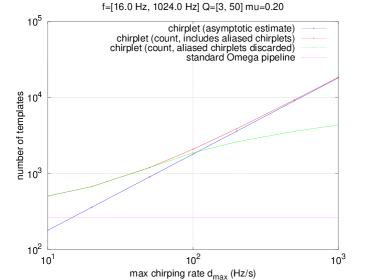
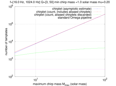
In Fig. 3, we apply the same scheme in two different settings. In both cases we computed the number of templates necessary to cover the signal space in the sine-Gaussian (standard Omega) and chirplet (chirpletized Omega) cases. This computation is done at a fixed time . We compare the result to the estimate given by the ratio of the whole space volume (where and denotes the metric in Eq. (4) without the components associated to the time axis) to the size of a cubic element of the lattice. We find333This result is valid both when neglecting or retaining the off-diagonal terms of the metric. The scaling is actually exact when the off-diagonal terms are included and valid to a good approximation when in the other case.:
| (5) |
where we assume that for each coordinate the lower boundaries (min) are much smaller than the higher boundaries (max).
It is important to note that both the count and estimate are obtained assuming an infinite bandwidth. Since the data are sampled, we are restricted to a limited Nyquist frequency. Chirplets with frequency exceeding this limits are aliased and have to be discarded. Fig. 3 also show the number of non-aliased chirplets. This number is about a factor of 10 larger than the number of sine-Gaussians required to cover the entire parameter space.
Two comments can be made at this point: the larger number of templates indicate that with chirplets, we define and explore a much larger signal space than with sine-Gaussians (we investigate this question further in Sec. 5). As the computing cost scales approximately linearly with the number of templates, analyzing the data with chirplets requires with a ten-fold increase in computing resources (a factor that will be rapidly absorbed by the exponential growth of computing power).

4 From “standard” to “chirpletized” Omega
In this session we discuss other aspects of the analysis pipeline, in addition to the implementation of the chirplet template bank.
4.1 Filtering
The modulus of in Eq. (3) is a Gaussian function as in the sine-Gaussian case. This allows the use of the same filtering scheme as in the standard Omega pipeline to generate the chirplet transform. The Omega scheme [3] operates in the frequency domain following Eq. (2). It consists in multiplying the Fourier transform of the data, computed with the FFT algorithm, with that of the templates and take the inverse Fourier transform of the product. Omega uses a bi-square frequency window that approximates the Gaussian shape. The compact support of the bi-square window prevents aliasing.
This scheme can be applied to the chirplet case with two differences. First, the template is now complex, thus we need to multiply the data spectrum both in modulus and phase. Second, the template bandwidth now results from the quadratic sum of two components, one due to the finite size of the chirplet and the other due to its sweeping frequency , where is the chirplet duration (defined above). According to [3], the width of the bi-square window should be set to the chirplet frequency bandwidth rescaled by a factor of .
4.2 Pre- and post-processing
In this paper we focus on a single-detector network, where most of the pre- and post-processing can be adopted from the standard Omega pipeline. Pre-processing consists of whitening the input data stream. Post-processing consists of selecting among the chirplets with partial time and frequency overlap to the one with maximum correlation with the data. Each chirplet is associated with a time-frequency tile, defined by where and are the chirplet duration and bandwidth, respectively. Two chirplets overlap if their time-frequency tiles overlap.
5 Performances of Chirpletized Omega
In this section we present a comparison between the standard version of the Omega pipeline, which uses sine-Gaussian wavelets, and its chirpletized version. We configure the pipelines with identical values for the parameters they have in common (frequency and Q range and maximum mismatch). We identify cases where we can expect advantages from analyzing the data with chirplets.
5.1 Analyzing chirplets with sine-Gaussians
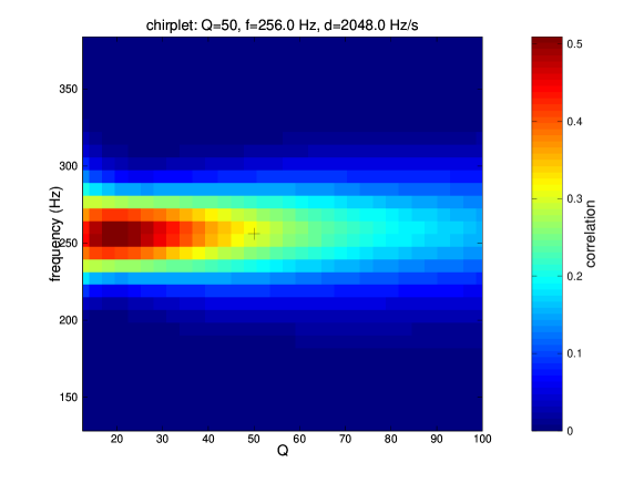
The signal space associated with sine-Gaussians is contained in the larger space associated with chirplets. We estimate the signal-to-noise ratio (SNR) loss occurring when analyzing a chirplet by correlating this signal against a sine-Gaussian template bank. The chirplet parameters have been set to , Hz and Hz/s. Those parameters correspond to observable physical signals in the LIGO/Virgo frequency band (for instance, the selected chirping rate is approximately that of an inspiralling binary chirp with total mass – assuming equal masses – at Hz according to the Newtonian model). Fig. 4 presents the result of this analysis. Consistently to the metric estimate, the loss is in the present case. Note also that the maximum correlation is shifted to lower which may lead to a possible bias in the estimation of this parameter.
5.2 Analyzing inspiralling binary chirps with chirplets
One case study —
As an illustration, we show here results from chirpletized Omega on simulated Gaussian noise, colored with the spectral characteristics of LIGO/Virgo noise with simulated gravitational wave signals. The signal we consider here results from the phenomenological approximation introduced in [2] of the coalescing binary black-hole chirp signals and includes the inspiral, merger and ringdown parts of the coalescence.
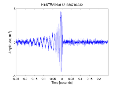
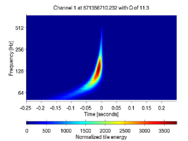
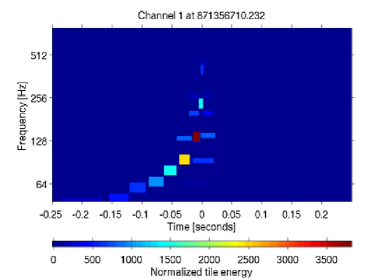
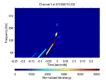
In Fig. 5, we compare the results from the standard and chirpletized Omega pipelines obtained for a black-hole binary chirp embedded in simulated Gaussian noise at large SNR. Chirplets with a positive slope are preferred to sine-Gaussian with constant frequency: the correlation of the most significative chirplet is, in this example, larger than the most significative sine-Gaussian. Work is currently in progress to understand how the background in chirpletized Omega is different from standard Omega. Preliminary studies in Gaussian noise suggest that the background rates are comparable, so that we can expect an increase of in distance reach by using chirplets.
Note that the chirplet slope provides indication of the frequency evolution of the observed signal and thus may be very useful in the a posteriori interpretation of an event.
Systematic study —
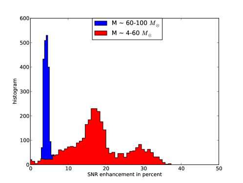
We also performed a more systematic comparison over a population of inspiralling binaries. We considered a total of 5500 binaries with equal mass components. The total mass is extracted from a flat distribution in the range. The signal amplitudes are scaled so that the SNR is distributed over an interval ranging from to .
We obtain an estimate of the injected SNR from the amplitude of the most significant template. In the ideal case where signal and template are identical, the estimate equals the injected value. In Fig. 6, we show the relative difference of the SNR estimated by chirpletized Omega and standard Omega. Chirpletized Omega estimates a higher SNR across the mass range. However, there are two regimes: for the high-mass range , the SNR improvement is small () while it is more pronounced () for the low-mass range . The improvement may go upto for .
Generally speaking, the spectrum of the GW chirp is shifted toward low frequencies when the binary mass increases. The frequency associated with the innermost stable circular orbit (ISCO), which corresponds to the transition between inspiral and merger phase of the coalescence, is below 70 Hz for masses . In this condition, the chirp phase of the waveform with a spectral content at frequencies below ISCO is outside the detector sensitive band444This statement is valid for the LIGO detector noise curve which was used for the systematic study. The mass cut-off is higher for the Virgo detector as its sensitive band extends to lower frequencies. and thus does not contribute significantly to the SNR. Sine-Gaussian waveform provides a good enough fit of the remaining few waveform cycles associated with the merger and ringdown parts of the coalescence. This explains the two regimes in Fig. 6.
 |
 |
 |
 |
6 Status and future plans
We introduced a new chirplet-based extension of the Omega pipeline. We show preliminary results using coalescing binary mergers waveforms. Versatility (robustness to signal model uncertainty) and algorithmic simplicity are two advantages of this methodology when compared to more standard approaches for the detection of such waveforms.
The single-detector network search code is ready and it can be downloaded [1] and used to produce chirpletized Omega scans similar to the one we show in Fig. 5.
We continue to study the response of the code to real noise and we aim at a complete, operating pipeline using chirplets as templates, and new clustering strategies tailored to these templates, as well as a multi-detector network strategy.
References
References
- [1] https://geco.phys.columbia.edu/omega/browser/branches/chirplet.
- [2] P. Ajith et al. ’Complete’ gravitational waveforms for black-hole binaries with non-precessing spins, 2009. arXiv:0909.2867.
- [3] S. K. Chatterji. The search for gravitational-wave bursts in data from the second LIGO science run. PhD thesis, MIT Dept. of Physics, 2005.
- [4] B. J. Owen and B. S. Sathyaprakash. Matched filtering of gravitational waves from inspiraling compact binaries: Computational cost and template placement. Phys. Rev., D60:022002, 1999. gr-qc/9808076.
Acknowlegments
We are grateful to the LIGO Scientific Collaboration for the use of its algorithm library available at https://www.lsc-group.phys.uwm.edu/daswg/projects/lalapps.html. This work is supported in part by NSF grant PHY-0653550. M. Miele is supported by an ERASMUS fellowhip from the University of Sannio at Benevento (Italy).