Trial factors for the look elsewhere effect in high energy physics

Abstract

When searching for a new resonance somewhere in a possible mass range, the significance of observing a local excess of events must take into account the probability of observing such an excess anywhere in the range. This is the so called “look elsewhere effect”. The effect can be quantified in terms of a trial factor, which is the ratio between the probability of observing the excess at some fixed mass point, to the probability of observing it anywhere in the range. We propose a simple and fast procedure for estimating the trial factor, based on earlier results by Davies. We show that asymptotically, the trial factor grows linearly with the (fixed mass) significance.

1 Introduction

The statistical significance that is associated to the observation of new phenomena is usually expressed using a p-value, that is, the probability that a similar or more extreme effect would be seen when the signal does not exist (a situation usually referred to as the null or background-only hypothesis). It is often the case that one does not a priori know where the signal will appear within some possible range. In that case, the significance calculation must take into account the fact that an excess of events anywhere in the range could equally be considered as a signal. This is known as the “look elsewhere effect” lyons luc . In the statistical literature this situation is usually referred to as an hypothesis test when a nuisance parameter is present only under the alternative, for which the standard regularity conditions do not apply. The problem is however closely related to that of a level crossings of a stochastic process, which has been studied extensively and for which many relevant results exist davis77 ,davis87 . In particular davis87 provides an upper bound on the tail probability of the maximum of a chi-squared process, which can therefore be applied to cases when the test statistic is the profile likelihood ratio and the large-sample distribution at a fixed point given by Wilks’ theorem wilks holds.

Of course, a straightforward way of quantifying the look-elsewhere effect may be simply running many Monte-Carlo simulations of background only experiments, and finding for each one the largest fluctuation that resembles a signal. Examples for such an approach can be found e.g. in examples . While this procedure is simple and gives the correct answer, it is also time and CPU consuming, as one would have to repeat it $\mathcal{O}(10^{7})$ times to get the p-value corresponding to a $5\sigma$ significance. Approximations based on large sample limits such as davis87 can therefore be valuable.

To make the discussion concrete, let us first describe a typical example of a ‘mass bump’ search. The statistical model in this case consists of a background distribution $b$, and a signal distribution $s(m)$ with an unknown location parameter $m$ (corresponding to the mass of a resonance). We introduce a signal strength parameter $\mu$, such that the model is given by $\mu s(m)+b$, and we test $H_{0}:\mu=0$ against the alternative, $\mu>0$ . Both $s$ and $b$ may depend on additional nuisance parameters which are omitted from the notation. The mass $m$ is another nuisance parameter, but it does not exist under $H_{0}$ since $b$ does not depend on $m$. The testing problem has therefore a nuisance parameter that is present only under the alternative. When searching for a resonance that can appear anywhere in the range, one will look for the largest excess of events above the background. More precisely, if $q(m)$ is a test statistic for a fixed mass, and large values of $q(m)$ indicate decreasing compatibility with the null hypothesis, then the test statistic of the entire range would be $q(\hat{m})=\displaystyle\max_{m}[q(m)]$. The problem is therefore in assessing the tail probability (p-value) of the maximum of $q(m)$ over the search range.

In section 2 we review the main result of davis87 and its application to the present case. We propose a practical procedure for estimating the p-value, which we then demonstrate with a toy model simulation in section 3.

2 Tail probabilities of the likelihood ratio test statistic

Suppose that a signal hypothesis depends on a nuisance parameter $\theta$ that does not exist under the null. We denote by $q(\theta)$ the profile likelihood test statistic for some fixed $\theta$ and we assume that it follows a $\chi^{2}$ distribution with $s$ degrees of freedom, as would be the case in the large sample limit when Wilks’ theorem holds. We are interested in the tail probability of the maximum of $q(\theta)$ over $\theta$, which we denote by $q(\hat{\theta})$. As shown in davis87 , this is bounded by:

$$P(q(\hat{\theta})>c)\leqslant P(\chi^{2}_{s}>c)+\langle N(c)\rangle$$ (1)

where $N(c)$ is the number of ‘upcrossings’ of the level $c$ by the process $q(\theta)$, with an expectation that is given by davis87 :

$$\langle N(c)\rangle=\frac{c^{(s-1)/2}e^{-c/2}}{\sqrt{\pi}2^{s/2}\Gamma(s/2+1/2)}\int_{L}^{U}C(\theta)d\theta$$ (2)

Where $[L,U]$ is the range of possible values of $\theta$, and $C(\theta)$ is some function that depends on the details of the statistical model. To have the maximum of $q(\theta)$ above the level $c$ means that either the value at the lower threshold $q(L)$ is larger than $c$, or that there is at least one upcrossing, hence the two terms in (1). Note that the bound is expected to become an equality for large values of $c$, as the expected number of upcrossings will be dominated by the probability of one upcrossing, that is when $\langle N(c)\rangle\ll 1$.

The function $C(\theta)$ can in general be difficult to calculate. Instead, we propose to estimate $\langle N(c_{0})\rangle$ at some low reference level $c_{0}$ by simply counting the number of upcrossings in a small set of background-only Monte Carlo simulations. Eq. (1) then becomes

$$P(q(\hat{\theta})>c)\leqslant P(\chi^{2}_{s}>c)+\langle N(c_{0})\rangle(\frac{c}{c_{0}})^{(s-1)/2}e^{-(c-c_{0})/2}$$ (3)

and so once $\langle N(c_{0})\rangle$ is determined, the p-value of a given observation and the corresponding significance are readily obtained.

Naturally, one would like to choose the reference level $c_{0}$ in a way that will minimize the resulting uncertainty on the bound. From (3), it can be seen that the statistical uncertainty is proportional to $\sigma_{N}/\langle N\rangle$ where $\sigma_{N}$ is the standard deviation of $N$. As long as the the distribution of $N$ is ‘well behaved’ in the sense that the relative uncertainty decreases with increasing $\langle N\rangle$, then the optimal choice of $c_{0}$ would be that which maximizes the expected number of upcrossings (2), that is $c_{0}=s-1$. Note that in the case $s=1$, the maximal number of upcrossings occurs at $c_{0}\to 0$, however the ability to reliably estimate $\langle N(c_{0})\rangle$ at very low levels depends on the numerical resolution at which $q(\theta)$ is calculated. In this case, one should therefore aim at having $c_{0}$ as low as possible but still significantly larger than the numerical resolution of $q(\theta)$, and the typical distance between upcrossings should be kept significantly larger than the $\theta$ resolution. In the example considered in the following section $c_{0}=0.5$ satisfies those conditions and proves to be a good choice.

It is further interesting to note that the dependence of $\langle N(c)\rangle$ on $c$ in (2), is the same as the asymptotic form of the cumulative distribution of a $\chi^{2}$ variable with $s+1$ degrees of freedom,

$$P(\chi^{2}_{s+1}>c)\xrightarrow[c\to\infty]{}\frac{c^{\frac{1}{2}(s+1)-1}e^{-c/2}}{2^{\frac{1}{2}(s+1)-1}\mathrm{\Gamma}((s+1)/2)}$$ (4)

allowing us to write, for large $c$ ($c\gg s$),

$$P(q(\hat{\theta})>c)\approx P(\chi^{2}_{s}>c)+\mathcal{N}P(\chi^{2}_{s+1}>c)$$ (5)

where

$$\mathcal{N}=\frac{1}{\sqrt{2\pi}}\int_{L}^{U}C(\theta)d\theta$$ (6)

And the bound has been replaced by a ‘$\approx$’ sign since we are dealing with the large $c$ limit. The probability described by eq. (5) has a natural interpretation. It is the same as one would have for a random variable that is the maximal of $n$ independent $\chi^{2}_{s+1}$ variates and one $\chi^{2}_{s}$ variate, with $E[n]=\mathcal{N}$. That is, if

$$y=\max[x_{0},x_{1}...x_{n}]$$ (7)

and

$x_{0}\sim\chi^{2}_{s}$,

$x_{i}\sim\chi^{2}_{s+1}$

$i=1...n$,

$E[n]=\mathcal{N}$

then the tail probability $P(y>c)$ for large $c$ is given by the right hand side of (5).

Intuitively, this suggests that we can view the range of $\theta$ as being composed of several (on average $\mathcal{N}$) independent regions , where in each one the likelihood fit involves an extra degree of freedom due to the variable mass, leading to a $\chi^{2}_{s+1}$ distribution. The $\chi^{2}_{s}$ term accounts for the possibility of having a local maximum on the edge of the allowed region (assuming, from symmetry reasons, that each edge has a probability $1/2$ of being a local maximum). The number $\mathcal{N}$ can therefore be interpreted as an ‘effective number’ of independent search regions.

We remark that exactly such an intuitive reasoning was employed by Quayle quayle as a conjecture for the distribution of $q(\hat{\theta})$. It was found that the distribution of a random variable defined according to (7) reproduces, to a good approximation, that of $q(\hat{\theta})$, and that the agreement is better at the tail. As shown above, this behavior is expected and the conjecture is in fact a limiting case of Davies’ formula (1).

2.1 Trial factors

It is sometimes useful to describe the look-elsewhere effect in terms of a trial factor, which is the ratio between the probability of observing the excess at some fixed mass point, to the probability of observing it anywhere in the range. From (5), we have

$$trial\# = \frac{P(q(\hat{\theta})>c)}{P(q(\theta)>c)}$$ (8)

$$\approx 1+\mathcal{N}\frac{P(\chi^{2}_{s+1}>c)}{P(\chi^{2}_{s}>c)}$$ (9)

$$\approx 1+\mathcal{N}\sqrt{\frac{c}{2}}\frac{\mathrm{\Gamma}(s/2)}{\mathrm{\Gamma}((s+1)/2)}$$ (10)

For the case $s=1$, $\sqrt{c}$ is just the ‘fixed’ significance, that is the quantile of a standard gaussian corresponding to a p-value of chi-square with $s$ degrees of freedom. This also holds asymptotically for $s>1$, as $Z_{fix}=\sqrt{c}+\mathcal{O}(s\frac{\log(c)}{\sqrt{c}})$. We therefore have, for $c\gg s$,

$$trial\#\approx 1+\frac{1}{\sqrt{2}}\mathcal{N}Z_{fix}\frac{\mathrm{\Gamma}(s/2)}{\mathrm{\Gamma}((s+1)/2)}$$ (11)

which, for the common case of $s=1$, is

$$trial\#_{s=1}\approx 1+\sqrt{\frac{\pi}{2}}\mathcal{N}Z_{fix}$$ (12)

The trial factor is thus asymptotically linear with both the effective number of independent regions, and with the fixed-mass significance.

3 Toy model simulations

Figure 1: (top) An example pseudo-experiment with background only. The solid line shows the best signal fit, while the dotted line shows the background fit. (bottom) The likelihood ratio test statistic $q(m)$. The dotted line marks the reference level $c_{0}$ with the upcrossings marked by the dark dots. Note the broadening of the fluctuations as $m$ increases, reflecting the increase in the signal gaussian width.

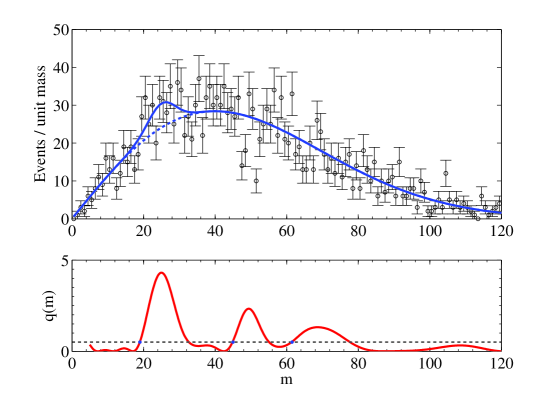
We shall now illustrate the procedure described above with a simple example. Our toy model consists of a gaussian signal (‘mass bump’) on top of a continuous background that follows a Rayleigh distribution, in a mass range [0,120]. The width of the gaussian increases linearly with the mass, representing a case where the mass resolution changes with the mass.

We assume that the background shape is known but its normalization is not, so that it is a free parameter in the fit (i.e. a nuisance parameter), together with the signal location and normalization. We use a binned profile likelihood ratio as our test statistic, where the number of events in each bin is assumed to be Poisson distributed with an expected value

$$E(n_{i})=\mu s_{i}(m)+\beta b_{i}$$ (13)

where $\mu$ is the signal strength parameter, $s_{i}(m)$ corresponds to a gaussian located at a mass $m$, $\beta$ is the background normalization and $b_{i}$ are fixed and given by the Rayleigh distribution. For simplicity of notation we will use in the following $\mathbf{s}=\{s_{i}\}$ and $\mathbf{b}=\{\beta b_{i}\}$. The hypothesis that no signal exists, or equivalently that $\mu=0$, will be referred to as the null hypothesis, $H_{0}$. $\hat{\mu}$ and $\hat{\mathbf{b}}$ will denote maximum likelihood estimators while $\hat{\hat{\mathbf{b}}}$ will denote the conditional maximum likelihood estimator of the background normalization under the null hypothesis.

The test statistic $q(m)$ is defined as:

$$q(m)=-2ln\frac{\mathcal{L}(\mathbf{\hat{\hat{b}}})}{\mathcal{L}(\hat{\mu}\mathbf{s}(m)+\hat{\mathbf{b}})}.$$ (14)

where $\mathcal{L}$ is the likelihood function. An example background-only pseudo-experiment is shown in Fig.1, together with $q(m)$.

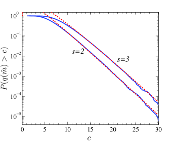
We choose a reference level of $c_{0}=0.5$ and estimate the expected number of upcrossings, as demonstrated in Fig.1, from a set of 100 Monte Carlo simulations of background experiments. This gives $\langle N(c_{0})\rangle=4.34\pm 0.11$, which corresponds to $\mathcal{N}=5.58\pm 0.14$. The distribution of $q(\hat{m})$ is then estimated from a sample of $\sim$1 million background simulations and we compare the tail probabilities to the prediction of (3). The results are shown in Fig.2. The bound of (3) gives an excellent approximation to the observed p-values for large $c$.

Figure 2: (top) Distribution of $q(\hat{m})$. (bottom) Tail probability of $q(\hat{m})$. The solid line shows the result of the Monte Carlo simulation, the dotted red line is the predicted bound (eq. 3) with the estimated $\langle N(c_{0})\rangle$ (see text). The yellow band represents the statistical uncertainty due to the limited sample size.

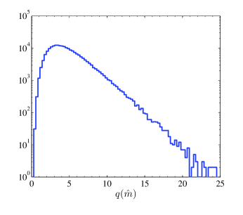
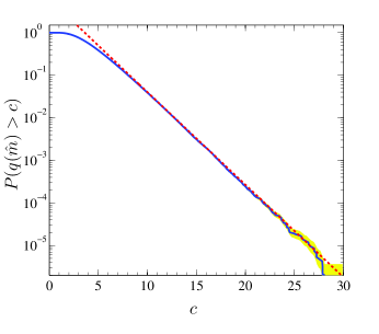
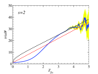
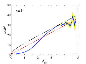
Figure 3 shows the corresponding trial factor, compared to the bound calculated from eq.(3) and the asymptotic approximation of eq.(12).

Figure 3: The trial factor estimated from toy Monte Carlo simulations (solid line), with the upper bound of eq.(3) (dotted black line) and the asymptotic approximation of eq.(12) (dotted red line). The yellow band represents the statistical uncertainty due to the limited sample size.

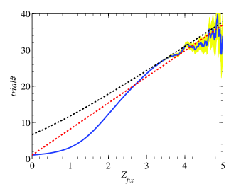
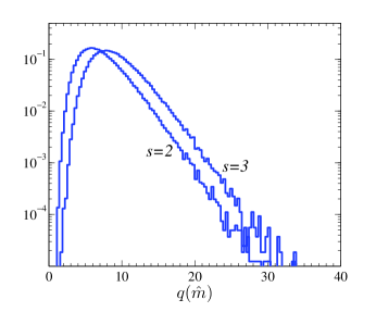
We consider in addition a case where the number of degrees of freedom is more than one. For this purpose, we assume several independent channels, each identical to the one described above, and where the signal normalizations $(\mu_{1},...,\mu_{s})$ are free parameters. (This could represent, for example, a case where one is searching for a resonance in several decay channels, with unknown branching ratios). The reference level is chosen to be $c_{0}=s-1$ as discussed in the previous section. The resulting distributions and trial factors for $s=2,3$ are shown in figures 4 and 5. As before, the the bound (3) agrees with the observed p-value, within statistical variation. The rate at which the asymptotic approximation (11) converges to the bound becomes slower when the number of degrees of freedom increases, making it less accurate, however the trend of linear growth is evident.

Figure 4: (top) Distribution of $q(\hat{m})$ for $s=2,3$. (bottom)Tail probability of $q(\hat{m})$. The solid lines shows the result of the Monte Carlo simulation, the dotted red lines are the predicted bound (eq. 3) with the estimated $\langle N(c_{0})\rangle$ (see text).

Figure 5: The trial factors estimated from toy Monte Carlo simulations (solid line), with the upper bound of eq.(3) (dotted black line) and the asymptotic approximation of eq.(11) (dotted red line). The yellow band represents the statistical uncertainty due to the limited sample size.

4 Conclusions

The look-elsewhere effect presents a case when the standard regularity conditions of Wilks’ theorem do not apply, and so specialized methods are required for estimating tail probabilities in the large sample limit. Such methods however exist, and as we have demonstrated, can provide accurate results under fairly general conditions. The procedure described in this paper consists of estimating the expected number of upcrossings of the likelihood ratio at a low reference level using a small set of Monte Carlo simulations. This can then be related to the expected number of upcrossings at a higher level using Davies’ result (2), providing a bound on the probability of the likelihood ratio exceeding this level, given by (3). The method is easy to implement in practical situations, and the bound converges to the actual tail probability when this probability becomes small. It has further been shown that the trial factor is asymptotically proportional to the effective number of independent search regions and to the fixed-mass significance, allowing for a simple interpretation of the effect as being the result of two factors: the first one is the mere fact that there are more available distinct regions wherein fluctuations can occur, represented by the effective number of independent regions; the second effect is that within each region we further maximize the likelihood by fitting the mass in the neighborhood of the fluctuation, which can be described by adding a degree of freedom to the fit.

5 Acknowledgments

We are indebted to Michael Woodroofe, Luc Demortier and the referee of this paper, for pointing us to the work of Davies davis87 which became the leading thread of this work. We are grateful for the valuable comments made by Luc Demortier in his summary talk in the 2010 Banff workshop banff , and to Michael Woodroofe who spent valuable time in writing to us his impressions on the look elsewhere effect. We also thank Bob Cousins for useful comments and suggestions, BIRS and the organizers of the Banff workshop. One of us (E. G.) is obliged to the Benoziyo center for High Energy Physics, to the Israeli Science Foundation (ISF), the Minerva Gesellschaft, and the German Israeli Foundation (GIF) for supporting this work.

References

- (1) For a general discussion see for example L. Lyons, Open statistical issues in particle physics, The Annals of Applied Statistics 2008, Vol. 2, No. 3, 887-915.
- (2) L. Demortier, P Values and Nuisance Parameters, Proceedings of PHYSTAT-LHC Workshop, 2007, CERN -2008- 001.
- (3) R. B. Davies,Hypothesis testing when a nuisance parameter is present only under the alternative, Biometrika 64 (1977), 247-54.
- (4) R. B. Davies, Hypothesis testing when a nuisance parameter is present only under the alternative, Biometrika 74 (1987), 33-43.
- (5) S.S. Wilks, The large-sample distribution of the likelihood ratio for testing composite hypotheses, Ann. Math. Statist. 9 (1938) 60-62.
- (6) CMS Physics TDR: Volume II, Appendix A.2, J. Phys. G: Nucl. Part. Phys. 34 (2007) 995-1579.
- (7) H. Chernoff, On the distribution of the likelihood ratio, Ann. Math. Statist. 25 (1954) 573-578.
- (8) W. Quayle, Combining chanels with fits, talk given at the PHYSTAT-LHC Workshop, 2007, available at http://phystat-lhc.web.cern.ch/phystat-lhc/program.html.
- (9) Banff International Research Station Workshop on Statistical issues relevant to significance of discovery claims (2010). Workshop site: http://www.birs.ca/events/2010/5-day-workshops/10w5068. Luc Demortier summary talk: http://www.stat.sfu.ca/ lockhart/richard/banff2010/demortier.pdf