Extending the domain of validity of the Lagrangian approximation

Abstract

We investigate convergence of Lagrangian Perturbation Theory (LPT) by analysing the model problem of a spherical homogeneous top-hat in an Einstein-deSitter background cosmology. We derive the formal structure of the LPT series expansion, working to arbitrary order in the initial perturbation amplitude. The factors that regulate LPT convergence are identified by studying the exact, analytic solution expanded according to this formal structure. The key methodology is to complexify the exact solution, demonstrate that it is analytic and apply well-known convergence criteria for power series expansions of analytic functions. The “radius of convergence” and the “time of validity” for the LPT expansion are of great practical interest. The former describes the range of initial perturbation amplitudes which converge over some fixed, future time interval. The latter describes the extent in time for convergence of a given initial amplitude. We determine the radius of convergence and time of validity for a full sampling of initial density and velocity perturbations.

This analysis fully explains the previously reported observation that LPT fails to predict the evolution of an underdense, open region beyond a certain time. It also implies the existence of other examples, including overdense, closed regions, for which LPT predictions should also fail. We show that this is indeed the case by numerically computing the LPT expansion in these problematic cases.

The formal limitations to the validity of LPT expansion are considerably more complicated than simply the first occurrence of orbit crossings as is often assumed. Evolution to a future time generically requires re-expanding the solution in overlapping domains that ultimately link the initial and final times, each domain subject to its own time of validity criterion. We demonstrate that it is possible to handle all the problematic cases by taking multiple steps (LPT re-expansion).

A relatively small number ($\sim 10$) of re-expansion steps suffices to satisfy the time of validity constraints for calculating the evolution of a non-collapsed, recombination-era perturbation up to the current epoch. If it were possible to work to infinite Lagrangian order then the result would be exact. Instead, a finite expansion has finite errors. We characterise how the leading order numerical error for a solution generated by LPT re-expansion varies with the choice of Lagrangian order and of time step size. Convergence occurs when the Lagrangian order increases and/or the time step size decreases in a simple, well-defined manner. We develop a recipe for time step control for LPT re-expansion based on these results.

1 Introduction

Understanding the non-linear growth of structure in an expanding universe has been an active area of research for nearly four decades. Simulations have been instrumental in illustrating exactly what happens to an initial power spectrum of small fluctuations but analytic methods remain essential for elucidating the physical basis of the numerical results. Perturbation theory, in particular, is an invaluable tool for achieving a sophisticated understanding.

The Eulerian and Lagrangian frameworks are the two principal modes of description of a fluid. The fundamental dependent variables in the Eulerian treatment are the density $\rho({\bf x},t)$ and velocity ${\bf v}({\bf x},t)$ expressed as functions of the grid coordinates ${\bf x}$ and time $t$, the independent variables. In perturbation theory the dependent functions are expanded in powers of a small parameter. For cosmology that parameter typically encodes a characteristic small spatial variation of density and/or velocity with respect to a homogeneous cosmology at the initial time. As a practical matter, the first-order perturbation theory becomes inaccurate when the perturbation grows to order unity. Subsequently one must work to higher order to handle the development of non-linearity (see Bernardeau et al. 2002 for a review) or adopt an alternative method of expansion.

In the Lagrangian framework, the fundamental dependent variable is the physical position of a fluid element or particle (terms used interchangeably here). The independent variables are a set of labels ${\bf X}$, each of which follows a fluid element, and the time. Usually ${\bf X}$ is taken as the position of the element at some initial time but other choices are possible. In any case, the physical position and velocity of a fluid element are ${\bf r}={\bf r}({\bf X},t)$ and ${\dot{\bf r}}({\bf X},t)$, respectively. Knowledge of the motion of each fluid element permits the full reconstruction of the Eulerian density and velocity fields. In cosmological applications of Lagrangian perturbation theory (LPT), just like Eulerian perturbation theory, the dependent variables are expanded in terms of initial deviations with respect to a homogeneous background. The crucial difference is that the basis for the expansion is the variation in the initial position and position-derivative not the variation in the initial fluid density and velocity. The Eulerian density and velocity may be reconstructed from knowledge of the Lagrangian position using exact non-perturbative definitions. A linear approximation to the displacement field results in a non-linear expression for the density contrast. The Lagrangian description is well-suited to smooth, well-ordered initial conditions; a single fluid treatment breaks down once particle crossings begin, caustics form and the density formally diverges.

First-order LPT was originally introduced by Zel’Dovich (1970) to study the formation of non-linear structure in cosmology. In his treatment the initial density field was taken to be linearly proportional to the initial displacement field (the “Zeldovich approximation”). These results were extended by many authors (Moutarde et al. 1991; Buchert 1992; Bouchet et al. 1992; Buchert & Ehlers 1993; Buchert 1994; Munshi et al. 1994; Catelan 1995; Buchert 1995; Bouchet et al. 1995; Bouchet 1996; Ehlers & Buchert 1997). The work pioneered by Bouchet focused on Zeldovich initial conditions and established the link between LPT variables and statistical observables. The work by Buchert as well as the paper by Ehlers & Buchert (1997) formalised the structure of the Newtonian perturbative series for arbitrary initial conditions. A general relativistic version of the Zeldovich approximation was developed by Kasai (1995) and other relativistic descriptions of the fluid in its rest frame were investigated by Matarrese & Terranova (1996) and Matarrese, Pantano & Saez (1993, 1994). LPT has been used for many applications including, recently, the construction of non-linear halo mass functions by Monaco (1997) and Scoccimarro & Sheth (2002).

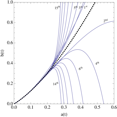
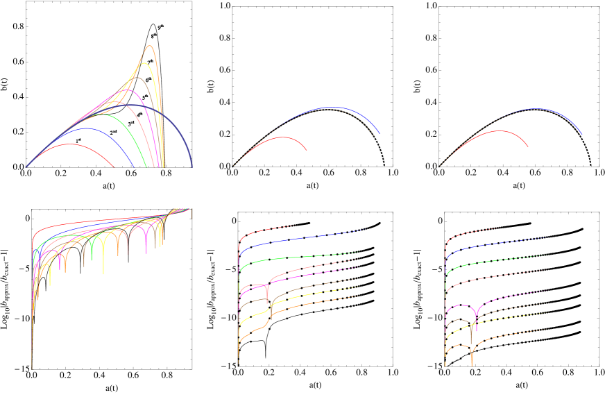
Not much has been written about the convergence of LPT although LPT expansions are routinely employed. Sahni & Shandarin (1996) pointed out that the formal series solution for the simplest problem, the spherical top-hat, did not converge for the evolution of homogeneous voids. Figure 1 illustrates the conundrum that the LPT approximations diverge from the exact solution in a manner that worsens as the order of the approximation increases. The details will be described in the next section.

This paper explores LPT convergence for the spherical top-hat and identifies the root cause for the lack of convergence. The analysis naturally suggests a means of extending the range of validity of LPT. This generalisation of LPT guarantees convergence to the exact solution of the model problem at all times prior to the occurrence of the first caustic.

Tatekawa (2007) attempted to treat the divergence by applying the Shanks transformation to the LPT series. Although non-linear transformations can sum a divergent series, the correct answer is not guaranteed; comparison of several different methods is usually necessary to yield trustworthy results. Other approaches include the Shifted-Time-Approximation (STA) and Frozen-Time-Approximation (FTA) which have been investigated by Karakatsanis, Buchert & Melott (1997). These schemes modify lower order terms to mimic the behavior of higher order terms and/or extend the range of applicability in time. None of these techniques are considered here.

Figure 1: The time-dependent scale factor $b$ of an initial spherical top-hat perturbation is plotted as a function of the background scale factor $a$. The perturbation is a pure growing mode, i.e. the density and velocity perturbations vanish at $t=0$. The black dotted line is the exact solution. The smooth blue lines are the LPT results obtained by working successively to higher and higher order. Series with even (odd) final order lie below (above) the exact solution. Roughly speaking, LPT converges only for $a\mathbin{\lower 3.0pt\hbox{$\hbox to0.0pt{\raise 5.0pt\hbox{$\char 60\relax$}\hss}\mathchar 29208\relax$}}0.2$. Beyond that point the higher order approximations deviate from the exact solution more than lower order ones.

The organisation follows: §2 sketches the model problem, the evolution of a uniform sphere in a background homogeneous Einstein-deSitter cosmology. The LPT equations, the structure of the formal series and the term-by-term solution are outlined. §3 discusses the complexification of the LPT solution and convergence of the series. This section introduces the “radius of convergence” and the “time of validity” for LPT. §4 outlines the real and complex forms of the parametric solution and sets forth the equations that must be solved to locate the poles which govern the convergence. §5 presents numerical results for the time of validity and radius of convergence for a full range of possible initial conditions for the top-hat. The notion of mirror model symmetry is introduced and used to explain a connection in the convergence for open and closed models. §6 shows that the time of validity may be extended by re-expanding the solution in overlapping domains that ultimately link the initial and final times, each domain subject to an individual time of validity criterion. The feasibility of this method is demonstrated in some examples. §7 summarises the work.

2 The model problem and formal series solution

This section describes the governing equations, the initial physical conditions, the formal structure of the LPT series solution and the order-by-order solution.

2.1 Newtonian treatment

Consider evolution on sub-horizon scales after recombination in a matter-dominated universe. A Newtonian treatment of gravity based on solving Poisson’s equation for the scalar potential and on evaluating the force in terms of the gradient of the potential gives an excellent approximation for non-relativistic dynamics. When there are no significant additional forces on the fluid element (e.g. pressure forces) then it is straightforward to eliminate the gradient of the potential in favour of ${\ddot{\bf r}}$, the acceleration. The governing equations are

$$\nabla_{x}\cdot{\ddot{\bf r}} = -4\pi G\rho({\bf x},t)$$ (1)

$$\nabla_{x}\times{\ddot{\bf r}} = 0$$ (2)

where $\rho({\bf x},t)$ is the background plus perturbation density, $G$ is Newton’s gravitational constant and $\nabla_{x}$ is the Eulerian gradient operator. In the Lagrangian treatment, the independent variables are transformed $({\bf x},t)\to({\bf X},t)$ and the particle position ${\bf r}={\bf r}({\bf X},t)$ adopted as the fundamental dependent quantity. For clarity note that ${\bf x}$ refers to a fixed Eulerian grid not a comoving coordinate.

2.2 Spherical top-hat

The starting physical configuration is a compensated spherical perturbation in a homogeneous background cosmology. The perturbation encompasses a constant density sphere about the centre of symmetry and a compensating spherical shell. The shell that surrounds the sphere may include vacuum regions plus regions of varying density. Unperturbed background extends beyond the outer edge of the shell. Physical distances are measured with respect to the centre of symmetry. At initial time $t_{0}$ the background and the innermost perturbed spherical region (hereafter, “the sphere”) have Hubble constants $H_{0}$ and $H_{p0}$, and densities $\rho_{0}$ and $\rho_{p0}$, respectively. Let $r_{b,0}$ ($r_{p,0}$) be the physical distance from the centre of symmetry to the inner edge of the background (to the outer edge of the sphere) at the initial time. Let $a_{0}$, $b_{0}$ be the initial scale factors for the background and the sphere respectively. Two sets of Lagrangian coordinates $Y=r_{b,0}/a_{0}$ and $X=r_{p,0}/b_{0}$ are defined. A gauge choice sets $a_{0}=b_{0}$. Appendix A provides a figure and gives a somewhat more detailed chain of reasoning that clarifies the construction of the physical and Lagrangian coordinate systems. The initial perturbation is characterised by the independent parameters

$$\delta = \frac{\rho_{p0}}{\rho_{0}}-1$$

$$\delta_{v} = \frac{H_{p0}}{H_{0}}-1.$$ (3)

Finally, assume that the background cosmology is critical $\Omega_{0}=1$. The perturbed sphere has

$$\Omega_{p0}=\frac{1+\delta}{(1+\delta_{v})^{2}}.$$ (4)

The physical problem of interest here is the future evolution of an arbitrary initial state unconstrained by the past history. In general, the background and the perturbation can have different big bang times. Initial conditions with equal big bang times will be analysed as a special case of interest and imply an additional relationship between $\delta$ and $\delta_{v}$.

While the previous paragraphs summarise the set up, they eschew the complications in modelling an inhomogeneous system in terms of separate inner and outer homogeneous universes. For example, matter motions within the perturbed inner region may overtake the outer homogeneous region so that there are problem-specific limits on how long solutions for the scale factors $a(t)$ and $b(t)$ remain valid. The appendix shows that there exist inhomogeneous initial configurations for which the limitations arising from the convergence of the LPT series are completely independent of the limitations associated with collisions or crossings of inner and outer matter-filled regions. A basic premise of this paper is that it is useful to explore the limitations of the LPT series independent of the additional complications that inhomogeneity entails.

2.3 Equation governing scale factors

During the time that the spherical perturbation evolves as an independent homogeneous universe it may be fully described in terms of the motion of its outer edge $r_{p}$. Write

$$r_{p}(t)=b(t)X$$ (5)

where $b(t)$ is the scale factor and $X$ is the Lagrangian coordinate of the edge. The initial matter density of the homogeneous sphere $\rho(X,t_{0})=\rho_{p0}=\rho_{0}(1+\delta)$. The physical density of the perturbation at time $t$ is

$$\rho(X,t)=\frac{\rho(X,t_{0})J(X,t_{0})}{J(X,t)}$$ (6)

where the Jacobian of the transformation relating the Lagrangian and physical spaces is

$$J(X,t)=\det\left(\frac{\partial{\vec{r}}}{\partial{\vec{X}}}\right).$$ (7)

Since eq. (5) implies $J(X,t)=b(t)^{3}$ and the choice $a_{0}=b_{0}$ implies $J(X,t_{0})=a_{0}^{3}$ the perturbation matter density at later times is

$$\rho_{p}(t)=\frac{\rho_{0}(1+\delta)a_{0}^{3}}{b(t)^{3}}.$$ (8)

Substituting for $\rho_{p}$ and $r_{p}$ in eq. (1) gives

$$\frac{{\ddot{b}}}{b}=-\frac{1}{2}\frac{H_{0}^{2}a_{0}^{3}(1+\delta)}{b^{3}}$$ (9)

with initial conditions $b(t_{0})=a_{0}$ and ${\dot{b}}(t_{0})={\dot{a}}_{0}(1+\delta_{v})$. The curl of the acceleration (i.e. eq. (2)) vanishes by spherical symmetry. The corresponding equation for the background scale factor is

$$\frac{{\ddot{a}}}{a}=-\frac{1}{2}\frac{H_{0}^{2}a_{0}^{3}}{a^{3}}$$ (10)

with initial conditions $a(t_{0})=a_{0}$ and ${\dot{a}}(t_{0})={\dot{a}}_{0}=a_{0}H_{0}$. The solution for $b(t)$ will be expressed in terms of its deviations from $a(t)$.

In summary, the physical setup is an $\Omega_{0}=1$ background model and a compensated spherical top-hat (over- or underdense). The properties of interest are the relative scale factors $a(t)/a_{0}$ and $b(t)/a_{0}$ (the choice of $a_{0}$ is arbitrary and $b_{0}=a_{0}$). The evolution of the relative scale factors is fully specified by $H_{0}$, $H_{p0}$ and $\Omega_{p0}$ at time $t_{0}$. The perturbed physical quantities, $H_{p0}$ and $\Omega_{p0}$, may be equivalently specified by a choice of $\delta$ and $\delta_{v}$. Appendix A contains a systematic description and enumerates degrees of freedom, parameters, constraints, etc.

2.4 Perturbations in phase space

The initial density and velocity perturbations are taken to be of the same order in the formalism developed by Buchert (1992, 1994), Buchert & Ehlers (1993) and Ehlers & Buchert (1997). We assume the same ordering here. Write the initial perturbation ($\delta$, $\delta_{v}$) in terms of magnitude $\Delta$ and angle $\theta$

$$\Delta=\sqrt{\delta^{2}+\delta_{v}^{2}}$$ (11)

so that

$$\delta = \Delta\cos\theta$$ (12)

$$\delta_{v} = \Delta\sin\theta.$$ (13)

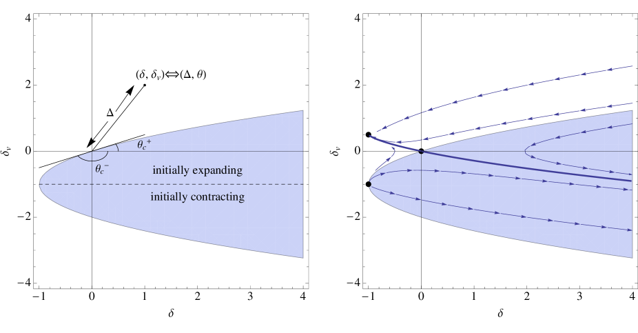
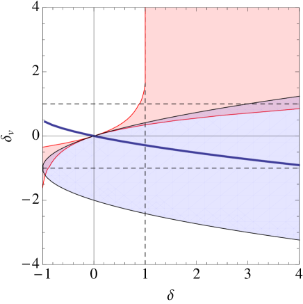
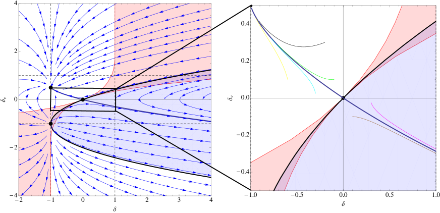
To map physical perturbations $(\delta,\delta_{v})$ in a unique manner to $(\Delta,\theta)$ adopt the ranges $\Delta\geq 0$ and $-\pi<\theta\leq\pi$. Figure 2 (left panel) shows the phase space of initial perturbations. Since density is non-negative the regime of physical interest is $\delta\geq-1$. Open (closed) models with positive (negative) total energy are the regions that are unshaded (shaded). Initially expanding models, $1+\delta_{v}>0$, lie above the horizontal dashed line. The right panel of figure 2 summarises the overall evolution of the system. The initial choice of $\delta$ and $\delta_{v}$ dictates the trajectory in the plane. Cosmologically relevant initial conditions generally assume there to be no perturbation at $t=0$. We adopt the name “Zeldovich” initial conditions for models that satisfy this condition. This establishes a specific relation between $\delta$ and $\delta_{v}$ which is indicated by the sold blue line. The exact mathematical relationship is given in §5.4. Starting from a general initial point ($\delta,\delta_{v}$), the system as it evolves traces out a curve in phase space indicated by the blue arrows. There are three fixed points visible. The origin $(\delta,\delta_{v})\equiv(0,0)$, which corresponds to a unperturbed background model, is a saddle point. The vacuum static model at point $(-1,-1)$ is a unstable node and the vacuum, expanding model at $(-1,0.5)$ is a degenerate attracting node. Far to the right and below the dashed line the models collapse to a future singularity. The phase portrait illustrates that the trajectories either converge to the vacuum, expanding model or to the singular, collapsing model. The equations that govern the flow and further relevance of the Zeldovich solution is discussed in §6.2 and §5.4.

Figure 2: Phase diagram of density and velocity perturbations $(\delta,\delta_{v})$. Physical initial conditions require $-1<\delta<\infty$ and $-\infty<\delta_{v}<\infty$. The left panel highlights the qualitatively different initial conditions. The shaded (unshaded) region corresponds to closed (open) model with negative (positive) total energy. For small $\Delta$, models with $\theta_{c}^{-}<\theta<\theta_{c}^{+}$ are closed. Initially expanding and contracting models are separated by the dashed horizontal line ($\delta_{v}=-1$). The right panel shows the evolution of $\delta$ and $\delta_{v}$. The solid blue line corresponds to the “Zeldovich” condition i.e no perturbation at $t=0$. The points $(-1,-1),(-1,0.5)$ and $(0,0)$ are unstable, stable and saddle fixed points of the phase space flow. The flow lines (indicated by the blue vectors) converge along the Zeldovich curve either to the stable fixed point at $(-1,0.5)$ or move parallel to the Zeldovich curve to a future density singularity. Further discussion follows in §5.4 and §6.2.

2.5 Generating the Lagrangian series solution

The scale factor is formally expanded

$$b(t)=\sum_{n=0}^{\infty}b^{(n)}(t)\Delta^{n}$$ (14)

where $b^{(n)}$ denotes an $n$-th order term. The initial conditions are

$$b(t_{0}) = a(t_{0})$$ (15)

$${\dot{b}}(t_{0}) = \dot{a}_{0}(1+\delta_{v})=\dot{a}_{0}(1+\Delta\sin\theta).$$ (16)

Substitute the expansion for $b(t)$ into eq. (9), equate orders of $\Delta$ to give at zeroth order

$${\ddot{b}}^{(0)}+\frac{1}{2}\frac{H_{0}^{2}a_{0}^{3}}{{b^{(0)}}^{2}}=0$$ (17)

which is identical in form to eq. (10) for the unperturbed background scale factor. The initial conditions at zeroth order:

$$b^{(0)}(t_{0}) = a_{0}$$ (18)

$${\dot{b}}^{(0)}(t_{0}) = {\dot{a}}_{0}.$$ (19)

The equation and initial conditions for $b^{(0)}(t)$ simply reproduce the background scale factor evolution $b^{(0)}(t)=a(t)$. Without loss of generality assume that the background model has big bang time $t=0$ so that

$$a(t)=a_{0}\left(\frac{t}{t_{0}}\right)^{2/3}=a_{0}\left(\frac{3H_{0}t}{2}\right)^{2/3}.$$ (20)

At first order

$${\ddot{b}}^{(1)}-\frac{H_{0}^{2}a_{0}^{3}b^{(1)}}{a^{3}}=-\frac{1}{2}\frac{H_{0}^{2}a_{0}^{3}\cos\theta}{a^{2}}$$ (21)

and, in general,

$${\ddot{b}}^{(n)}-\frac{H_{0}^{2}a_{0}^{3}b^{(n)}}{a^{3}}=S^{(n)}$$ (22)

where $S^{(n)}$ depends upon lower order approximations ($b^{(0)},b^{(1)}\dots b^{(n-1)}$) as well as $\theta$. The first few are:

$$S^{(2)} = -\frac{1}{2}\frac{H_{0}^{2}a_{0}^{3}}{a^{4}}\left[b^{(1)}\left\{3b^{(1)}-2a\cos\theta\right\}\right]$$ (23)

$$S^{(3)} = -\frac{1}{2}\frac{H_{0}^{2}a_{0}^{3}}{a^{5}}\left[b^{(1)}\left\{-4\left(b^{(1)}\right)^{2}+6ab^{(2)}+3ab^{(1)}\cos\theta\right\}-2a^{2}b^{(2)}\cos\theta\right]$$ (24)

$$S^{(4)} = -\frac{1}{2}\frac{H_{0}^{2}a_{0}^{3}}{a^{6}}\left[\left(b^{(1)}\right)^{2}\left\{5\left(b^{(1)}\right)^{2}-12ab^{(2)}-4ab^{(1)}\cos\theta\right\}+\right.$$ (25)

$$\phantom{-\frac{1}{2}\frac{H_{0}^{2}a_{0}^{3}}{a^{6}}\left[\right.}\left.6a^{2}b^{(1)}\left\{b^{(3)}+b^{(2)}\cos\theta\right\}+3a^{2}\left(b^{(2)}\right)^{2}-2a^{3}b^{(3)}\cos\theta\right].$$

These terms can be easily generated by symbolic manipulation software. The initial conditions are

$$b^{(1)}(t_{0}) = 0$$ (26)

$${\dot{b}}^{(1)}(t_{0}) = {\dot{a}}_{0}\sin\theta$$ (27)

and for $n>1$

$$b^{(n)}(t_{0}) = 0$$ (28)

$${\dot{b}}^{(n)}(t_{0}) = 0.$$ (29)

The ordinary differential equations for $b^{(n)}$ may be solved order-by-order.

To summarise, the structure of the hierarchy and the simplicity of the initial conditions allows the evaluation of the solution at any given order in terms of the solutions with lower order. This yields a formal expansion for the scale factor of the sphere

$$b=\sum_{n=0}^{\infty}b^{(n)}(t)\Delta^{n}$$ (30)

which encapsulates the Lagrangian perturbation treatment. The right hand size explicitly depends upon the size of the perturbation and time and implicitly upon $a_{0}$, $H_{0}$, and $\theta$. This hierarchy of equations is identical to that generated by the full formalism developed by Buchert and collaborators when it is applied to the top-hat problem. The convergence properties in time and in $\Delta$ are distinct; a simple illustrative example of this phenomenon is presented in Appendix B.

3 Convergence properties of the LPT series solution

The series solution outlined in the previous section does not converge at all times. Figure 1 is a practical demonstration of this non-convergence for the case of an expanding void. An understanding of the convergence of the LPT series is achieved by extending the domain of the expansion variable $\Delta$ from the real positive axis to the complex plane.

3.1 Complexification

The differential eq. (9) and initial conditions for the physical system are

$$\ddot{b}(t) = -\frac{1}{2}\frac{H_{0}^{2}a_{0}^{3}(1+\Delta\cos\theta)}{b(t)^{2}}$$

$$b(t_{0}) = a_{0}$$

$$\dot{b}(t_{0}) = {\dot{a}}_{0}(1+\Delta\sin\theta)$$ (31)

where $t$, $b(t)$, $\Delta$ and all zero-subscripted quantities are real. This set may be extended by allowing $\Delta$ and $b$ to become complex quantities, denoted hereafter, $\bm{\Delta}$ and ${\bf b}$, while the rest of the variables remain real. The complex set is

$$\ddot{\bf b}(t) = -\frac{1}{2}\frac{H_{0}^{2}a_{0}^{3}(1+\bm{\Delta}\cos\theta)}{{\bf b}(t)^{2}}$$

$${\bf b}(t_{0}) = a_{0}$$

$$\dot{\bf b}(t_{0}) = {\dot{a}}_{0}(1+\bm{\Delta}\sin\theta).$$ (32)

The theory of differential equations (for example, Chicone 2006) guarantees that the solution to a real initial value problem is unique and smooth in the initial conditions and parameters of the equation and can be extended in time as long as there are no singularities in the differential equation (hereafter, the maximum extension of the solution). First, note that each complex quantity in eq. (3.1) may be represented by a real pair, i.e. ${\bf b}=u+iv$ by pair $\{u,v\}=\{\Re{\bf b},\Im{\bf b}\}$ and ${\bf\Delta}=x+iy$ by pair $\{x,y\}=\{\Re{\bf\Delta},\Im{\bf\Delta}\}$. The basic theory implies continuity and smoothness of solution $u$ and $v$ with respect to initial conditions and parameters $x$ and $y$. Second, observe that the Cauchy-Riemann conditions $u_{x}=v_{y}$ and $u_{y}=-v_{x}$ are preserved by the form of the ordinary differential equation. Since the initial conditions and parameter dependence are holomorphic functions of $\bm{\Delta}$ it follows that ${\bf b}(t,\bm{\Delta})$ is a holomorphic function of $\bm{\Delta}$ at times $t$ within the maximum extension of the solution.

Inspection shows that the differential equation is singular only at ${\bf b}=0$. For a particular value of $\bm{\Delta}=\bm{\Delta}^{\prime}$, the solution to the initial value problem can be extended to a maximum time $t_{mx}$ such that ${\bf b}(\bm{\Delta}^{\prime},t_{mx})=0$ or to infinity. The existence of a finite $t_{mx}$ signals that a pole in the complex analytic function ${\bf b}(\bm{\Delta},t)$ forms at $\bm{\Delta}=\bm{\Delta}^{\prime}$ and $t=t_{mx}$. For times $t$ such that $t_{0}\leq t<t_{mx}$, the solution $b(\bm{\Delta},t)$ is analytic in a small neighbourhood around the point $\bm{\Delta}^{\prime}$. Of course, there may be poles elsewhere in the complex $\bm{\Delta}$ plane.

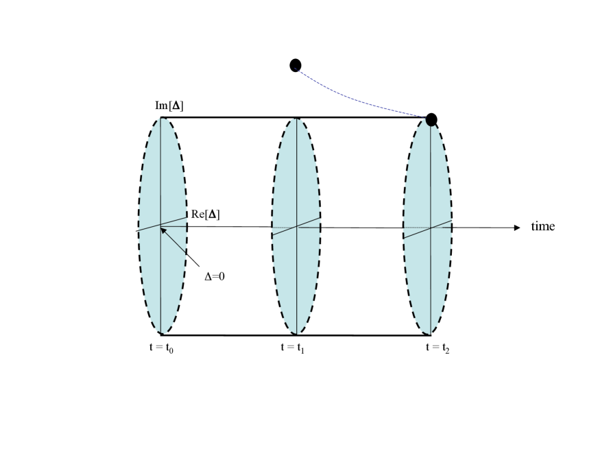
The relationship between the original, real-valued physical problem and the complexified system is the following. In the original problem $\Delta$ is a real, positive quantity at $t_{0}$. LPT is a power series expansion in $\Delta$ about the origin (the point $\Delta=0$). LPT’s convergence at any time $t$ can be understood by study of the complexified system. Consider the complex disk ${\cal D}$ centred on the origin and defined by $|\bm{\Delta}|<\Delta$. At $t_{0}$ each point in ${\cal D}$ determines a trajectory ${\bf b}(\bm{\Delta},t)$ for the complexified system extending to infinity or limited to finite time $t=t_{mx}(\bm{\Delta})$ because of the occurrence of a pole. The time of validity is defined as $T(\Delta)=\min_{\cal D}t_{mx}$, i.e. the minimum $t_{mx}$ over the disk. Since there are no poles in ${\cal D}$ at $t_{0}$ the time of validity is the span of time when ${\cal D}$ remains clear of any singularities. If a function of a complex variable is analytic throughout an open disk centred around a given point in the complex plane then the series expansion of the function around that point is convergent (Brown & Churchill 1996). The LPT expansion for the original problem converges for times less than the time of validity because the complex extension ${\bf b}(\bm{\Delta},t)$ is analytic throughout ${\cal D}$ for $t<T(\Delta)$. If $\Delta_{1}<\Delta_{2}$ then, in an obvious notation, the disks are nested ${\cal D}(\Delta_{1})\subset{\cal D}(\Delta_{2})$ and the times of validity are ordered $T(\Delta_{1})\geq T(\Delta_{2})$.

This idea is shown in figure 3. No singularities are present for the initial conditions at $t_{0}$; at $t_{1}$ a singularity is present outside the disk but it does not prevent the convergence of the LPT expansion with $\Delta$ equal to the disk radius shown; at $t_{2}$ a singularity is present in the disk or on its boundary and it may interfere with convergence.

Figure 3: This figure is a schematic illustration of how the time of validity is determined. The initial conditions imply a specific, real $\Delta$ at time $t_{0}$. The LPT series is an expansion about $\Delta=0$, convergent until a pole appears at some later time within the disk of radius $\Delta$ (shown in cyan) in the complex $\bm{\Delta}$ plane. Typically, the pole’s position forms a curve (blue dashed) in the three dimensional space $(\Re[\bm{\Delta}],\Im[\bm{\Delta}],t)$. The black dots mark the pole at times $t_{1}$ and $t_{2}$. At $t_{1}$ the pole does not interfere with the convergence of the LPT series; at $t_{2}$ it does. The time of validity may be determined by a pole that appears within the disk without moving through the boundary (not illustrated).

A distinct but related concept is the maximum amplitude perturbation for which the LPT expansion converges at the initial time and at all intermediate times up to a given time. The radius of convergence $R_{\Delta}(t)$ is the maximum disk radius $\Delta$ for which $t>T(\Delta)$. Because the disks are nested if $t_{1}<t_{2}$ then $R_{\Delta}(t_{1})\geq R_{\Delta}(t_{2})$.

The time of validity and the radius of convergence are inverse functions of each other. If the initial perturbation is specified, i.e. $\Delta$ is fixed, and the question to be answered is “how far into the future does LPT work?” then the time of validity gives the answer. However, if the question is “how big an initial perturbation will be properly approximated by LPT over a given time interval?” then the radius of convergence provides the answer.

Finally, note that one can trivially extend this formalism to deal with time intervals in the past.

3.2 Calculating radius of convergence and time of validity

The following recipe shows how to calculate the radius of convergence $R_{\Delta}(t)$ and the time of validity $T(\Delta)$ efficiently. Fix $a_{0}$, $H_{0}$, $t_{0}$ and $\theta$; these are all real constants set by the initial conditions. Assume that it is possible to find ${\bf b}(\bm{\Delta},t)$ for complex $\bm{\Delta}$ and real $t$ by solving eq. (3.1). There exist explicit expressions for ${\bf b}$ as will be shown later.

Start with $t=t_{0}$ and $R_{\Delta}(t)=\infty$. The iteration below maps out $R_{\Delta}(t)$ by making small increments in time $\delta t$.

• Store old time $t_{previous}=t$, choose increment $\delta t$ and form new time of interest $t=t_{previous}+\delta t$.

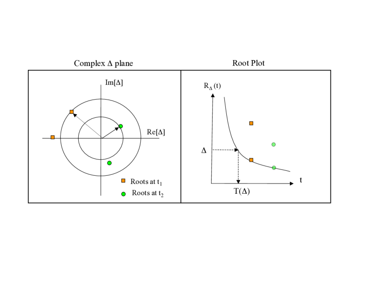
• Locate all the $\bm{\Delta}$ which solve ${\bf b}(\bm{\Delta},t)=0$. The roots correspond to poles in the complex function. Find the root closest to the origin and denote its distance as $|\bm{\Delta}_{near}|$.

• The radius of convergence is $R_{\Delta}(t)=\min(|\bm{\Delta}_{near}|,R_{\Delta}(t_{previous}))$.

• Continue.

Since $R_{\Delta}$ is decreasing, the inversion to form $T(\Delta)$ is straightforward. Figure 4 shows a schematic cartoon of the construction process.

Figure 4: A schematic illustration of the radius of convergence and the time of validity. The left panel shows the location of poles in the complex $\bm{\Delta}$ plane at times $t_{1}$ and $t_{2}$, denoted by orange squares and green dots, respectively. At a fixed time, the pole nearest the origin determines the disk (black circle) within which a series expansion about the origin converges. The right panel shows $|\bm{\Delta}|$ for $t_{1}$ and $t_{2}$. The black line is $R_{\Delta}(t)$, the minimum $|\bm{\Delta}|$ calculated for a continuous range of times (where $t_{0}$, the initial time, lies far to the left). The arrows show how the time of validity is inferred for a given $\Delta$.

4 Explicit solutions

The usual parametric representation provides an efficient method to construct an explicit complex representation for ${\bf b}(\bm{\Delta},t)$.

4.1 Real (physical) solutions

The original system eq. (3.1) depends upon $a_{0}$, $H_{0}$, $\theta$ and $\Delta$. The assumed Einstein-deSitter background has $a_{0}>0$ and ${\dot{a}}_{0}>0$; as defined, the perturbation amplitude $\Delta\geq 0$ and the relative density and velocity components are determined by phase angle $\theta$ with $-\pi<\theta\leq\pi$. The quantity $(1+\Delta\cos\theta)$ is proportional to total density and must be non-negative. The sign of ${\dot{b}}_{0}$ is the sign of $1+\Delta\sin\theta$ and encodes expanding and contracting initial conditions.

Briefly reviewing the usual physical solution, the integrated form is

$${\dot{b}}^{2}=H_{0}^{2}a_{0}^{3}\left[\frac{(1+\Delta\cos\theta)}{b}+\frac{(1+\Delta\sin\theta)^{2}-(1+\Delta\cos\theta)}{a_{0}}\right].$$ (33)

The combination

$$E(\Delta,\theta)=(1+\Delta\sin\theta)^{2}-(1+\Delta\cos\theta)$$ (34)

is proportional to the total energy of the system. If $E>0$ the model is open and if $E<0$ it is closed and will re-collapse eventually. Figure 2 shows the parabola $E=0$ which separates open and closed regions. For infinitesimal $\Delta$ the line of division has slope $\tan\theta=1/2$. Models with $\theta\in[\theta_{c}^{-},\theta_{c}^{+}]=[-\pi+\tan^{-1}(1/2),\tan^{-1}(1/2)]=[-2.68,0.46]$ are closed while those outside this range are open.

There are four types of initial conditions (positive and negative $E$, positive and negative ${\dot{b}}_{0}$) and four types of solutions, shown schematically in figure 5. The solutions have well-known parametric forms involving trigonometric functions of angle $\eta$ or $i\eta$ (see Appendix C). The convention adopted here is that the singularity nearest the initial time $t_{0}$ coincides with $\eta=0$ and is denoted $t_{bang}^{+}$ ($t_{bang}^{-}$) for initially expanding (contracting) solutions (see figure 5). The time interval between the singularity and $t_{0}$ is $t_{age}=|t_{0}-t_{bang}^{\pm}|\geq 0$.

Figure 5: Scale factor as a function of time. The initial conditions ($b_{0}=a_{0}=1$ and varying ${\dot{b}}_{0}$) are given at time $t_{0}$ (dashed blue line). The left (right) panel illustrates initially expanding (contracting) models. $t_{bang}^{\pm}$ corresponds to $\eta=0$; $t_{coll}$ to $\eta=2\pi$. For expanding solutions $t_{age}=t_{0}-t_{bang}^{+}$ is the time interval since the initial singularity and $t_{coll}$ is the future singularity for closed models. For contracting solutions $t_{age}=t_{bang}^{-}-t_{0}$ is the time until the final singularity and $t_{coll}$ is the past singularity for closed models.

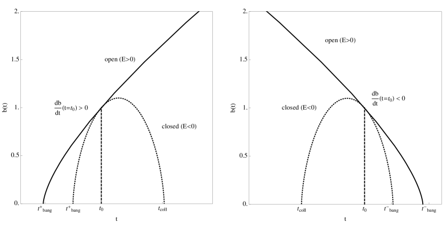
The parametric solution for the models can be written as

$$b(\eta,\Delta,\theta) = \frac{a_{0}}{2}\frac{(1+\Delta\cos\theta)}{\left[-E(\Delta,\theta)\right]}(1-\cos\eta)$$

$$t(\eta,\Delta,\theta) = t_{0}\pm\left(\frac{1}{2H_{0}}\frac{(1+\Delta\cos\theta)}{\left[-E(\Delta,\theta)\right]^{3/2}}(\eta-\sin\eta)-t_{age}(\Delta,\theta)\right).$$ (35)

The plus and minus signs give the solution for initially expanding and initially contracting models respectively. Parameter $\eta$ is purely real for closed solutions and purely imaginary for open solutions. The distance to the nearest singularity is

$$t_{age}=\int_{b=0}^{b=a_{0}}\frac{db}{[{\dot{b}}^{2}]^{1/2}}=\frac{1}{H_{0}}\int_{y=0}^{y=1}\frac{dy}{\left[(1+\Delta\cos\theta)y^{-1}+E(\Delta,\theta)\right]^{1/2}}.$$ (36)

The second equality uses eq. (33) and the substitution $y=b/a_{0}$.

4.2 Complex extension

To extend the above parametric solution to the complex plane, one might guess the substitution $\Delta\rightarrow\Delta e^{i\phi}$ where $-\pi<\phi\leq\pi$ in eq. (35) and eq. (36). The physical limit is $\phi=0$. However, this leads to two problems. First, the integral for $t_{age}$ can have multiple extensions that agree for physical $\phi=0$ but differ elsewhere including the negative real axis. This is tied to the fact that the operations of integration and substitution $\Delta\rightarrow\Delta e^{i\phi}$ do not commute because of the presence of the square root in the expression for $t_{age}$. A second related problem is the presence of multiple square roots in the parametric form for $t$. These give rise to discontinuities along branch cuts such that one parametric form need not be valid for the entire range of $\phi$, but instead the solution may switch between different forms. Directly extending the parametric solution is cumbersome.

However, the original differential eq. (3.1) is manifestly single-valued. The equation can be integrated forward or backward numerically to obtain the correct solution for complex $\bm{\Delta}$. One can then match the numerical solution to the above parametric forms to select the correct branch cuts. This procedure was implemented to obtain the form for all $\bm{\Delta}$ and $\theta$. The main result is that the solution space for all $\theta$ and $\bm{\Delta}$ is completely spanned by complex extensions of the two real parametric forms which describe initially expanding and contracting solutions. The expressions for ${\bf t}_{age}$ and details are given in Appendix C.3.

The traditional textbook treatment relating physical cosmological models with real $\Omega>1$ and $\Omega<1$ typically invokes a discrete transformation $\eta\rightarrow i\eta$ in the parametric forms and one verifies that this exchanges closed and open solutions. However, starting from the second order differential equation it is straightforward to use the same type of reasoning as above to construct an explicit analytic continuation from one physical regime to the other.

In addition, note that the differential equation and its solution remain unchanged under the simultaneous transformations $\bm{\Delta}\rightarrow-\bm{\Delta}$ and $\theta\rightarrow\theta+\pi$. Every complex solution with $-\pi<\theta\leq 0$ can be mapped to a complex solution with $0<\theta\leq\pi$ and vice-versa. For determining the radius of convergence and the time of validity the whole disk of radius $|\bm{\Delta}|$ is searched for poles so it suffices to consider a restricted range of $\theta$ to handle all physical initial conditions.

4.3 Poles

The condition ${\bf b}=0$ signals the presence of a pole. Inspection of the parametric form shows that this condition can occur only when $\eta=0$ or $\eta=2\pi$. The corresponding time

$${\bf t}(\bm{\Delta},\theta) = \left\{\begin{array}[]{cc}t_{0}\pm\left(\frac{\pi}{H_{0}}\frac{(1+\bm{\Delta}\cos\theta)}{\left[-{\bf E}(\bm{\Delta})\right]^{3/2}}-{\bf t_{age}}(\bm{\Delta})\right)&(\eta=2\pi)\\ t_{0}\mp{\bf t_{age}}(\bm{\Delta})&(\eta=0)\\ \end{array}\right.$$ (39)

is immediately inferred. Since the independent variable $t$ is real the transcendental equation

$$\Im{\bf t}(\bm{\Delta},\theta)=0$$ (40)

must be solved. It is straightforward to scan the complex $\bm{\Delta}$ plane and calculate ${\bf t}$ to locate solutions. Each solution gives a root of ${\bf b}=0$ and also implies the existence of a pole at the corresponding $\bm{\Delta}$. Note that relying upon the parametric solutions is a far more efficient method for finding the poles than integrating the complex differential equations numerically. We have verified that both methods produce the same results.

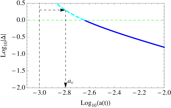
In practice, we fix $\theta$, scan a large area of the complex $\bm{\Delta}$ plane, locate all purely real ${\bf t}$ and save the $\{\bm{\Delta},t\}$ pairs. These are used to create a scatter plot of $|\bm{\Delta}|$ as a function of time (hereafter the “root plot”). Generally, the location of the poles varies smoothly with $t$ and continuous loci of roots are readily apparent. Finding $R_{\Delta}$ and $T(\Delta)$ follows as indicated in figure 4.

5 Results from the complex analysis

Root plots were calculated for a range of angles $0\leq\theta\leq\pi$. Since the root plots depend upon $|\bm{\Delta}|$ they are invariant under $\theta\rightarrow\theta-\pi$ and this coverage suffices for all possible top-hat models. For the results of the full survey in $\theta$ see Appendix D. The theoretical radius of convergence $R_{\Delta}(t)$ and time of validity $T(\Delta)$ follow directly.

This section analyses the theoretical convergence for specific open and closed models derived from the root plots. These estimates are compared to the time of validity inferred by numerical evaluation of the LPT series. The range of models with limited LPT convergence is characterised. The concept of mirror models is introduced to elucidate a number of interconnections between open and closed convergence. The physical interpretation of roots introduced by the complexification of the equations but lying outside the physical range are discussed. Finally, the special case where the background and the perturbation have the same big bang time is analysed.

5.1 Open models

Figure 6: $R_{\Delta}$ for $\theta=2.82$ and $a_{0}=10^{-3}$ (vertical dashed line). To determine the time of validity for LPT expansion with a given $\Delta$, move horizontally to the right of $a=a_{0}$ following the dashed line with arrow and locate the first coloured line with ordinate equal to $\Delta$ and then move vertically down to read off the scale factor at the time of validity $a_{v}$. The specific case illustrated ($\Delta=10^{-2}$) matches that of the model with problematic convergence in figure 1. The time of validity is correctly predicted. The meaning of the colours is discussed in the text. Coloured version of the figure is available online.

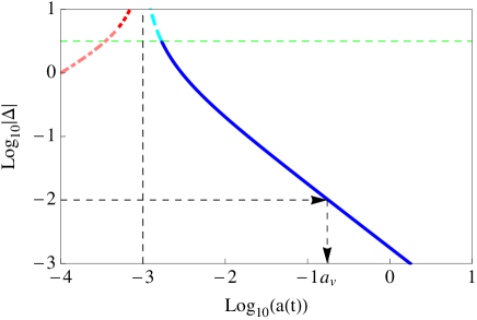
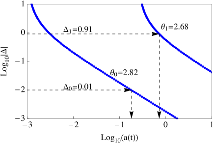
Figure 6 shows $R_{\Delta}(t)$ for $\theta=2.82$ and initial scale factor $a_{0}=10^{-3}$. All $\Delta$ yield expanding open models for this $\theta$; one choice corresponds to the model whose LPT series appeared in figure 1 ($\Delta=0.01$, $\theta=2.82$, $a_{0}=10^{-3}$). The x-axis is $\log a$ and is equivalent to a measure of time. The y-axis is $\log|\Delta|$, i.e. the distance from the origin to poles in the complex $\Delta$ plane. In principle, future evolution may be limited by real or complex roots. The blue solid line and the red dotted line indicate real and complex roots of $\eta=2\pi$ respectively. The cyan dashed and pink dot-dashed lines indicate the real and complex roots of $\eta=0$ respectively. Future evolution is constrained by real roots (blue and cyan) in this example.

The time of validity is the first instance when a singularity appears within the disk of radius $\Delta$ in the complex $\bm{\Delta}$ plane. For the specific case, starting at ordinate $\Delta=10^{-2}$, one moves horizontally to the right to intersect the blue line and then vertically down to read off the scale factor $a_{v}=a[T(\Delta)]=0.179$. The time of validity inferred from the root plot agrees quantitatively with the numerical results in figure 1.

Appendix D presents a comprehensive set of results. The time of validity is finite for any open model. As expected, smaller amplitudes imply longer times of validity. The poles do not correspond to collapse singularities reached in the course of normal physical evolution since the open models do not have any real future singularities. A hint of an explanation is already present, however. The green dashed line is $\delta_{v}=1$ (or $\Delta=1/\sin\theta$) at which point the root switches from $\eta=2\pi$ below to $0$ above. Such a switch might occur if varying the initial velocity transposes an expanding closed model into a contracting closed model. But it is expected to occur at $\delta_{v}=-1$ not $1$. The open models are apparently sensitive to past and future singularities in closed models with initial conditions that are transformed in a particular manner. §5.3 explores this interpretation in detail.

5.2 Closed models

Figure 7 presents $R_{\Delta}(t)$ for models with $\theta=0.44$ and $a_{0}=10^{-3}$. There are several new features. Over the angular range $\theta_{c}^{-}<\theta<\theta_{c}^{+}$ the cosmology is closed for small $\Delta$ (see shaded region in figure 2 near $\Delta=0$). Conversely, a straight line drawn from $\Delta=0$ within this angular range must eventually cross the parabola $E=0$ except for the special case $\theta=0$. Since the velocity contribution to energy $E\propto\Delta^{2}$ while the density contribution $\propto-\Delta$ it is clear that eventually $E>0$ as $\Delta$ increases. The critical value, $\Delta_{E=0}$, is a function of $\theta$. Below the brown horizontal dot-dashed line in figure 7 the models are closed, above they are open (line labelled $\Delta=\Delta_{E=0}$).

The root plot has, as before, blue solid and red dotted lines denoting the distance to real and complex $\bm{\Delta}$ poles, respectively, for $\eta=2\pi$. The cyan dashed line denotes real roots for $\eta=0$ and does not restrict future evolution.

Figure 7: $R_{\Delta}$ for $\theta=0.44$ and $a_{0}=10^{-3}$. The line $\Delta_{E}=0$ separates open and closed models. The scale factor at the time of validity is $a_{v}$. For closed models the scale factor at time of collapse is $a_{c}$. Blue solid line and red small dashed line denote real and complex roots of $\eta=2\pi$, respectively. The cyan dashed lines denotes the real roots of $\eta=0$. When the first singularity encountered is real, $a_{v}=a_{c}$, the time of validity is the future time of collapse. However, when the singularity is complex the time of validity is less than the actual collapse time. In the range $\Delta_{rc}<\Delta<\Delta_{E=0}$, there are closed models with $a_{v}<a_{c}$.

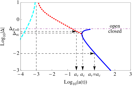
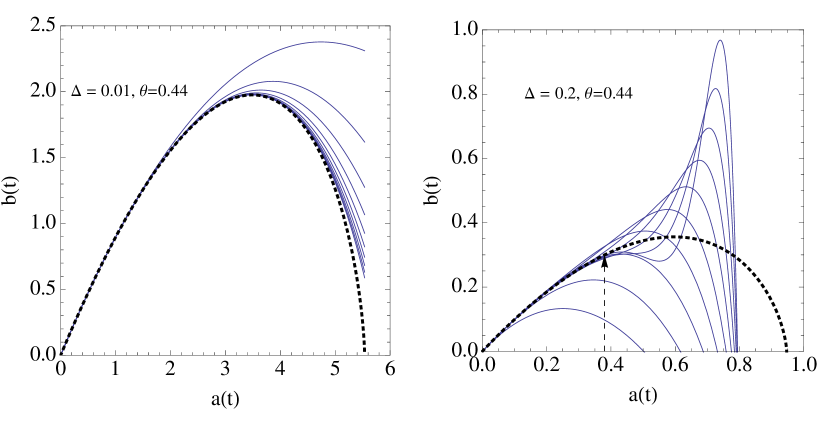
For small $\Delta$ real roots determine the time of validity. These roots correspond exactly to the model’s collapse time. In other words, the time of validity is determined by the future singularity. For example, for $\Delta=0.01$, the root plot predicts that a series expansion should be valid until the collapse at $a=5.5$ denoted by “$a_{v}=a_{c}$” on the x-axis . This prediction is confirmed in the left hand panel of figure 8. The root diagram is consistent with the qualitative expectation that small overdensities should have long times of validity because collapse times are long: $\lim_{\Delta\to 0}T(\Delta)\to\infty$.

As $\Delta$ increases from very small values, i.e. successively larger initial density perturbations, the collapse time decreases. Eventually the velocity perturbation becomes important so that at $\Delta=\Delta_{rc}$ a minimum in the collapse time is reached. For $\Delta_{E=0}>\Delta>\Delta_{rc}$ the collapse time increases while the model remains closed. As $\Delta\to\Delta_{E=0}$ the collapse time becomes infinite and the model becomes critical. All models with $\Delta>\Delta_{E=0}$ are open.

The root diagram shows that for $\Delta>\Delta_{rc}$, the time of validity is determined by complex not real $\bm{\Delta}$ for $\eta=2\pi$. Closed models with $\Delta_{rc}<\Delta<\Delta_{E=0}$ have a time of validity less than the model collapse time. For example, for $\Delta=0.2$, the collapse occurs at $a=0.94$ but convergence is limited to $a\leq 0.38$. This prediction is verified in the right panel of figure 8.

The convergence of LPT expansions for some closed models is limited to times well before the future singularity. This general behaviour is observed for $\theta_{c}^{-}<\theta<\theta_{c}^{+}$ and $\Delta_{rc}<\Delta<\Delta_{E=0}$ where both $\Delta_{rc}$ and $\Delta_{E=0}$ are functions of $\theta$. Appendix D provides additional details.

Figure 8: The exact solution (black, dashed) and LPT expansions of successively higher order (blue) for two expanding, closed models with $\theta=0.44$. The left hand panel has $\Delta=0.01$. LPT converges to the exact solution at all times up to the singularity at $a=5.5$. The right hand panel has $\Delta=0.2$. LPT does not converge beyond $a=0.38$.

5.3 Mirror models, real and complex roots

The parametrization of the perturbation in terms of $\Delta>0$ and $-\pi<\theta\leq\pi$ and the complexification of $\Delta\to\bm{\Delta}$ can give rise to poles anywhere in the complex $\bm{\Delta}$ space. When $R_{\Delta}$ is determined by a pole along the real positive axis, a clear interpretation is possible: the future singularity of the real physical model exerts a dominant influence on convergence. LPT expansions for closed models with $\Delta<\Delta_{rc}$ are limited by the future collapse of the model and are straightforward to interpret.

The meaning of real roots for open models is less clear cut. The roots determining $R_{\Delta}$ at large $t$ are negative real and small in magnitude. Negative $\Delta$ lies outside the parameter range for physical perturbations taken to be $\Delta>0$. Nonetheless the mapping ($\Delta,\theta$) $\to$ ($-\Delta,\theta\pm\pi)$ preserves ($\delta$, $\delta_{v}$) and the original equations of motion. The poles of the models with parameters $(\Delta,\theta)$ and $(\Delta,\theta\pm\pi)$ are negatives of each other. Let us call these “mirror models” of each other.

For infinitesimal $\Delta$ if the original model is open then the mirror model is closed. Figure 2 shows that the $\Delta_{E=0}$ line has some curvature (in fact, it is a parabola) whereas the mirror mapping is an exact inversion through $\Delta=0$. Small $\Delta$ points are mapped between open and closed; large $\Delta$ points may connect open models to other open models.

If the original model is open with limiting pole which is negative real of small magnitude then it corresponds to a future singularity of the closed mirror model. For example, the closed model with parameters $(\Delta=0.01,\theta=0.44)$ in the left panel of figure 8 and the open model with parameters $(\Delta=0.01,\theta=0.44-\pi)$ shown in the left panel of figure 9 are mirrors. The time of the validity of the open model equals the time to collapse of its closed mirror.

The notion of mirror models explains other features of the root diagrams. The time of validity of open models was previously discussed using figure 6 ($\theta=2.82$). The blue solid line indicated real roots. Such roots are the future singularities of closed mirror models lying in the fourth quadrant along $\theta=2.82-\pi=-0.32$. As $\Delta$ increases the sequence of mirror models crosses the $\delta_{v}=-1$ line (the horizontal dashed line) to become initially contracting cosmologies and, in our labelling, the future singularity switches from $\eta=2\pi$ to $\eta=0$. This explains the switch in root label from blue solid to cyan dashed seen in figure 6, which occurs at $\delta_{v}=1$ in the original model.

The symmetry of the mirroring is not limited to cases when $\bm{\Delta}$ is real. It applies for complex $\bm{\Delta}$, too. For example, the models in the right panels of figures 8 and 9 are mirrors of each other. Their time of validity is the same and determined by complex roots which are negatives of each other. These singularities are non-physical and have no interpretation in terms of the collapse of any model yet they limit the LPT convergence in the same way.

Figure 10 shows the areas of phase space where complex roots determine the time of validity in light red. The area within the parabola (light blue) contains closed models. Most of the light blue region has a time of validity determined by real roots, i.e. the time to the future singularity. The area with both light blue and red shading encompasses closed models with the unexpected feature that the time of validity is less than the time to collapse.

The area outside the parabola contains open models. The time of validity of the unshaded region is determined by real roots. The original observation of LPT’s non-convergence for an underdensity (Sahni & Shandarin 1996) is an example that falls in this region. For small amplitude perturbations the time of validity is simply related by mirror symmetry to the occurrence of future singularities of closed models. The right hand plot in figure 9 is an example of an open model with time of validity controlled by complex roots (red shading outside the parabola).

Finally, some open models (especially those with large $\Delta$) have mirrors that are open models. Figure 11 shows mirror models ($\Delta=2$, $\theta=17\pi/36$) and ($\Delta=2$, $\theta=17\pi/36-\pi$). These are initially expanding and contracting solutions respectively. The root plot in figure 12 predicts that the series is valid until $a_{v}=0.0016$. The real root with $\eta=0$ (cyan line) sets the time of validity and corresponds to the bang time (the future singularity) of the initially contracting model.

Figure 9: Mirror models of the closed models of figure 8. Each graph shows the exact solution (black, dashed) and the LPT expansion to successively higher orders (blue) of one mirror model. The original model and the mirror have the same time of validity for the LPT expansion.

Figure 10: The red shaded region denotes part of phase space where complex roots play a role. The solid blue line represents the initial conditions which correspond to the background and perturbation having the same big bang time. The black solid parabola separates the closed and open models. Coloured version online.

Figure 11: Two open models which are mirrors of each other. Each plot shows the exact solution (black, dashed) and the LPT series expansion to successively higher orders (blue). The left panel is an initially expanding, open model whose convergence is limited to scale factors less than $a_{v}=0.0016$ (arrow). The right panel shows the initially contracting mirror model whose bang time at $a_{v}=0.0016$ is responsible for the limitation.

Figure 12: $R_{\Delta}$ for $\theta=17\pi/36$ and $a_{0}=10^{-3}$. The blue solid and cyan dashed lines denoted real roots with $\eta=2\pi$ and $\eta=0$ respectively. For $\Delta=2$, the time of validity is set by the root with $\eta=0$, which is the bang time of the mirror model with $\theta=17\pi/36-\pi$. See figure 11 for the evolution of both models.

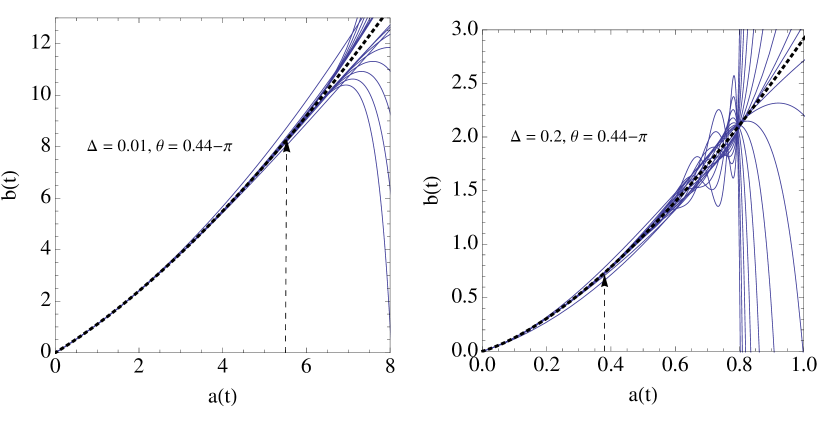
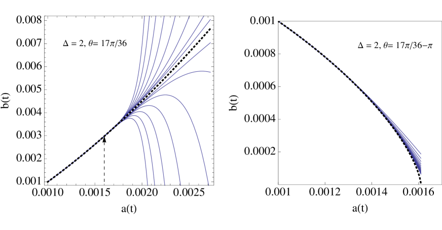
In all cases, the analysis correctly predicts the convergence of the LPT series.

5.4 Zeldovich and equal bang time models

The large expanse of phase space shaded light red in figure 10 suggests that complex roots should play a ubiquitous role in LPT applications but the situation is somewhat more subtle. For good physical reasons purely gravitational cosmological calculations often start with expanding, small amplitude, growing modes at a finite time after the big bang. The absence of decaying modes implies that the linearized perturbations decrease in the past . A non-linear version of this condition is that the perturbation amplitude is exactly zero at $t=0$. The same condition can be formulated as “the background and the perturbation have the same big bang time” or “the ages of the perturbation and the background are identical.” The condition is

$$\frac{1}{H_{0}}\int_{y=0}^{y=1}\frac{dy}{\left[(1+\Delta\cos\theta)y^{-1}+E(\Delta,\theta)\right]^{1/2}}=\frac{2}{3H_{0}}.$$ (41)

This is a nonlinear relationship between the two initial parameters $\Delta$ and $\theta$ which is shown by a thick blue line on the phase space diagram in figure 10. We have adopted the name “Zeldovich” initial conditions for the top-hat models that satisfy the equal bang time relation. There are a variety of definitions for Zeldovich initial conditions given in the literature. Generally, these agree at linear order. This one has the virtue that it is simple and easy to interpret. Note that the blue curve does not intersect the region of phase space where complex roots occur except, possibly, near $\bm{\Delta}=0$.

In the limit of small $\Delta$ eq. (41) becomes

$$\Delta(3\sin\theta-\cos\theta)=0.$$ (42)

The solutions are $\theta=\theta_{Z\pm}$ where $\theta_{Z+}=2.82$ and $\theta_{Z-}=\pi-\theta_{Z+}=-0.32$. The second quadrant solution $\theta_{Z+}$ corresponds to open models while its mirror in the fourth quadrant $\theta_{Z-}$ to closed models. Only when $\Delta\to 0$ can complex roots approach the loci of Zeldovich initial conditions but they intersect only in the degenerate limit.

In the next section, we will show that points starting close to the Zeldovich curve continue to stay near it as they move through phase space. Such models have real, not complex, roots. This implies that closed systems along the curve always have a convergent series solution. Hitherto, LPT convergence has been studied only for initial conditions close to the Zeldovich curve. This is why problems have been noted only in the case of voids. The existence of the complex roots is a new finding. All of the above is based on the spherical top-hat model which has a uniform density.

As emphasized above, there are good physical motivations for adopting Zeldovich-type initial conditions. The fact that cosmological initial conditions must also be inhomogeneous (i.e. Gaussian random fluctuations) is not captured by the top-hat model. One can imagine two extreme limiting cases for how the simple picture of top-hat evolution is modified. If each point in space evolves independently as a spherical perturbation then at any given time one expects to find a distribution of points along the Zeldovich curve. As time progresses this distribution moves such that the underdense points cluster around the attracting point $(-1,0.5)$ and overdense points move towards collapse. The distribution of initial density and velocity perturbations yields a cloud of points in phase space but complex roots never play a role because nothing displaces individual points from the Zeldovich curve. Each moves at its own pace but stays near the curve. Alternatively, it is well known that tidal forces couple the collapse of nearby points. These interactions amplify the initial inhomogeneities leading to the formation of pancakes and filaments. As time progresses motions transverse to the Zeldovich curve will grow. If these deviations are sufficient they may push some points into areas with complex roots. In a subsequent paper, we will explore these issues for general inhomogenous initial conditions.

6 LPT re-expansion

To overcome the constraints above, an iterative stepping scheme that respects the time of validity is developed for LPT. The initial parameters at the first step determine the solution for some finite step size. The output at the end of the first step determines the input parameter values for the next step and so on.

6.1 The Algorithm

Choose the background ($a_{0}$, $H_{0}$, $\Omega_{0}=1$, $Y_{0}$) and the perturbation ($b_{0}=a_{0}$, $H_{p0}$, $\Omega_{p0}$, $X_{0}$) at initial time $t_{0}$. The perturbed model is fully characterised by $H_{p0}$ and $\Omega_{p0}$ or by $\delta_{0}=\rho_{p0}/\rho_{0}-1$ and $\delta_{v,0}=H_{p0}/H_{0}-1$ or by $\Delta_{0}$ and $\theta_{0}$. Extra subscripts have been added to label steps.

LPT converges for times $t<T(\Delta_{0},\theta_{0})$. Use LPT to move forward to time $t_{*}$ satisfying $t_{0}<t_{*}<T(\Delta_{0},\theta_{0})$. At $t_{*}$, the background and perturbed scale factors and time derivatives are $a_{*}$, $b_{*}$, ${\dot{a}}_{*}$, and ${\dot{b}}_{*}$. The fractional density and velocity perturbations with respect to the background are

$$\delta_{*} = (1+\delta_{0})\left(\frac{a_{*}}{b_{*}}\right)^{3}-1$$ (43)

$$\delta_{v,*} = \frac{{\dot{b}}_{*}/b_{*}}{{\dot{a}}_{*}/a_{*}}-1.$$ (44)

Re-expand the perturbation around the background model as follows. First, let the time and Lagrangian coordinate for the background (inner edge of the unperturbed sphere) be continuous: $t_{1}=t_{*}$ and $Y_{1}=Y_{0}$. These imply $a_{1}=a_{*}$ and ${\dot{a}}_{1}={\dot{a}}_{*}$, i.e. the scale factor and Hubble constant for the background are continuous.

At the beginning of the first step we assumed $a_{0}=b_{0}$. This is no longer true at the end of the first step. Define a new Lagrangian coordinate $X_{1}=X_{0}b_{*}/a_{*}$, new scale factor $b_{1}=a_{*}$, and new scale factor derivative ${\dot{b}}_{1}={\dot{b}}_{*}a_{*}/b_{*}$. These definitions leave the physical edge of the sphere and its velocity unaltered

$$r_{physical,*} = b_{*}X_{0}=b_{1}X_{1}$$ (45)

$${\dot{r}}_{physical,*} = {\dot{b}}_{*}X_{0}={\dot{b}}_{1}X_{1}.$$ (46)

The re-definitions relabel the fluid elements with a new set of Lagrangian coordinates and re-scale the scale factor. The perturbation parameters are unchanged $\delta_{1}=\delta_{*}$ and $\delta_{v,1}=\delta_{v,*}$ because physical quantities are unmodified. Consequently, $\Delta_{1}=\Delta_{*}$ and $\theta_{1}=\theta_{*}$.

6.2 Flow dynamics in the phase space

To examine how Lagrangian re-expansion works consider how the Lagrangian parameters $\Delta$ and $\theta$ would vary if they were evaluated at successive times over the course of a specific cosmological history. Let $\delta(t)$ and $\delta_{v}(t)$ be defined via eq. (3) and apply the second-order equations of motion eqs. (9) and (10) to derive the coupled first-order system

$$\frac{d\delta}{dt} = -\frac{2}{t}\delta_{v}(1+\delta)$$ (47)

$$\frac{d\delta_{v}}{dt} = \frac{1}{3t}\left\{(1+\delta_{v})(1-2\delta_{v})-(1+\delta)\right\}$$ (48)

where all occurrences of $\delta$ and $\delta_{v}$ are functions of time. From $\delta(t)$ and $\delta_{v}(t)$ one infers the parameters, $\Delta(t)$ and $\theta(t)$. These have the following simple interpretation: a Lagrangian treatment starting at time $t^{\prime}$ has $\Delta=\Delta(t^{\prime})$ and $\theta=\theta(t^{\prime})$ in the LPT series.

Since the system is autonomous it reduces to a simple flow in phase space. The flow has three fixed points at $(\delta,\delta_{v})=(0,0)$, the unperturbed, background model, $(-1,-1)$, a vacuum static model, and $(-1,0.5)$, a vacuum expanding model. Linearizing around $(0,0)$ shows it is a saddle fixed point. The tangent to the $E=0$ curve at the origin is the attracting direction and the tangent to the equal big bang curve is the repelling direction. The fixed point at $(-1,0.5)$ is a degenerate attracting node and that at $(-1,-1)$ is an unstable node. The flow vectors are plotted in the left panel of figure 13. The blue shaded region indicates closed models and red shaded region indicates models where complex roots limit the time of validity for LPT.

Note that the flow lines smoothly cover the whole phase space. The interpretation is that the continuous relabelling of Lagrangian coordinates and re-scaling of the scale factor has the potential to overcome the convergence limitations discussed thus far. Otherwise one might have seen ill-defined or incomplete flows or flows that were confined to a given region.

Figure 13: The left panel shows streamlines of the flow described by eq. (48). The colour coding of the plot is same as figure 10. The right panel zooms in on the area near the origin which is where all models are located at sufficiently early times. At late times, open models move away from the origin towards the attracting fixed point at $(\delta,\delta_{v})=(-1,0.5)$. The attraction to the Zeldovich solution is shown for a set of initial conditions (yellow, cyan, green and black lines) that begin near but not on the critical trajectory. Closed models move out to infinity along the fixed big bang time curve. Coloured version online.

6.2.1 Asymptotic limits of open and closed models

The right panel of figure 13 zooms in on the area near the origin. Initial points that correspond to open models starting near the origin approach the Zeldovich curve and asymptotically converge to the strong attractor at $(\delta,\delta_{v})=(-1,0.5)$.

Closed models collapse and the density $\delta\rightarrow\infty$. In the asymptotic limit, the solution to (48) is given by $\delta\sim\delta_{v}^{2}+K$ with integration constant $K$. From figure 13, the flow lines of closed models that start in the vicinity of the origin trace a parabolic path that is parallel and essentially equivalent to the Zeldovich curve.

The flow shows where re-expansion is needed. Closed model flow lines that start near the origin never pass through the red shaded region where complex roots play a role; the time of validity equals the time to collapse and no re-expansion is needed. However, closed models that originate in the red region must be re-expanded. The flow suggests that they eventually move into the blue region. So even though a closed model may initially have an LPT series with limited convergence, re-expansion makes it possible to move into the part of phase space where a single step suffices to reach collapse.

6.3 Finite steps and feasibility

This section and the next examine the feasibility of extending a solution from recombination to today. The results will be applied to fully inhomogeneous evolution in future paper.

Let the asymptotic time of validity for an open model be expressed in dimensionless form $\chi=\lim_{t\to\infty}H(t)T(\Delta(t),\theta(t))$. Here, $\Delta\to\sqrt{5/4}$ and $\theta\to\tan^{-1}(-1/2)=2.677$ and $T(\Delta,\theta)$ is determined by the future time to collapse of the closed mirror model. The result is $\chi=2.62$ (numerical results in Appendix D), the time of validity is proportional to the characteristic age of the background and individual steps grow larger and larger.

An example shows that the basic effect can be seen even before the asymptotic regime is achieved. Figure 14 sketches the first two steps where the assumed model parameters at the first step are $(\Delta_{0},\theta_{0})=(0.01,2.82)$. The scale factor at the time of validity is $a=0.179$. A step with half the allowed increment in time is taken and the system is re-initialised. The re-initialisation implies ($\Delta_{1},\theta_{1})=(0.91,2.68)$ or $(\delta_{1},\delta_{v,1})=(-0.82,0.4)$. Afterwards the new time of validity is larger in this example.

Figure 14: Extending the time of validity of LPT. The first step has $\Delta_{0}=10^{-2}$ and $\theta=2.82$ and implies scale factor at the time of validity $a_{v}=0.179$. Incrementing by half the allowed step gives initial conditions for the second step $(\Delta_{1},\theta_{1})=(0.91,2.68)$. Note that the new time of validity has increased.

The feasibility of the re-expansion scheme can be examined by evaluating the ratio of the time of validity before ($T$) and after ($T^{\prime}$) a step

$$\alpha=\frac{T^{\prime}}{T}.$$ (49)

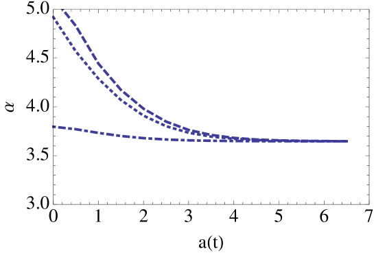
Figure 15 shows $\alpha$ evaluated along the continuous flow as a function of scale factor for three different starting initial conditions. Since $\alpha>3$ at all times, starting at initial time $t_{i}$ the time after $N$ steps is roughly $t\sim\alpha^{N}t_{i}>3^{N}t_{i}$.

Consider, for example, the number of steps needed to extend an open solution from recombination to today. Let $t_{f}$ ($t_{i}$) be the final (initial) time of interest where $t_{f}/t_{i}\sim a_{f}/a_{i}\sim 10^{4.5}$. Estimating $\alpha=3$ implies $N\sim\log_{3}10^{4.5}\sim 10$ steps are needed. This numerical result for $N$ is an overestimate and one can do better. It is important to recall that it based on an arbitrarily high order expansion which achieves an exact solution. If one is limited to calculations of finite Lagrangian order and imposes a maximum numerical error at the end of the calculation then more than $N$ steps may be required. At least $N$ steps are needed for series convergence and more than $N$ steps may be needed for error control.

One can extend any open model to an arbitrary future time while respecting the time of validity of the LPT series. The number of steps is governed by a geometric progression.

One can also extend any closed model to the future singularity while respecting the time of validity of the LPT series. Only a single step is needed for a closed model when the root is real (blue shaded region of figure 13). When it is complex (the region shaded both blue and red) the model flows first toward the node at $(0,0)$ ($\Delta$ decreases) and ultimately reaches the region of real roots. Multiple steps will generally be necessary to escape the region of complex roots. An approximate fit (eq. (88)) shows that $\chi\sim T(\Delta,\theta)H(t)\propto\Delta^{\beta}$ for small $\Delta$ where $\beta<-2.5$. Both $\chi$ and the time of validity increase as the node is approached. Time advances at least as quickly as a geometric progression and this is analogous to the manner in which the open model steps towards its limit point. However, unlike the open case, once the trajectory crosses into the blue region (assuming it does not lie exactly on the unstable attracting trajectory) a single final step is needed. The specific number of steps will depend upon the starting initial conditions but will be small because of the property of geometric progression.

Figure 15: The ratio of successive times of validity ($\alpha$) vs. $a(t)$. The dashed, dot-dashed and dotted lines indicate three initial starting points $(0.5,0.5),(0,1),(-0.2,0.2)$ respectively. The ratio converges to about 3.6 and the time of validity increases geometrically with $N$.

6.4 Demonstrative examples

LPT re-expansion can solve the problematic convergence in previously analysed open and closed models.

Open models have asymptotic values of $\Delta$ and $\theta$ and simple evolution. The first section below includes numerical results that provide a practical demonstration of the success of LPT re-expansion in this case. Convergence as Lagrangian order increases and/or time step size decreases is observed qualitatively.

Closed models have a somewhat more complex behaviour (before and after turnaround). The second section provides both a qualitative and quantitative discussion of convergence. The scaling of the leading order error and the time step control which are derived are of general applicability.

6.4.1 Open model

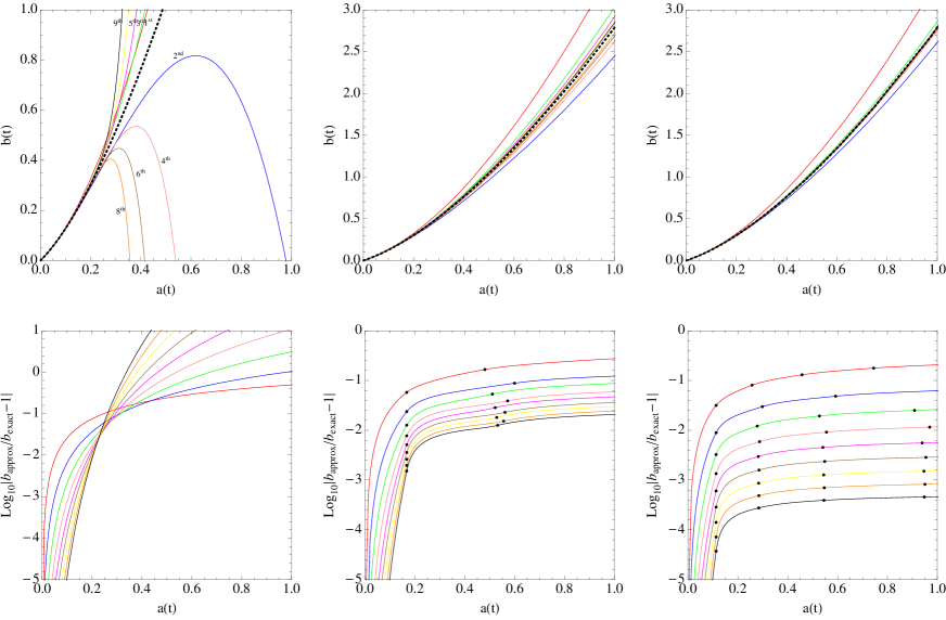
Figure 16 investigates the effect of time step and order on the evolution of the open model introduced in figure 1 ($\Delta=0.01$, $\theta=2.82$, $a_{0}=10^{-3}$). The series convergence breaks down at $a=0.179$. The left panel shows an attempt to take a single step to $a=1$ using successively higher LPT series orders. As expected, higher order terms do not improve the accuracy of the description because the time of validity is violated. The middle panel employs three steps to reach $a=1$, each respecting the time of validity. Now the LPT series with higher order improves the accuracy just as one desires. The right panel employs six steps to reach $a=1$, each respecting the time of validity. Again, higher order improves the description. Note that more frequent re-expansion, i.e. smaller steps in time, improve the errors at fixed LPT order.

Figure 16: LPT re-expansion of an open model with $\Delta_{0}=0.01$ and $\theta_{0}=2.82$. The top three figures show the scale factor for the same initial conditions calculated with one step (left), three steps (middle) and five steps (right). The black dots indicate the position of the time steps. In the middle and right panels, the solution was advanced $9/10$ and $1/2$ the allowed time of validity, respectively. The bottom figures show the errors for all LPT approximations to $b(t)$ including the unphysical negative ones. The order of the LPT expansion are colour-coded according the top left figure. The single step expansion does not respect the time of validity whereas both the three and six step examples do. The original expansion does not converge over the full time range whereas the re-expansions do. Coloured version online.

6.4.2 Closed model

Figure 17 investigates the closed model introduced in figure 8 ($\Delta=0.2,\theta=0.44,a_{0}=10^{-3}$). The time of validity is determined by a complex root. The first panel shows that the series begins to diverge at $a=0.38$ well before the collapse singularity is reached at $a=0.94$.

A single time step less than the time of validity is guaranteed to converge as the order of the Lagrangian expansion increases. LPT re-expansion utilises a set of such time steps each of which is likewise guaranteed to converge. However, since a calculation of infinite order is never achieved in practice, it is worth characterising how convergence depends upon two calculational choices one has at hand, the time step and the order of the Lagrangian expansion.

A single small step beginning at $t=t_{0}$ and ending at $t_{f}$ has leading order error for the $m$-th order Lagrangian approximation $\propto(t_{f}/t_{0}-1)^{m+2}\Delta^{m+1}$, where $\Delta$ is the value at the initial time. If the same small interval is covered in $N$ smaller steps, the error after $N$ steps scales as $N^{-m}(t_{f}/t_{0}-1)^{m+2}\Delta^{m+1}$ (see Appendix E for details). If the step size increases in a geometric sequence such that $\delta t/t$ is a constant for each intermediate step, then $t_{f}=t_{0}(1+\delta t/t)^{N}$ and the error after $N$ steps scales as $N(t_{f}/t_{0}-1)(\delta t/t)^{m+1}\Delta^{m+1}$. This leads to the interpretation that the error per intermediate step scales as $(\delta t/t)^{m+1}\Delta^{m+1}$. Define $\epsilon=(\delta t/t)\Delta$. The leading order error scales as $\epsilon^{m+1}$ which is numerically small if $\epsilon<1$. The sum of all the missing higher order terms is finite if $\delta t<T$, i.e respects the time of validity.

In a practical application, the initial and final times are not close. A reasonable time step criterion is to choose $\epsilon<1$ fixed throughout the evolution and to infer $\delta t$ for a given $\Delta$. Other choices are possible but $\delta t$ must always be less than the time of validity. If $\epsilon$ is held fixed throughout the evolution, then the net error after $N$ steps for the $m$-th order approximation $\propto\epsilon^{m+1}N$.

The number of steps required to go from the initial to the final time can be estimated. As a special case assume that $\Delta$ is constant. The time step criterion implies that the number of steps to move from the initial time $t=t_{0}$ to the final time $t_{f}$ for given $\epsilon$ is $N=\log(t_{f}/t_{0})/\log(1+(\epsilon/\Delta))$. For limited total intervals ($t_{f}-t_{0}<<t_{0}$) and small steps ($\epsilon/\Delta<<1$) the exact answer reduces to $N\sim(t_{f}-t_{0})\Delta/\epsilon=(t_{f}-t_{0})/\delta t$. Here $\delta t=\epsilon t\Delta$ does not grow appreciably over the interval so the estimate for $N$ is a maximum. In this limit, the net error $\propto\epsilon^{m}\Delta$. The leading order error for the m-th order Lagrangian scheme decreases at least as quickly as $\epsilon^{m}$.

In more general situations the value of $\Delta$ varies. Once the closed model turns around $\Delta$ increases without bound. For fixed $\epsilon$ the step size $\delta t$ decreases monotonically to zero as $t\to t_{coll}$ where $t_{coll}$ is the time of the future singularity. At any order it would take infinitely many steps to follow the solution up until collapse. Consider the problem of tracking the solution up to a large, finite value of $\Delta=\Delta_{f}$. This moment corresponds to a fixed time $t_{f}\mathbin{\lower 3.0pt\hbox{$\hbox to0.0pt{\raise 5.0pt\hbox{$\char 60\relax$}\hss}\mathchar 29208\relax$}}t_{coll}$ in the exact solution. The number of steps $N<N_{max}\sim t_{f}/\delta t_{f}$ where $\delta t_{f}$ is the step size for the system near $\Delta_{f}$; $\delta t_{f}\propto\epsilon/\Delta_{f}$. The leading order error after $N$ steps at the $m$-th Lagrangian order $\propto\epsilon^{m+1}N<\epsilon^{m+1}N_{max}\sim\epsilon^{m}\Delta_{f}$. This method of step control forces the leading order error at fixed time $t_{f}<t_{coll}$ to decrease as the Lagrangian order $m$ increases and/or the control parameter $\epsilon$ decreases.

The second and third panels in figure 17 show the runs with $\epsilon=0.5$ and $\epsilon=0.2$ respectively. The Lagrangian orders are colour-coded; dots show time steps determined by the above criterion. At each order the solution was terminated when the numerically determined $\Delta>100$ so as to avoid the infinite step regime. This required 32 steps for the $\epsilon=0.5$ run and 77 steps for the $\epsilon=0.2$ run. As the red solid lines illustrates, the first order solution turns around before all other solutions. This explains why its step size begins to shrink near the midpoint of the graph. By contrast, all the step sizes for higher order solutions are very similar up to that point.

The numerical errors may be analysed from two points of view.

1. A comparison of different coloured lines (different Lagrangian orders) in a single panel shows that error decreases as $m$ increases. This is true in a quantitative as well as qualitative sense. For example, in the second panel at $a=0.64$ a plot of the log of the absolute error is approximately linear in $m$, as expected.

2. A comparison of the same coloured lines in the middle and right panels shows that smaller $\epsilon$ implies better accuracy. Again, this is true in a quantitative as well as qualitative sense. For example, the observed ratio of errors at $a=0.64$ for the $9$-th order calculations is $5\times 10^{-4}$. To evolve up to this time with $\epsilon=0.5$ (middle panel) takes 10 steps; with $\epsilon=0.2$ (right panel) it takes 22 steps. The expected ratio of errors is $(0.2/0.5)^{9+1}(22/10)\sim 2\times 10^{-4}$, the same order of magnitude as the observed ratio.

These comparisons lead to the important conclusion that the leading order error for LPT re-expansion varies with Lagrangian order and time step as theoretically expected.

It is clear that considerable benefit accrues not only from implementing higher order Lagrangian schemes but also by limiting time step size (which must always be less than the time of validity). For simple examples like the top-hat it is feasible to work to very high Lagrangian order but this is not likely to be true in the context of more complicated, inhomogeneous problems. On the other hand, marching forward by many small time steps using LPT re-expansion is generally feasible. In the example above the initial perturbation is $\Delta=0.2$ whereas a practical calculation starting at recombination would start with $\Delta\sim 10^{-5}$. For the same $\epsilon$ the practical application requires more steps for the phase before turnaround but the net increase is only a modest logarithmic factor. In fact, most of the steps in the example were taken after turnaround and the total number varies with the depth of the collapse. This will continue to be true for the practical calculation. The choice of step size and order for such applications will be the subject of a forthcoming paper.

Figure 17: LPT re-expansion of a closed solution with $\Delta=0.2$, $\theta=0.44$. The top three figure show the scale factor calculated with a single step (left) and multiple steps with $\epsilon=0.5$ (middle) and $\epsilon=0.2$ (right) (refer to text for definition of $\epsilon$). The bottom figures show the errors for all LPT approximations to $b(t)$ including the unphysical negative ones. The order of the expansion is colour-coded as in the top left figure. The single step expansion does not respect the time of validity whereas both the other cases do. The black dots indicate the position of the time steps. The original expansion does not converge over the full time range whereas the re-expansions do. Coloured version online.

7 Conclusion

We have investigated the time of validity of Lagrangian perturbation theory for spherical top-hat cosmologies with general initial conditions. Using techniques from complex analysis we showed that the time of validity is always limited for open models. We also discovered a class of closed models whose time of validity is less than their time to collapse. We introduced the concept of the mirror model and derived a symmetry principle for the time of validity of mirror models. For small initial perturbations the time of validity of LPT series expansion of an open model corresponds to the collapse time of a closed mirror model.

A qualitative analogy is useful. A single LPT series expansion is similar to a single step in a finite difference approximation for advancing a hyperbolic partial differential equation like the wave equation. The time of validity of the LPT expansion is analogous to the Courant condition which guarantees stability. In LPT the constraint is an acceleration-related time-scale; in the wave equation it is a sound-crossing time-scale.

We developed the method of LPT re-expansion which overcomes the limitations intrinsic to a single expansion. We demonstrated how to iteratively re-expand the solution so as to link convergent series expressions that extend from initial to final times. The time of validity of the expansions set the minimum number of re-expansion steps ($\sim 10$) necessary for cosmological simulations starting at recombination and proceeding to the present epoch. Finite as opposed to infinite order Lagrangian expansions required extra steps to achieve given error bounds. We characterised how the leading order numerical error for a solution generated by LPT re-expansion varied with the choice of Lagrangian order and of time step size. We provided a recipe for time step control for LPT re-expansion based on these results.

Our long-term goal and motivation for this study is to develop a numerical implementation of LPT re-expansion for fully inhomogeneous cosmological simulation. Top-hats with Zeldovich initial conditions have special properties with respect to LPT convergence. We found that all underdense models must be treated by re-expansion while none of the overdense ones need be. However, during the course of an inhomogeneous simulation the density and irrotational velocity perturbations (with respect to a homogeneous background cosmology) at an arbitrary point will generally not fall on the top-hat’s Zeldovich curve. Hence, the convergence of LPT in inhomogeneous applications must be guided by the analysis of more general models. Top-hats with arbitrary initial conditions are the simplest possibility and constitute the main focus in this paper. The limitations on LPT convergence which we have elucidated in this generic case are considerably more complicated than in the top-hat with Zeldovich initial conditions. Our plan is to use the generic time of validity criterion to determine the time-stepping for inhomogeneous evolution. This should allow us to develop high-precision simulations with well-defined control of errors. The practical impact of a refined treatment of LPT convergence is not yet clear.

The convergence issues we have dealt with should not be confused with the breakdown when orbit crossing takes place and the Jacobian of the transformation from Lagrangian to physical coordinates becomes singular. At that time the flow becomes multi-streamed and much of the simplicity and advantage of the Lagrangian approach vanishes. The aim of the current work is to make sure it is possible to reach the epoch of multi-streamed flow but offers nothing new on how to proceed beyond it. In fact, it may be necessary to include an effective pressure term in the equations to account for the velocity dispersion induced by orbit crossing (Adler & Buchert 1999; Buchert, Dominguez & J.Perez-Mercader 1999) or to adopt alternative approximations for the basic dynamics (such as the adhesion approximation; see Sahni & Coles 1995 for a review and references therein) to make progress.

Appendix A Formal set-up of the spherical top-hat

We intend to study an inhomogeneous universe. It contains a single, compensated spherical perturbation evolving in a background cosmology. To describe two spatially distinct pieces of the inhomogeneous universe (the background and the central perturbation) we invoke the language of homogeneous cosmology.

A.1 Description of the background

The origin of the coordinate system is the centre of the sphere. The background system at the initial time $t_{0}$ is set by the physical size of the inner edge $r_{b,0}$, the velocity ${\dot{r}_{b,0}}$ and density parameter $\Omega_{0}$. The Lagrangian coordinate system is extended linearly throughout space once the Lagrangian coordinate of the inner edge is fixed. Let the Lagrangian coordinate of the inner edge be

$$Y=\frac{r_{b,0}}{a_{0}}.$$ (50)

Either choose the initial background scale factor $a_{0}$ and determine the coordinate system or, alternatively, fix $Y$ and infer the background scale factor. In either case, the scale factor embodies the gauge freedom associated with the radial coordinate system.

The future evolution of the inner edge of the background is given by $r_{b}(t)=a(t)Y$. The velocity at the initial time satisfies ${\dot{r}}_{b,0}=\dot{a}_{0}Y$. The density at any later time is

$$\rho_{b}(t)=\frac{\rho_{b0}a_{0}^{3}}{a^{3}},$$ (51)

and the Hubble parameter for the background is

$$H_{0}=\frac{{\dot{r}}_{b,0}}{r_{b,0}}=\frac{{\dot{a}}_{0}}{a_{0}}.$$ (52)

The evolution of the scale factor is

$$\frac{{\ddot{a}}}{a}=-\frac{4\pi G\rho_{b0}a_{0}^{3}}{a^{3}}=-\frac{1}{2}\frac{H_{0}^{2}a_{0}^{3}\Omega_{0}}{a^{3}}$$ (53)

The quantities, $r_{b,0}$, ${\dot{r}}_{b,0}$, $\Omega_{0}$ and $t_{0}$ along with the choice of the coordinate system, completely specify the background universe.

A.2 Description of the innermost perturbation

The perturbation can be described by four physical quantities: the physical position $r_{p,0}$ and velocity ${\dot{r}}_{p,0}$ of the edge (or the ratio $H_{0p}={\dot{r}}_{p,0}/r_{p,0}$), the density parameter $\Omega_{p0}$ at the initial time $t_{0}$. The Lagrangian coordinate system for the perturbation is

$$X=\frac{r_{p,0}}{b(t_{0})}.$$ (54)

It can be linearly extended throughout space.

Like $a_{0}$, $b(t_{0})$ embodies the gauge freedom associated with the choice of the coordinate system. Without loss of generality, one can pick this gauge to satisfy

$$b(t_{0})=a_{0}.$$ (55)

Note that the Lagrangian coordinate systems for the background and perturbation are different.

Let $\rho_{0}$ and $\rho_{p,0}$ denote the densities of the background and perturbation respectively. Define the perturbation parameters

$$\delta = \frac{\rho_{p0}}{\rho_{b0}}-1$$ (56)

$$\delta_{v} = \frac{H_{0p}}{H_{0}}-1$$ (57)

giving

$$\Omega_{0p}=\frac{(1+\delta)}{(1+\delta_{v})^{2}}.$$ (58)

A.3 Inhomogeneous model

Figure 18: A cartoon showing the physical set-up of the problem.

Figure 18 shows how an overdense and underdense innermost sphere may be embedded with compensation in a homogeneous background universe. The assumption that the background cosmology evolves like a homogeneous model, fully described in terms of its Hubble constant and density, imposes consistency conditions. At the initial instant the “inner edge” of the unperturbed background distribution is at physical distance $r_{b,0}$ from the centre of the sphere. The region with $r>r_{b,0}$ will evolve like an unperturbed homogeneous cosmology as long as

1. the mass within equals the mass that an unperturbed sphere would contain;

2. matter motions within the perturbed region do not overtake the inner edge of the homogeneous region.

These conditions which are obvious in the Newtonian context have general relativistic analogues (Landau & Lifshitz 1975).

Next, consider the innermost perturbed spherical region. At the initial time let $r_{p,0}$ be the “outer edge” of this region. The physical properties and evolution of the innermost region are fully described in terms of its Hubble constant and density as long as its outer edge does not overtake matter in surrounding shells. While this is obvious in a Newtonian context there exists a relativistic analogue (Tolman 1934; Landau & Lifshitz 1975).

The inhomogeneous model is incomplete without specification of the transition region between the innermost sphere and the background. For the background to evolve in an unperturbed fashion the mass within $r_{b,0}$ must be exactly $4\pi\rho_{0}r_{b,0}^{3}/3$. There are many ways to satisfy this requirement. For example, when $\delta>0$ a simple choice is to place an empty (vacuum) shell for $r_{p,0}<r<r_{b,0}$ so that $(\rho_{p0}/\rho_{0})=(r_{b,0}/r_{p,0})^{3}=(Y/X)^{3}$. The evolution of each matter-filled region proceeds independently as long as the trajectories of the inner and outer edges do not cross. When $\delta<0$, a more complicated transition is required. For example, one choice is to nest sphere, empty shell and dense shell (see figure 18) so that the mass within $r_{b,0}$ matches that of the unperturbed background. In this case $\rho_{p0}r_{p,0}^{3}=f\rho_{0}r_{b,0}^{3}$ for some $f<1$ (the remaining fraction $1-f$ is placed in the dense shell). Varying the specifics of the compensation region while keeping the properties of the sphere fixed leaves $\delta$ and $\delta_{v}$, as defined above, invariant.

For fixed $\delta$ and $\delta_{v}$ the solution $b(t)$ is independent of the details of the transition. Nonetheless, variation in $f$, $r_{b,0}/r_{p,0}$ and $Y/X$ all go hand-in-hand. Hence, the extent of time that the sphere’s evolution may be treated as independent of the matter-filled outer regions also varies. A basic premise of this paper is that it is meaningful to determine the limitations arising from the convergence of the LPT series independently of limitations associated with crossing of separate matter-filled regions. For a given a $\delta$ and $\delta_{v}$ this separation can be achieved for specific constructions by choosing the radius and (hence velocity) of the inner sphere and the energy of the compensating region appropriately.

A.4 Number of degrees of freedom for the innermost sphere

If the innermost sphere corresponds to an overdensity then the compensating region can be a vacuum as shown in figure 18. Having picked the co-ordinate system, having selected equal initial times for the background and perturbation (not equal bang times but equal times at which we give the background and perturbation values), and required the correct amount of mass, only two degrees of freedom remain: $\delta$ and $\delta_{v}$.

To reiterate, the background and the perturbation can have different big bang times. Setting them equal would imply a relationship between $\delta$ and $\delta_{v}$ and leave a single free parameter.

If the innermost sphere corresponds to an underdensity then the compensating region is not vacuum but a spherical shell. In this case, in addition to $\delta$ and $\delta_{v}$, one must specify $f$ or, equivalently, $r_{p,0}$. But the solution for $b(t)$ is independent of the size of the innermost sphere so, again, only two degrees of freedom remain.

A.5 Preventing shell crossing

There are two sorts of limitations for the solution of $b(t)$. One is the calculation-dependent limitation arising from the convergence properties of the Lagrangian series expansion. It involves the scale factors only. The other is a physical limitation arising from collisions of the innermost region with surrounding non-vacuum regions (either the background or a compensating shell). We show that it is possible to delay the epoch of collisions indefinitely without altering the evolution of the innermost region.

Fix $H_{0}$, $H_{p,0}$, $\rho_{0}$ and $\rho_{p,0}$. This implies that the expansion parameters in LPT, $\delta$ and $\delta_{v}$, and the time of validity of the LPT solution are all fixed. Consider the case of an overdensity surrounded by vacuum. To stave off the collision of the outer edge of the innermost region with inner edge of the homogeneous background hold $r_{b,0}$ fixed and reduce $r_{p,0}$. The velocity $\dot{r}_{p,0}=H_{0p}r_{p,0}$ becomes arbitrarily small. The time for the edge to reach any fixed physical distance increases without bound. Shell crossings may be put off indefinitely. However, we have altered the mass within the innermost edge of the background so we add back a thin, dense shell just inside $r_{b,0}$ and set it on a critical trajectory outward. This accomplishes our goal.

The case of the underdensity surrounded by a compensating shell is identical. First, we must make sure that the compensating shell does not overrun the homogeneous model. Choose the shell to be thin, fix its initial physical distance from the centre and adjust is velocity (based on how the interior mass changes) to give a critical solution. The two power laws, one for the compensating shell and one for the innermost boundary of the homogeneous model, cannot cross in the future. Second, as above, note that reducing $r_{p,0}$ reduces the outward velocity of the edge so that it takes more time to reach the initial position of the compensating shell. The time can be made arbitrarily long.

The limitations in LPT convergence are completely distinct from those associated with physical collisions in inhomogeneous model.

Appendix B Series expansions for a function of two variables

In this section we elucidate by example some qualitative features of the expansion of $b(t,\Delta)$, the central quantity in the Lagrangian treatment of the top-hat. We assume a very simple form denoted $f(t,\Delta)$ and look at convergence with respect to expansions in $t$ and $\Delta$. Let

$$f(t,\Delta)=t^{2/3}\left(\frac{1}{t}+\Delta\right)^{1/3}.$$ (59)

The series expansion of this function around $\Delta=0$ at fixed $t$ is

$$f\sim t^{1/3}+t^{4/3}\Delta-\frac{1}{9}t^{7/3}\Delta^{2}+\frac{5}{81}t^{10/3}\Delta^{3}-\frac{10}{243}t^{13/3}\Delta^{4}+\frac{22}{729}t^{16/3}\Delta^{5}+{\mathcal{O}}(\Delta^{6})$$ (60)

which is supposed to mimic the Lagrangian expansion in $\Delta$. One can also expand the function as a series in $t$ around $t=t_{i}$

$$f \sim \sqrt[3]{\Delta+\frac{1}{t_{i}}}t_{i}^{2/3}+\frac{(2\Delta t_{i}+1)(t-t_{i})}{3\left(\Delta+\frac{1}{t_{i}}\right)^{2/3}t_{i}^{4/3}}+\frac{\left(-\Delta^{2}t_{i}^{2}-\Delta t_{i}-1\right)(t-t_{i})^{2}}{9\left(\Delta+\frac{1}{t_{i}}\right)^{2/3}t_{i}^{7/3}(\Delta t_{i}+1)}$$ (61)

$$+\frac{\left(4\Delta^{3}t_{i}^{3}+6\Delta^{2}t_{i}^{2}+12\Delta t_{i}+5\right)(t-t_{i})^{3}}{81\left(\Delta+\frac{1}{t_{i}}\right)^{2/3}t_{i}^{10/3}(\Delta t_{i}+1)^{2}}+\mathcal{O}\left((t-t_{i})^{4}\right).$$

Both expansions involve the complex power $z^{1/3}$. There are two branch cuts which extend to $z=0$ so at $\Delta=-1/t$ the function is not analytic. Additionally, the expansion in $t$ is not analytic at $t=0$.

Figure 19: Series expansions in $t$ and $\Delta$ for an illustrative function $f(t,\Delta)$ (see text). The black dotted line indicates the exact function $f$ and the blue solid lines indicate successive approximations. The top left and right panels are series expansions in $\Delta$ around $\Delta=0$ plotted as a function of $t$ (for $\Delta=1/10$) and function of $\Delta$ (for $t=1/10$) respectively. The bottom left and right panels are series expansions in the $t$ around $t=2$ plotted as functions of $t$ for $\Delta=-1/10$ and $\Delta=-1/3$ respectively.

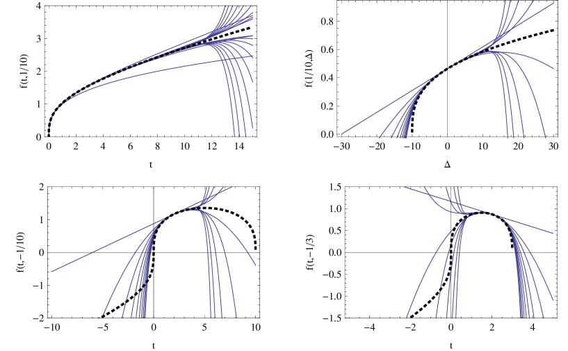
The efficacy of various expansions are illustrated in figure 19. In all the plots the black dotted line indicates the exact function. The top left panel shows successively higher order series approximations in $\Delta$ as a function of $t$ for the specific case $\Delta=1/10$. The question here is whether the pole at a given time lies with a disk of radius $1/10$? The location of the pole is $\Delta=-1/t$ so the answer is “yes” when $t>10$. This pole interferes with the convergence of the series expansion for $\Delta=1/10$. The figure demonstrates the (future) time of validity is $t<10$.

The top right panel shows the series in $\Delta$ at a fixed $t=1/10$. The question here is how big a perturbation will converge at $t=1/10$? Since the location of the pole is $\Delta=-1/t$ the radius of convergence at the indicated time is $10$. Perturbations with $|\Delta|>10$ are not expected to converge and the figure shows that this is indeed the case.

The bottom left panel shows the series in $t$ expanded around $t_{i}=2$ for fixed $\Delta=1/10$. The poles are at $t=-10$ and $t=0$ in the complex $t$ plane. The expected radius of convergence is $\min(|2-0|,|2-(-10)|)=2$ or $t_{i}-2<t<t_{i}+2$. As seen in the plot, the series converges only in the expected range $(0,4)$

The bottom right panel shows the series in $t$ expanded around $t_{i}=2$ for $\Delta=-1/3$. The poles are at $t=3$ and $t=0$ in the complex $t$ plane. The expected radius of convergence is $\min(|2-0|,|2-3|)=1$ or $t_{i}-1<t<t_{i}+1$. As seen in the plot, the series converges only in the expected range $(1,3)$.

Appendix C Parametric Solution

The background model has scale factor $a_{0}$ and Hubble constant $H_{0}={\dot{a}}_{0}/a_{0}$. The model, perturbed in density and velocity, is parameterized by $\Delta$ and $\theta$ and has scale factor $b(t)$. For the choice of coordinate system given in the text the second order equation for $b$ is

$$\frac{{\ddot{b}}}{b}=-\frac{1}{2}\frac{H_{0}^{2}a_{0}^{3}(1+\Delta\cos\theta)}{b^{3}}$$ (62)

with the initial conditions that at $t=t_{0}$, $b(t_{0})=a_{0}$, ${\dot{b}}(t_{0})={\dot{a}}_{0}(1+\Delta\sin\theta)$. The scale factor $a_{0}$ and the velocity of the background ${\dot{a}}_{0}$ at the initial time $t_{0}$ are positive. The parametrization of ${\dot{b}}(t_{0})$ allows either positive or negative values where $\Delta$ is non-negative and $-\pi<\theta\leq\pi$. The quantity $(1+\Delta\cos\theta)$, proportional to total density, is non negative.

This equation once integrated is

$${\dot{b}}^{2}=H_{0}^{2}a_{0}^{3}\left[\frac{(1+\Delta\cos\theta)}{b}+\frac{(1+\Delta\sin\theta)^{2}-(1+\Delta\cos\theta)}{a_{0}}\right].$$ (63)

The combination

$$E(\Delta,\theta)=(1+\Delta\sin\theta)^{2}-(1+\Delta\cos\theta)$$ (64)

is proportional to the total energy and determines the fate of the system. If $E(\Delta,\theta)>0$, the model is open and if $E(\Delta,\theta)<0$, the model is closed and will re-collapse eventually. Four cases (positive and negative $E$, positive and negative ${\dot{b}}_{0}$) are shown in figure 5.

C.1 Initially Expanding Solutions

The expanding case with ${\dot{b}}_{0}>0$ for open models ($E>0$) has solution

$$b(\eta,\Delta,\theta) = \frac{a_{0}}{2}\frac{(1+\Delta\cos\theta)}{E(\Delta,\theta)}(\cosh\eta-1)$$ (65)

$$t(\eta,\Delta,\theta) = \frac{1}{2H_{0}}\frac{(1+\Delta\cos\theta)}{E(\Delta,\theta)^{3/2}}(\sinh\eta-\eta)+t_{bang}^{+}(\Delta,\theta)$$ (66)

and the singularity $b=0$ occurs at $\eta=0$. For closed models ($E<0$) the solution is

$$b(\eta,\Delta,\theta) = \frac{a_{0}}{2}\frac{(1+\Delta\cos\theta)}{|E(\Delta,\theta)|}(1-\cos\eta)$$ (67)

$$t(\eta,\Delta,\theta) = \frac{1}{2H_{0}}\frac{(1+\Delta\cos\theta)}{|E(\Delta,\theta)|^{3/2}}(\eta-\sin\eta)+t_{bang}^{+}(\Delta,\theta).$$ (68)

For closed models, the convention adopted sets $\eta=0$ at the singularity nearest in time to $t_{0}$. For both models, the time at $\eta=0$ is denoted $t_{bang}^{+}$. For closed models the time at $\eta=2\pi$ is denoted $t_{coll}^{+}$.

At the initial time the solutions (both open and closed) satisfy $b(t_{0})=a_{0}$, ${\dot{b}}(t_{0})={\dot{a}}_{0}(1+\Delta\sin\theta)$ and $t=t_{0}$. The condition $b(t_{0})=a_{0}$ sets the value of the parameter at the initial time $\eta_{0}$. The velocity condition is then manifestly satisfied from the form of eq. (63). The condition $t=t_{0}$ at $\eta=\eta_{0}$ sets the value of the bang time

$$t_{bang}^{+}=t_{0}-\left\{\begin{array}[]{cc}\frac{1}{2H_{0}}\frac{(1+\Delta\cos\theta)}{|E(\Delta,\theta)|^{3/2}}(\eta_{0}-\sin\eta_{0})&E<0\\ \frac{1}{2H_{0}}\frac{(1+\Delta\cos\theta)}{E(\Delta,\theta)^{3/2}}(\sinh\eta_{0}-\eta_{0})&E>0.\end{array}\right.$$ (69)

The bang time for the model can also be written as

$$t_{bang}^{+}=t_{0}-\int_{b=0}^{b=a_{0}}\frac{db}{({\dot{b}}^{2})^{(1/2)}},$$ (70)

where ${\dot{b}}^{2}$ is given by eq. (63) with the sign for the square root positive. The age of the model since its birth is

$$t_{age}(\Delta,\theta)=\int_{b=0}^{b=a_{0}}\frac{db}{({\dot{b}}^{2})^{(1/2)}}=\int_{\eta=0}^{\eta=\eta_{0}}\frac{db/d\eta\cdot d\eta}{({\dot{b}}^{2}(\eta))^{(1/2)}}.$$ (71)

Inserting the appropriate parametric solution, one can verify that the bang times obtained from (69) and (70) are identical. Generally $t_{bang}^{+}\neq 0$.

The velocity at the initial time is

$${\dot{b}}_{0}={\dot{a}}_{0}|E|^{1/2}\left\{\begin{array}[]{cc}\frac{\sin\eta_{0}}{1-\cos\eta_{0}}&E<0\\ \frac{\sinh\eta_{0}}{\cosh\eta_{0}-1}&E>0.\end{array}\right.$$ (72)

First, ${\dot{b}}_{0}>0$ implies $\eta_{0}>0$. Second, if the age of the model increases, $\eta$ increases. For the open solution if $\eta$ varies from $0$ to $\infty$ time increases from $t_{bang}^{+}$ to $\infty$. For a single cycle of the closed solutions, $\eta$ increases from $0$ to $2\pi$ and time increases from $t_{bang}^{+}$ to $t_{coll}^{+}$.

In summary, the parametric solutions solve eq. (62) and eq. (63) for the specified initial conditions. As a final useful step, rewrite eq. (70) by defining $y=b/a_{0}$

$$t_{bang}^{+}=t_{0}-\frac{1}{H_{0}}\int_{y=0}^{y=1}\frac{dy}{\left[(1+\Delta\cos\theta)y^{-1}+E(\Delta,\theta)\right]^{1/2}}$$ (73)

which follows from eq. (63) and uses the same positive square root convention.

C.2 Initially Contracting Solutions

Next, consider the case ${\dot{b}}_{0}<0$. The parametric solution for $E>0$ is

$$b(\eta,\Delta,\theta) = \frac{a_{0}}{2}\frac{(1+\Delta\cos\theta)}{E(\Delta,\theta)}(\cosh\eta-1)$$ (74)

$$t(\eta,\Delta,\theta) = \frac{1}{2H_{0}}\frac{(1+\Delta\cos\theta)}{E(\Delta,\theta)^{3/2}}(-\sinh\eta+\eta)+t_{bang}^{-}(\Delta,\theta)$$ (75)

and for $E<0$ is

$$b(\eta,\Delta,\theta) = \frac{a_{0}}{2}\frac{(1+\Delta\cos\theta)}{|E(\Delta,\theta)|}(1-\cos\eta)$$ (76)

$$t(\eta,\Delta,\theta) = \frac{1}{2H_{0}}\frac{(1+\Delta\cos\theta)}{|E(\Delta,\theta)|^{3/2}}(-\eta+\sin\eta)+t_{bang}^{-}(\Delta,\theta).$$ (77)

Again, for closed models, the convention adopted is that the singularity nearest to $t_{0}$ corresponds to $\eta=0$. The time at $\eta=0$ is $t_{bang}^{-}$ and the collapse time for closed models is $t_{coll}^{-}$.

The parametric form of the solutions satisfies eq. (62) and eq. (63). Just as in the previous case, the initial conditions set $\eta_{0}$ and $t_{bang}^{-}$. Since the singularity at $\eta=0$ lies to the future of $t_{0}$,

$$t_{bang}^{-}=t_{0}+\int_{b=0}^{b=a_{0}}\frac{db}{(\dot{b}^{2})^{(1/2)}}.$$ (78)

where, ${\dot{b}}^{2}$ is given by eq. (63). The sign of the square root is chosen to be positive and the integral is a positive quantity which is added to $t_{0}$. For closed models the singularity at $\eta=2\pi$ lies to the past of $t_{0}$ at $t_{coll}^{-}$. In this case (see figure 5) the labelling implies $t_{coll}^{-}<t_{0}<t_{bang}^{-}$. Although this might seem backwards, it facilitates combining the open and closed models into one complex function as was done in the positive ${\dot{b}}_{0}$ case. The initial velocity is

$${\dot{b}}_{0}={\dot{a}}_{0}|E|^{1/2}\left\{\begin{array}[]{cc}\frac{\sinh\eta_{0}}{1-\cosh\eta_{0}}&E>0\\ \frac{\sin\eta_{0}}{\cos\eta_{0}-1}&E<0\end{array}\right.$$ (79)

The initial velocity ${\dot{b}}_{0}<0$ implies $\eta_{0}>0$. For the age of the model to increase, $\eta$ must decrease. Conversely, if $\eta$ increases, the time in the open model decreases from $t_{0}$ to $-\infty$ and the time in the closed model decreases from $t_{0}$ to $t_{coll}^{-}$.

A table summarising the properties of the physical solutions with $\bm{\eta}=|\bm{\eta}|\zeta=\eta\zeta$ follows.

	Closed	Open	If $\eta$ increases	If $t$ increases	$t_{bang}-t_{0}$
${\dot{b}}_{0}>0$	$\zeta=1$	$\zeta=i$	$t$ increases from $t_{bang}^{+}$	$\eta$ increases to $\infty$ or $2\pi$	$<0$
${\dot{b}}_{0}<0$	$\zeta=1$	$\zeta=i$	$t$ decreases from $t_{bang}^{-}$	$\eta$ decreases to $0$	$>0$

C.3 Analytic Extension of the exact solution in parametric form

The differential eq. (3.1) was solved numerically over the range $0\leq\theta\leq\pi$, $0<\delta<100$ and $-\pi<\phi\leq\pi$ where $\bm{\Delta}=\Delta e^{i\phi}$. For each value of $(\Delta,\phi,\theta)$, the numerical solution matched one of the two possible parametric forms.

Omitting the explicit functional dependence on $\bm{\Delta}$ and $\theta$ the following abbreviations are useful

$${\bf j} = (1+\bm{\Delta}\cos\theta)$$ (80)

$${\bf h} = \frac{(1+\bm{\Delta}\sin\theta)^{2}}{\bf j}$$ (81)

$${\bf E} = ({\bf h}-1){\bf j}.$$ (82)

The two possible parametric forms that agree with the numerical solution are

$${\bf b}(\eta) = \frac{a_{0}}{2}\frac{{\bf j}}{\left[-{\bf E}\right]}(1-\cos\eta)$$ (83)

$${\bf t}(\eta) = t_{0}\pm\left(\frac{1}{2H_{0}}\frac{\bf j}{\left[-{\bf E}\right]^{3/2}}(\eta-\sin\eta)-{\bf t_{age}}\right)$$ (84)

where

$${\bf t_{age}}=\frac{1}{H_{0}}\left(\sqrt{{\bf j}}\sqrt{{\bf h}}-\frac{{\bf j}}{\left[{\bf E}\right]^{3/2}}\sinh^{-1}\sqrt{\frac{\bf E}{\bf j}}\right).$$ (85)

The branch cut lies along the negative real axis for all fractional powers and from $-i\infty$ to $-i$ and $+i$ to $i\infty$ for the inverse sinh function.

The prescription for the correct form is for the choice of the $\pm$ sign in ${\bf t}$ eq. (84) and denoted ${\bf t}_{+}$ and ${\bf t}_{-}$. The correct form depends upon $\theta$, $\phi$, $\arg[{\bf h}]$ (the arg is defined to be between $-\pi$ and $\pi$) and the (real) value $j={\bf j}$ when $\phi=0$ or $\pi$. The figure 20 shows the upper half plane for the perturbation partitioned into areas where the complex extension of the solution has one of two forms. The lower half plane has the same structure inverted through the origin. The horizontal red dashed line denotes $\Delta\sin\theta=1$ and the vertical red dashed lines denote $\Delta\cos\theta=\pm 1$. In some areas a single form applies as marked but in the central area both occur. The detailed prescription is

$${\bf t}=\left\{\begin{array}[]{lr}0\leq\theta\leq\pi/4&\left\{\begin{array}[]{lr}\phi=\pi,|\Delta|\sin\theta<1\mbox{ and }j<0&{\bf t_{-}}\\ \\ \mbox{otherwise}&{\bf t}_{+}\\ \\ \end{array}\right.\\ \\ \pi/4<\theta\leq\pi&\left\{\begin{array}[]{lr}0<\phi<\pi\mbox{ and }\arg{\bf h}>0&{\bf t}_{+}\\ \\ -\pi<\phi<0\mbox{ and }\arg{\bf h}<0&{\bf t}_{+}\\ \\ \phi=0\mbox{ and }\left\{\begin{array}[]{c}\cos\theta>0\\ \mbox{ or}\\ \cos\theta<0\mbox{ and }j>0\end{array}\right.&{\bf t}_{+}\\ \\ \phi=\pi\mbox{ and }\left\{\begin{array}[]{c}\cos\theta<0\\ \mbox{ or}\\ \cos\theta>0\mbox{ and }j<0\end{array}\right.&{\bf t}_{-}\\ \\ \mbox{otherwise}&{\bf t}_{-}\end{array}\right.\\ \\ \end{array}\right.$$ (86)

Figure 20: This figure describes one aspect of the analytic extension of the exact solution. For a given real $\Delta$, the complex extension $\Delta\rightarrow\Delta e^{i\phi}$ obeys eq. (86) with two possible forms ${\bf t}_{+}$ and ${\bf t}_{-}$. The choice depends on $\phi$, $\Delta$, $\theta$. For some ($\Delta$, $\theta$) a single form is sufficient for all $\phi$; for other values both forms are needed. This figure illustrates how the upper half plane is partitioned based on this property. Coloured version online.

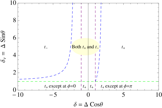
Appendix D Numerical solutions

D.1 Algorithm

The initial conditions are parameterized by $\Delta>0$ and $-\pi<\theta\leq\pi$. The transformation $\theta\rightarrow\pi\pm\theta$ and $\Delta\rightarrow-\Delta$ leaves the solution unchanged. At any time the roots for $\theta$ and $\pi\pm\theta$ are negatives of each other. The root plot only depends upon the absolute value of the root so the plots for $\theta$ and $\pi\pm\theta$ are identical. It is sufficient to consider the upper half plane.

For a given $\theta$ the algorithm to map out $R_{\Delta}(t)$ is the following: Vary $\Delta$ from $0$ to an arbitrarily large value ($\sim 100$) in small increments. For each $\Delta$ select $\bm{\Delta}=\Delta e^{i\phi}$ by varying the phase angles $\phi$ over the range $0$ to $2\pi$. For each $\bm{\Delta}$ evaluate ${\bf t}(\eta)$ at $\eta=0$ and $\eta=2\pi$ calculated according to eq. (86). Finally, hunt for solutions that set the imaginary part of ${\bf t}$ to $0$. This last step involves one-dimensional root-finding in $\phi$ at fixed $\Delta$. A solution leads to a specific pair $(t,\bm{\Delta})$ that is a pole in the function ${\bf b}(\bm{\Delta},t)$.

Roots with $t>t_{0}$ limit future evolution; those with $t<t_{0}$ limit backwards evolution. Both sets are shown in the results. Roots are classified based on whether they are real or complex. For closed models the real roots can represent a singularity that is nearby ($\eta=0$) or far away ($\eta=2\pi$) from $t_{0}$. This classification at the initial time is independent of whether the singularity is in the past or future and is independent of whether the model is expanding or contracting. For open models the real roots are always considered nearby ($\eta=0$).

In what follows the numerical answers are first described in qualitative terms. In the next section simple analytic estimates for the time of validity are developed.

Figure 21 shows the root plots on a log-log scale. Sixteen panels, each with a particular value of $\theta$ listed at the top, are displayed. The x-axis is $\log_{10}H_{0}t$ and the y-axis is the log of the distance of the singularity from the origin in the complex $\bm{\Delta}$ plane. The initial time, $H_{0}t_{0}=2/3$, is marked by the vertical black dashed line.

For each $\theta$, the shaded region indicates the range of $\Delta$ that gives rise to closed models. Figure 2 shows that closed models occur only for $\theta<\theta_{c}^{+}=0.463$ in the upper half plane so only some of the root plots have shading and then only at smaller $\Delta$.

The colour coding of the dots indicates four types of roots: real and complex roots where $\eta=2\pi$ are in blue and red, respectively; real and complex roots with $\eta=0$ are in cyan and pink, respectively. The radius of convergence at the initial time $t_{0}$ is infinite, i.e. the Lagrangian series is exact at the initial time by construction. At times very close to the initial time the root loci lie off the plot. Only the roots to the right of $H_{0}t_{0}$ are relevant for forward evolution and, conversely, only those to the left are relevant for backwards evolution. The discussion is focused on the case of forward evolution but it is straightforward to consider the restrictions on marching backwards in time.

The phase of the root (of smallest magnitude) appears in figure 23. When closed models have real roots they are positive; when open models have real roots they are negative. However, some open and closed models also possess complex roots. The set of models with complex roots (of smallest magnitude) is evident from the shading in figure 10. The phase of each root of smallest magnitude in figure 21 is indicated by the colour shading in figure 23.

There are horizontal dashed lines with colours green, blue and purple in figures 21 and 23 indicating $|\delta_{v}|=1$, $|\delta|=1$ and the transition between one and two complex forms, respectively. For each $\theta$ the lines mark the implied, special value of $\Delta$. These dashed lines also appear with the same colour coding in figure 22.

Figure 21: Root plots for $\theta$ in the range $0\leq\theta\leq\pi$. In each plot the abscissa is $\log_{10}H_{0}t$ and the ordinate is the logarithm of the magnitude of the root. The vertical black dashed line marks the initial time. The shaded area corresponds to closed models. The blue and red points show real and complex roots with $\eta=2\pi$, respectively. The cyan and pink show real and complex roots with $\eta=0$, respectively. The green and purple dashed lines are $|\delta_{v}|=1$ ($\Delta=|\sin\theta|^{-1}$) and $|\delta|=1$ ($\Delta=|\cos\theta|^{-1}$), respectively. The blue dashed line indicates the switch between two forms and a single form of the parametric solution at $\Delta=|2\sec\theta-\csc\theta|$. Coloured version online.

Figure 22: Several conditions determine the nature of the roots in phase space. The most significant are schematically illustrated here. The green horizontal lines are $|\delta_{v}|=\Delta|\sin\theta|=1$; purple vertical lines are $|\delta|=\Delta|\cos\theta|=1$; the black curved line is the $E=0$ critical solution. The red lines $\Delta_{rc}$ mark where real roots associated with closed models (or closed mirror models) transform to complex roots. The blue dashed lines mark the division between one and two complex forms (see also figure 20). Physical models lie to the right of $\delta=-1$. Expanding models lie above $\delta_{v}=-1$. The intersection $\delta=\delta_{v}=1$ occurs at $\theta=\pi/4$. The point P near $\theta=0.84$ is the meeting of $\delta_{v}=1$ and $\Delta_{rc}$. Coloured version online.

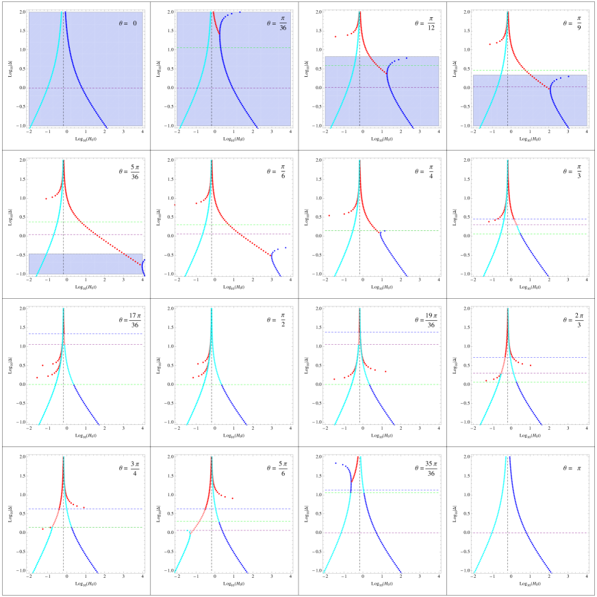
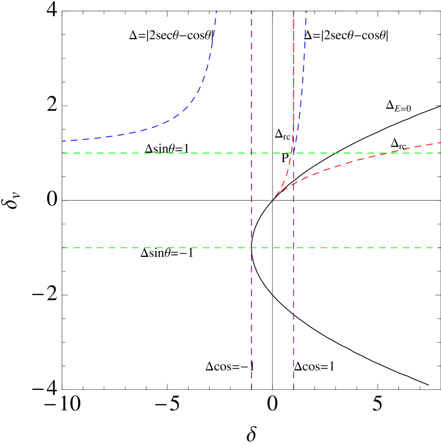
The roots in figure 21 will be analysed in the range $0<\theta\leq\pi/4$, $\pi/4<\theta\leq\pi/2$, $\pi/2<\theta\leq\pi$.

D.1.1 $0\leq\theta\leq\pi/4$

The top left panel in figure 21 has $\theta=0$; the blue dots indicate real roots with $\eta=2\pi$; the blue shading indicates a closed model; the phase is positive (top left panel in figure 23). Only a single branch is evident. In sum, each root is the collapse time of a closed, pure density perturbation. For an expanding model, $\eta=2\pi$ implies that the root is the future singularity. That $\theta=0$ is a special case can be seen by consulting figure 22: a ray starting at $\Delta=0$ with $\theta=0$ never intersects any of the other lines of the diagram. In general, each time a ray crosses one of the lines there is qualitative change in the properties of the roots.

For $0<\theta\leq\pi/4$ a great deal more complexity is evident in figure 21. First, consider a ray emanating with small angle $0<\theta<\theta_{c}^{+}$ in figure 22 ($\tan\theta_{c}^{+}=1/2$ is the slope of the $E=0$ line at the origin). Eventually such a line will cross the black line which is the $E=0$ critical solution labelled $\Delta_{E=0}$. For small $\Delta$ the models are closed; for larger $\Delta$ they are open. In figure 21 this distinction corresponds to the the blue shading (closed models) at small $\Delta$ versus the unshaded (open) models at large $\Delta$.

Within the shaded region note that two branches of real roots are present beyond a given time; at large $t$ (asymptotically) the lower branch is $\Delta\to 0$ and the upper branch is $\Delta\to\Delta_{E=0}$. The lower branch sets the time of validity for small $\Delta$. Each root is the collapse time of a closed model which has both density and velocity perturbations at the initial time.

As $\Delta$ increases the time of validity inferred from the lower branch decreases. At the critical point $\Delta=\Delta_{rc}$, the two real branches merge and connect to a branch of complex roots (intersection of red and blue points). For $\Delta>\Delta_{rc}$, the complex roots determine the time of validity even though the upper branch provides a real root. The complex roots do not have a direct physical interpretation in terms of future singularities of physical models. On figure 22 the ray emanating from the origin at shallow angle crosses the red dashed line labelled $\Delta_{rc}$ at this critical point.

Physically, when $\Delta$ exceeds $\Delta_{rc}$, the velocity perturbation dominates the density perturbation in the sense that the collapse time begins to increase. The real root corresponds to the future singularity of the model. As $\Delta$ increases further, the solution eventually becomes critical (infinite collapse time). The particular value where this occurs is $\Delta_{E=0}$ and it corresponds on figure 22 to the ray crossing the labelled black line. Within the entire range $\Delta_{rc}<\Delta<\Delta_{E=0}$ the complex root determines the time of validity. So, even though any model in this range is closed and possesses a real future singularity, the time of validity is determined by the complex root. This gives the sliver on figure 10 which is the overlap of light red and blue shadings.

Both $\Delta_{rc}$ and $\Delta_{E=0}$ decrease as $\theta\to\theta_{c}^{+}$ as is evident from figure 22 and both vanish at $\theta_{c}^{+}$. On figure 21 the real roots completely disappear and only the complex roots are present, i.e. the two real branches have been pushed out to infinite times. The panel with $\theta=5\pi/36=0.436$ is numerically closest to the critical case $\theta_{c}^{+}=0.464$ and the real branches are just barely visible at the right hand edge.

For the rest of the upper half plane $\theta_{c}^{+}<\theta\leq\pi$ the ray no longer intersects any closed models.

For $\theta_{c}^{+}<\theta<\pi/4$ the real roots reappear and move back to the left in figure 21 (see panel with $\theta=\pi/6$). Now, however, the roots are negative (see figure 23). This is a manifestation of mirror symmetry which relates the negative real roots of an open model to the positive real roots of a closed model. At large $t$ the two branches have $\Delta\to 0$ and $\Delta\to\Delta_{E=0}$ and are completely analogous to the real branches just discussed for closed models. The separation between the two real branches increases as $\theta$ increases and the solution loci shifts upwards in $\Delta$. And just as before the two branches join and meet a complex branch. The second red dashed line $\Delta_{rc}$ in figure 22 shows the real to complex transition for the roots for the open models.

This behaviour might be expect to continue for $\pi/4<\theta<\pi$ but there is an additional complication: the analytic extension involves two forms. As the ray sweeps counterclockwise in figure 20 it crosses $\delta_{v}=1$ (horizontal dashed line and the curved blue line. These are also schematically illustrated in figure 22.

D.1.2 $\pi/4<\theta<\pi/2$

All physical models are in this range are open. Real roots have a straightforward interpretation in terms of the mirror models. Although some of the analysis described for $\theta<\pi/4$ continues to apply several additional complications ensue. To understand them it is useful refer to the phase space picture shown in figure 22. As $\theta$ increases, the point where $\Delta_{rc}$ meets $\delta_{v}=1$ is labelled P.

For a fixed $\theta$ consider increasing $\Delta$ from small values near the origin to $\infty$. The order in which this ray intersects the green ($\delta_{v}=1$), purple ($\delta=1$), red ($\Delta_{rc}$) and blue (one or two complex forms) curves will correlate with the change in roots.

The roots are negative real for small $\Delta$. They correspond to the collapse time of a closed mirror model. Increase $\Delta$ and ignore $\Delta_{rc}$. When the $\delta_{v}=1$ line is crossed, the sign of the closed mirror model’s velocity switches from expanding to contracting. This just means that the labelling of the future singularity switches from further away ($\eta=2\pi$) to nearer ($\eta=0$). Now recall $\Delta<\Delta_{rc}$ implies real roots and, by definition, $\delta_{v}=\Delta\sin\theta$. Hence, $\Delta_{rc}(\theta)>1/\sin\theta$ implies that the label switch occurs just as outlined. On figure 22 rays counterclockwise of point P belong to this case. This is responsible for the switch from blue (real $\eta=2\pi$) to cyan (real $\eta=0$) roots at the green line in figure 21 for $\theta=\pi/3$ and $17\pi/36$.

Conversely, if $\Delta_{rc}(\theta)<1/\sin\theta$ the roots are already complex and the label switch occurs between the corresponding complex roots. There are no pictured examples in figure 21.

In the previous section with the $0<\theta\leq\pi/4$, the physical interpretation of $\Delta_{rc}$ (as $\Delta$ increases) was that the velocity contribution to the perturbation became dominant in the original model if the model was closed or in the mirror closed model if the original model was open. In latter case the mirror models were initially expanding. Now, the same idea continues to apply in the regime $\pi/4<\theta<0.84$. Here the transition from real to complex roots occurs before the $\delta_{v}=1$ line is crossed. The significance of $\Delta_{rc}$ is that it marks the increasing importance of velocity perturbations in the closed expanding mirror models.

However, for $0.84<\theta<\pi/2$ as $\Delta$ increases the open model crosses $\delta_{v}=1$, the mirror model swaps from $\eta=2\pi$ to $0$ and the roots (real) corresponds to the real future singularity of a closed, contracting model. As $\Delta$ increases further, first the mirror model becomes critical and then an open model contracting to a future singularity. While the magnitude of $\Delta$ grows larger than a critical value the velocity perturbation dominates the mirror model dynamics. When $\Delta>\Delta_{rc}$ the roots switch from real to complex. At this point the contracting mirror model can be open, closed or critical.

Note in figure 22 that $\Delta_{rc}$ asymptotes to the vertical purple line $\delta=1$. The corresponding mirror model hits the line $\delta=-1$ in the third quadrant. This is the limiting vacuum solution. Although there are no physical models beyond the analytic extension continues and the roots change from real to complex. All open models with $\theta\mathbin{\lower 3.0pt\hbox{$\hbox to0.0pt{\raise 5.0pt\hbox{$\char 60\relax$}\hss}\mathchar 29208\relax$}}\pi/2$ see a transition to complex roots as the mirror approaches the vacuum solution.

Finally figure 22 shows as a blue curve the point at which there is a switch in complex form of the analytic extension. Here, the complex roots switch from $\eta=0$ to $\eta=2\pi$. The roots remain complex and since there is no physical interpretation and it is irrelevant whether they belong to $\eta=0$ or $\eta=2\pi$.

In figure 21 the panel with $\theta=\pi/3$ and $17\pi/36$ show these transitions: the blue to cyan transition at the green dashed line is the mirror model switch from expanding to contracting; the cyan to pink transition at the purple dashed line is the mirror model moving through $\delta=-1$; the pink to red transition is the switch from two to one complex roots and $\eta=0$ to $\eta=2\pi$.

D.1.3 $\theta=\pi/2$

At $\theta=\pi/2$, only real roots of $\eta=0$ are present for large $\Delta$. This is a special case in that a ray only intersects one special line $\delta_{v}=1$ in the upper half plane.

D.1.4 $\pi/2<\theta\leq\pi$

All models in this range also correspond to open models. Like the previous cases, small $\Delta$ have real, negative roots with $\eta=2\pi$. The mirror models in this case lie in the fourth quadrant. The crossover of real roots from $\eta=0$ to $\eta=2\pi$ occurs at $\delta_{v}=1$, however, unlike in the earlier case, the line $\delta=-1$ is never approached by the mirror models in the fourth quadrant. As a result, there is no switch from real to complex roots and all models have real negative roots. The $\eta=2\pi$ roots for small $\Delta$ are collapse times of initially expanding closed mirror models and the $\eta=0$ are future singularities of initially contracting closed and open mirror models for intermediate and large values of $\Delta$ respectively.

Figure 23: Roots with $\eta=2\pi$ plotted in the complex $\Delta$ plane for $0<\theta\leq\pi$. These values of $\theta$ correspond to those in figure 21. The colour codes the complex phase of the roots ($\bm{\Delta}=\Delta e^{i\phi}$). The real positive ($\phi=0$) and negative ($\phi=\pi$) roots are shown in red and cyan respectively. The complex roots can have any colour other than these two and the bottom figure provides the coding. By comparison with figure 21 one sees that all open models with real roots are cyan (negative); likewise all closed models with real roots are red (positive). Note, however, that there exist complex roots for both open and closed models. Coloured version online.

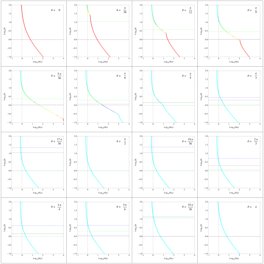
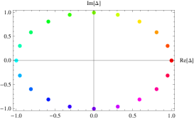
D.2 Numerical Results

Here we present numerical formulas that give the time of validity for any initial $\Delta$ and $\theta$. Real roots occur for small $\Delta$ when $0<\theta<\pi/2$; and they occur for all $\Delta$ when $\pi/2\leq\theta\leq\pi$ or $\theta=0$. Real roots correspond to past or future singularities of physical models and are known exactly.

Figure 21 shows that complex roots occur $0<\theta<\pi/2$. In the range $\pi/4<\theta<\pi/2$ figure 23 shows that the phase of the complex roots is very close to $\pi$. We can approximate these roots as real, negative roots. Conversely, figure 23 also shows that in the range $0<\theta\leq\pi/4$ the phase is not close to $0$ or $\pi$. These roots are complex only when $\Delta>\Delta_{rc}$. First, we fit $\Delta_{rc}$ by

$$\Delta_{rc,app}(\theta)=\left|0.41\csc^{2}\theta(\cos\theta-2\sin\theta)+3.57(\cos\theta-2\sin\theta)(\sin\theta)^{4.39}\right|.$$ (87)

We cannot approximate the time of validity with the results for physical cases but it turns out that the numerically derived time of validity is insensitive to $\theta$ in the range $0<\theta<\pi/4$ and may be fit

$$H_{0}t_{app}(\Delta)=\frac{2}{3}+\left\{\begin{array}[]{cc}\frac{14.125}{\Delta^{2.5}}&0<\Delta\leq 1\\ \frac{1.514}{\Delta^{2.82}}&1<\Delta\leq 2\\ \frac{1.778}{\Delta^{3.13}}&2<\Delta\leq 5\\ \frac{63095}{\Delta^{9.6}}&5<\Delta\leq 10\\ \frac{2\times 10^{6}}{\Delta^{8.5}}&\Delta>10.\end{array}\right.$$ (88)

Using these quantities, the table below gives an approximation to the time of validity, $T_{app}$, for all values of $\theta$ and $\Delta$. The times for collapse and the bang times are equivalent to eq. (84) and reproduced here for convenience:

$$t_{coll}(\Delta,\theta) = t_{0}+\frac{1}{2H_{0}}\frac{(1+\Delta\cos\theta)}{\left[-E(\Delta,\theta)\right]^{3/2}}(2\pi)-t_{age}(\Delta,\theta)$$ (89)

$$t_{bang}^{-}(\Delta,\theta) = t_{0}+t_{age}(\Delta,\theta)$$ (90)

where,

$$t_{age}(\Delta,\theta) = \frac{1}{H_{0}}\sqrt{(1+\Delta\cos\theta)}\sqrt{\frac{(1+\Delta\sin\theta)^{2}}{(1+\Delta\cos\theta)}}-\frac{1}{H_{0}}\frac{(1+\Delta\cos\theta)}{\left[E(\Delta,\theta)\right]^{3/2}}\sinh^{-1}\sqrt{\frac{E(\Delta,\theta)}{(1+\Delta\cos\theta)}},$$ (91)

$$E(\Delta,\phi,\theta) = (1+\Delta\sin\theta)^{2}-(1+\Delta\cos\theta)$$ (92)

Table 1: Approximation to time of validity, $T_{app}(\Delta,\theta)$, for $0\leq\theta\leq\pi$. Note that $\Delta_{rc,app}$ is an approximation to $\Delta_{rc}$ in eq. (87).

Parameter range			$T_{app}$
	$0<\Delta<\Delta_{rc,app}$	$E(\Delta,\theta)<0$	$t_{coll}(\Delta,\theta)$
$0<\theta<\pi/4$	$0<\Delta<\Delta_{rc,app}$	$E(\Delta,\theta)>0$	$t_{coll}(-\Delta,\theta)$
	$\Delta>\Delta_{rc,app}$		$t_{app}(\Delta,\theta)$
	$0<\Delta<\frac{1}{|\sin\theta|}$		$t_{coll}(-\Delta,\theta)$
$\pi/4<\theta\leq\pi/2$	$\frac{1}{|\sin\theta|}\leq\Delta\leq\left|\frac{2\sin\theta-\cos\theta}{\sin\theta\cos\theta}\right|$		$\Re\left[t_{bang}^{-}(-\Delta,\theta)\right]$
	$\Delta>\left|\frac{2\sin\theta-\cos\theta}{\sin\theta\cos\theta}\right|$		$\Re\left[t_{coll}(-\Delta,\theta)\right]$
	$0<\Delta\leq\frac{1}{|\sin\theta|}$		$t_{coll}(-\Delta,\theta)$
$\pi/2\leq\theta\leq\pi$	$\Delta>\frac{1}{|\sin\theta|}$		$t_{bang}^{-}(-\Delta,\theta)$

The error in the fit is estimated as

$${\cal E}=\frac{T-T_{app}}{T}.$$ (93)

If ${\cal E}>0$ then the approximation is conservative in this sense: the approximate time of validity is less than the true value. Conversely, if ${\cal E}<0$, then the approximation overestimates the time of validity. Using the above fits the worst case is ${\cal E}\simeq-0.02$. We always use a time step $\delta t$ which satisfies $\delta t<0.98T_{app}$ so that the inaccuracy in the approximation is irrelevant.

Appendix E Error characterisation of the Lagrangian series

We want to characterise the errors associated with calculating the solution at time $t_{f}$ given some fixed initial conditions at time $t_{0}$. Errors arise because any real calculation involves truncating the Lagrangian expansion. We want to compare the errors that result from different choices of truncation order and of the number of re-expansion steps assuming all series expansions are convergent (i.e. all respect the time of validity). Let $N_{m}$ represent the final physical coordinate generated with a $m$-th order calculation using $N$ steps. Ultimately, we seek to characterise differences like $N_{m}-{N^{\prime}}_{m^{\prime}}$. The quantity $1_{\infty}$ is the exact answer.

E.0.1 Single step

The Lagrangian series solution for a single step has the form

$$1_{\infty}=a(t)\left(1+\sum_{i=1}^{\infty}\frac{b^{(i)}(t)}{a(t)}\Delta_{0}^{i}\right)X_{0},$$ (94)

where each $b^{(i)}$ satisfies

$${\ddot{b}}^{(i)}-\frac{H_{0}^{2}a_{0}^{3}b^{(i)}}{a^{3}}=S^{(i)}$$ (95)

and initial conditions are specified at $t=t_{0}$. The initial conditions at each order and the forms for the first few $S^{(i)}$ are given in the text.

If $t_{f}-t_{0}=\delta t<<t_{0}$, then the solutions can be expanded in the small parameter $\delta t/t_{0}$. The solutions are

$$b^{(1)}(t)/a(t) \sim c^{(1)}\frac{\delta t}{t_{0}},$$ (96)

$$b^{(i)}(t)/a(t) \sim c^{(i)}\left(\frac{\delta t}{t_{0}}\right)^{i+1}\mbox{ for }i\geq 2.$$ (97)

The coefficients $c^{(i)}$ depend on the angle $\theta$ and have a weak dependence on the Lagrangian order. The difference between the exact answer and the $m$-th order approximation for a single step is

$$1_{\infty}-1_{m}=\left(\sum_{i=m+1}^{\infty}c^{(i)}\left(\frac{\delta t}{t_{0}}\right)^{i+1}\Delta_{0}^{i}\right)X_{0}.$$ (98)

As long as $t_{f}$ is within the time of validity of LPT, by definition, the LPT series converges and from the equation above, the leading order error scales as $\sim(\delta t/t_{0})^{m+2}\Delta^{m+1}$ (order terms first by powers of $\Delta$ and then by powers of $\delta t/t_{0}$).

E.0.2 Multiple steps

In general for a practical application one is limited to working at a finite Lagrangian order. In such cases, it becomes necessary to ask if convergence can be achieved by working at a finite Lagrangian order with increasing number of steps.

First, we outline the calculation. The initial data is subscripted by “0”. For example, let the initial perturbed scale factor be $b_{0}=b(t_{0})$, the initial background scale factor $a_{0}$, the initial density contrast $\delta_{0}$ and the initial velocity perturbation $\delta_{v0}$. The Lagrangian expansion parameter $\Delta_{0}$ and angle $\theta_{0}$ follow from the relations $\delta_{0}=\Delta_{0}\cos\theta_{0}$ and $\delta_{v0}=\Delta_{0}\sin\theta_{0}$. The physical coordinate is $r_{0}=b_{0}X_{0}$; for given $r_{0}$ the initial Lagrangian coordinate $X_{0}$ is fixed by choosing $b_{0}$ to be equal to $a_{0}$.

Consider taking $N$ steps from initial to final time with an $m$-th order Lagrangian expansion. Assume that the final time is within the time of validity of the Lagrangian expansion. For definiteness, let the $j$-th time be $t_{j}=t_{0}\beta^{j/N}$ where $\beta=t_{f}/t_{0}$ (so $t_{N}$ is just the final time $t_{f}$). This geometric sequence of increasing steps is well-suited for an expanding background with a small growing perturbation. The scaling of differences like $N_{m}-1_{\infty}$, $(N+1)_{m}-N_{m}$ and $N_{m+1}-N_{m}$ with $N$ and $m$ are all of interest. We expect the same scaling of these differences with $N$ and $m$ for any uniformly refined set of time steps.

A finite order Lagrangian expansion accurate to order $m$ is a truncated representation of the full Lagrangian solution

$$b(t)=\sum_{i=0}^{m}b^{(i)}(t)\Delta_{0}^{i}.$$ (99)

At the beginning of the first step the scale factor at $t_{0}$ is advanced to $t_{1}$ and written as $b(t_{0}\to t_{1};\Delta_{0},\theta_{0})$. Note the explicit dependence on the perturbation parameters at $t_{0}$. Abbreviate the scale factor and its derivative for the truncated expression as $b$ and ${\dot{b}}$. The background scale factor at time $t_{1}$ is $a_{1}$. At the end of the first step the Lagrangian coordinate $X_{1}$ and the new $b_{1}$ are inferred as described in the main body of the text by re-scaling quantities calculated at $t_{1}$. The new $b_{1}$ is not $b$. The net result for the full step $t_{0}\to t_{1}$ is

$$X_{1} = X_{0}\frac{b}{a_{1}}$$ (100)

$$b_{1} = a_{1}$$ (101)

$${\dot{b}}_{1} = \frac{{\dot{b}}}{b}a_{1}$$ (102)

$$\delta_{1} = (1+\delta_{0})\left(\frac{a_{1}}{b}\right)^{3}-1$$ (103)

$$\delta_{v1} = \frac{a_{1}{\dot{b}}}{{\dot{a}}_{1}b}-1.$$ (104)

The newly defined quantities subscripted by “1” will be used to initiate the next step. The updated perturbations imply new Lagrangian expansion parameter and angle according to

$$\Delta_{1} = \sqrt{\delta_{1}^{2}+\delta_{v1}^{2}}$$ (105)

$$\cos\theta_{1} = \frac{\delta_{1}}{\Delta_{1}}$$ (106)

$$\sin\theta_{1} = \frac{\delta_{v1}}{\Delta_{1}}.$$ (107)

The new physical position is $r_{1}=b_{1}X_{1}=bX_{0}$. In a numerical calculation the truncated $b$ is exact to floating point precision but contains an error because of the omitted orders; in a symbolic calculation $b$ is known to order $\Delta_{0}^{m}$.

The next step from $t_{1}\to t_{2}$ involves a similar update with $b=b(t_{1}\to t_{2};\Delta_{1},\theta_{1})$

$$X_{2} = X_{1}\frac{b}{a_{2}}$$ (108)

$$b_{2} = a_{2}$$ (109)

$${\dot{b}}_{2} = \frac{{\dot{b}}}{b}a_{2}$$ (110)

$$\delta_{2} = (1+\delta_{1})\left(\frac{a_{2}}{b}\right)^{3}-1$$ (111)

$$\delta_{v2} = \frac{a_{2}{\dot{b}}}{{\dot{a}}_{2}b}-1.$$ (112)

The new physical position is $r_{2}=b_{2}X_{2}$. This iterative scheme repeats for a total of $N$ steps. It ultimately yields an approximation to the position at the final time denoted $N_{m}=b_{N}X_{N}$.

A difference like $(N+1)_{m}-N_{m}$ may be calculated numerically for various $N$ and $m$ and the scaling fitted and inferred. In addition, one can approach the problem symbolically. To write $N_{m}$ we need to expand the final result in powers of $\Delta_{0}$. Note, for example, that $\Delta_{1}$ and $\theta_{1}$ are known as expansions in $\Delta_{0}$ with coefficients that depend upon $\theta_{0}$. Perturbation-related quantities are re-written systematically in terms of initial quantities. For example, $b(t_{1}\to t_{2};\Delta_{1},\theta_{1})$ may be expanded in powers of $\Delta_{1}$ with coefficients depending upon $\theta_{1}$. Next, all occurrences of $\Delta_{1}$ and $\theta_{1}$ are replaced by expansions in powers of $\Delta_{0}$ and coefficients depending upon $\theta_{0}$. All terms up to and including $\Delta_{0}^{m}$ are retained in the final result. This procedure is systematically repeated until all quantities are expressed in terms of initial data. Finally, the difference $(N+1)_{m}-N_{m}$ is calculated symbolically. Similar strategies allow construction of all the differences of interest.

To make analytic progress assume that $f_{t}=\beta-1=(t_{f}-t_{0})/t_{0}<<1$ is a small parameter. In a difference like $(N+1)_{m}-N_{m}$ many “lower order” terms will coincide. Consider an ordering of terms by the powers of $\Delta_{0}$ (first) and by powers of $f_{t}$ (second). Define the leading-order difference to be the first non-vanishing term proportional to $\Delta_{0}^{p}f_{t}^{q}$ for smallest $p$ and then smallest $q$. It is straightforward to apply this ordering to simplify the differences like $(N+1)_{m}-N_{m}$. The leading order differences satisfy the following simple equalities

$$|1_{\infty}-N_{m}| \sim |g_{N,m}|$$

$$|N_{m+1}-N_{m}| \sim |g_{N,m}|$$ (113)

$$|(N+1)_{m}-N_{m}| \sim |g_{N+1,m}-g_{N,m}|$$

where

$$g_{N,m} = K_{N,m}\cos\theta\sin^{m}\theta\Delta^{m+1}f_{t}^{m+2}$$

$$K_{N,m} = \frac{1}{9}\left(\frac{-2}{3}\right)^{m}\left(\frac{N-\frac{m}{2+m}}{N^{m+1}}\right).$$

These differences can be compared with the numerical differences for which no expansion in $f_{t}$ is carried out.

We verified the analytical scaling by the following numerical experiment. The parameters of the problem at the starting time $t_{0}$ are $\Delta_{0}=1/2$, $\theta_{0}=-\pi/4$. The final time of interest $t_{f}$ is close to the initial time so that $(t_{f}-t_{0})/t_{0}=1/4$. The $m$-th order Lagrangian approximation is evaluated at this fixed final time with successively increasing number of steps. Values of $m$ from 1 to 4 and values of $N$ from 10 to 50 were considered. For geometric time steps $(t_{i+1}-t_{i})/t_{i}=\beta^{1/N}-1$ is independent of $i$ and denoted $\delta t/t$ below.

The results are plotted in figure 24. The points indicate the numerical data points and the solid lines indicate the analytical functions defined in eq. (E.0.2). The numerical calculation was done with a high enough precision that even small errors of the order of $10^{-14}$ are not contaminated by floating point errors. The agreement between the numerical experiment and the symbolic differences is very good.

Figure 24: The three panels show the log of the errors $|1_{\infty}-N_{m}|$, $|N_{m+1}-N_{m}|$ and $|(N+1)_{m}-N_{m}|$ vs. $N$. The final time $t_{f}$ is the same for all these comparisons. The dots correspond to the data generated by the numerical experiment and lines correspond to the analytical formulas given in eq. (E.0.2). The lines from top to bottom correspond to $m=1,2,3,4$ respectively for the first and third panels and to $m=1,2,3$ for the second panel. It is clear that for a fixed $m$, increasing the number of steps improves convergence. Conversely, for a fixed $N$, increasing the Lagrangian order $m$ improves convergence.

Thus, the scaling of the errors implies that for a small total time step, any finite order Lagrangian scheme will yield convergent results upon taking multiple steps. Conversely, for a fixed number of steps, a higher order Lagrangian calculation will give better results.

It is useful to express the scaling in terms of the individual small step size $\delta t/t$. Under the assumptions that $(t_{f}-t_{0})/t_{0}$ is small, $(t_{f}-t_{0})/t_{0}\sim N\delta t/t$. The scaling $|1_{\infty}-N_{m}|\sim N^{-m}\Delta^{m+1}((t_{f}-t_{0})/t_{0})^{m+2}$ can be re-written as $|1_{\infty}-N_{m}|\sim N((t_{f}-t_{0})/t_{0})\cdot\Delta^{m+1}(\delta t/t)^{m+1}$, which can be interpreted as an error of $((t_{f}-t_{0})/t_{0})\Delta^{m+1}(\delta t/t)^{m+1}$ per step. In the text, the quantity $\epsilon=\Delta\delta t/t$ is kept constant. For fixed initial and final times, the error scales $\propto N\epsilon^{m+1}$. If $\Delta$ does not change appreciably then the error is $\propto\Delta\epsilon^{m}$. Convergence is attained when $\epsilon\to 0$.

References

- Adler & Buchert (1999) Adler S., Buchert T., 1999, A&A, 343, 317
- Bernardeau et al. (2002) Bernardeau F., Colombi S., Gaztañaga E., Scoccimarro R., 2002, Phys. Rep., 367, 1
- Bouchet (1996) Bouchet F. R., 1996, astro-ph/9603013
- Bouchet et al. (1995) Bouchet F. R., Colombi S., Hivon E., Juszkiewicz R., 1995, A&A, 296, 575
- Bouchet et al. (1992) Bouchet F. R., Juszkiewicz R., Colombi S., Pellat R., 1992, ApJ, 394, L5
- Brown & Churchill (1996) Brown J. W., Churchill R., 1996, Complex Variables and Applications. Weily
- Buchert (1992) Buchert T., 1992, MNRAS, 254, 729
- Buchert (1994) Buchert T., 1994, MNRAS, 267, 811
- Buchert (1995) Buchert T., 1995, astro-ph/9509005
- Buchert et al. (1999) Buchert T., Dominguez A., J.Perez-Mercader 1999, A&A, 349, 343
- Buchert & Ehlers (1993) Buchert T., Ehlers J., 1993, MNRAS, 264, 375
- Catelan (1995) Catelan P., 1995, MNRAS, 276, 115
- Chicone (2006) Chicone C., 2006, Ordinary Differential Equations with Applications, (section 1.1, 1.12), second edn. Texts in Applied Mathematics, New York: Springer-Verlag
- Ehlers & Buchert (1997) Ehlers J., Buchert T., 1997, General Relativity and Gravitation, 29, 733
- Karakatsanis et al. (1997) Karakatsanis G., Buchert T., Melott A., 1997, A&A, 326, 873
- Kasai (1995) Kasai M., 1995, Phys. Rev. D, 52, 5605
- Landau & Lifshitz (1975) Landau L. D., Lifshitz E. M., 1975, The Classical Theory of Fields, fourth edn. Butterworth Heinemann
- Matarrese et al. (1993) Matarrese S., Pantano O., Saez D., 1993, Phys. Rev. D, 47, 1311
- Matarrese et al. (1994) Matarrese S., Pantano O., Saez D., 1994, MNRAS, 271, 513
- Matarrese & Terranova (1996) Matarrese S., Terranova D., 1996, MNRAS, 283, 400
- Monaco (1997) Monaco P., 1997, MNRAS, 287, 753
- Moutarde et al. (1991) Moutarde F., Alimi J., Bouchet F. R., Pellat R., Ramani A., 1991, ApJ, 382, 377
- Munshi et al. (1994) Munshi D., Sahni V., Starobinsky A. A., 1994, ApJ, 436, 517
- Sahni & Coles (1995) Sahni V., Coles P., 1995, Phys. Rep., 262, 1
- Sahni & Shandarin (1996) Sahni V., Shandarin S., 1996, MNRAS, 282, 641
- Scoccimarro & Sheth (2002) Scoccimarro R., Sheth R. K., 2002, MNRAS, 329, 629
- Tatekawa (2007) Tatekawa T., 2007, Phys. Rev. D, 75, 44028
- Tolman (1934) Tolman R. C., 1934, Proceedings of the National Academy of Science, 20, 169
- Zel’Dovich (1970) Zel’Dovich Y. B., 1970, A&A, 5, 84