Quantum Monte Carlo for minimum energy structures
Abstract
We present an efficient method to find minimum energy structures using energy estimates from accurate quantum Monte Carlo calculations. This method involves a stochastic process formed from the stochastic energy estimates from Monte Carlo that can be averaged to find precise structural minima while using inexpensive calculations with moderate statistical uncertainty. We demonstrate the applicability of the algorithm by minimizing the energy of the H2O-OH- complex and showing that the structural minima from quantum Monte Carlo calculations affect the qualitative behavior of the potential energy surface substantially.
pacs:
PACS:02.50.Ey,02.70.Ss, 02.50.Fz, 02.60.PnFirst principles electronic structure methods have been used to describe and explain a wide range of properties for different condensed matter systems. A critical step is the accurate determination of the ground state atomic structure, since many important properties of a material can change dramatically depending on the structure. Because of the balance between accuracy and computational cost, density functional theory (DFT) has become a commonly used method to find equilibrium geometries of both molecules and extended systems. The primary reason for this is the availablility of forces with little extra computational cost over the energy calculation. Using a typical quasi-Newton minimization algorithm, the local minimum of a potential energy surface can be found in , where is the number of degrees of freedom to be optimized. This favorable scaling has made it possible to find minima for many systems of interest. However, in many situations, including transition metals, excited states, and weak binding, current density functional theories may not be accurate enough even for structures, and more accurate post-Hartree-Fock methods that scale as , where is the number of electrons, can often be too computationally expensive.
Quantum Monte Carlo (QMC), a stochastic approach to solving the many-body Schrödinger equation, offers favorable scaling to obtain the total energy, , and has been shown to provide near chemical accuracy in many different systemsKolorenč and Mitas (2008); Grossman (2002). However, there are two major challenges in using QMC methods to obtain high precision minimum energy structures. The first is that the techniques so far proposed to calculate forces in diffusion Monte Carlo all have large variances and error terms that depend on the quality of the trial wave function, which is often poor in systems where DFT fails and one would like to apply QMC methods. In fact, despite much work in recent yearsChiesa et al. (2005); Assaraf and Caffarel (2003); Casalegno et al. (2003); Badinski and Needs (2007); Badinski et al. (2008); Filippi and Umrigar (2000), QMC forces using the highly accurate diffusion Monte Carlo method have not been applied to more than a few degrees of freedom, although the simpler variational Monte Carlo technique has been applied to moreAttaccalite and Sorella (2008). The second challenge is the stochastic nature of Monte Carlo algorithms, which provides uncertainty in any estimator that only decreases as the square root of the computer time. Reducing the uncertainty enough to resolve the minimum structure accurately using forces or total energies is often prohibitively expensive computationally. Methods such as the stochastic gradient approximationRobbins and Monro (1951); Harju et al. (1997) that are able to operate in the presence of noise suffer from this large uncertainty in the forces. As a result, there are no geometry optimizations of more than threeSchuetz et al. (2003) degrees of freedom, to our knowledge.
In this article, we describe an algorithm that uses the already-accurate total energies from QMC to obtain minimum energy geometries with well-defined stochastic uncertainties with multiple degrees of freedom. The algorithm consists of two major parts. One is a sequence of minimizations along one dimensional lines. The use of 1D minimizations allows us to use efficient fits to determine the minimum precisely. The second part is a quadratic fit of the many-dimensional energy surface to determine the new search directions. Both of these parts are completely aware of the stochastic uncertainty present in the evaluations of the energy, an important feature obtained by the use of Bayesian inference. We apply this approach to the hydrogen-transfer model of H2O-OH- and show that our method can help clarify challenging problems that require accurate calculation of the electronic ground state.
DFT and Hartree-Fock calculations were performed using the GAMESSSchmidt et al. (1993) package. We used soft pseudopotentialsBurkatzki et al. (2007) to remove the core electrons and a TZP-quality contracted gaussian basis to represent the one-particle orbitals. All-electron calculations were performed using the aug-cc-pVQZThom H. Dunning (1989) basis to check the basis set and pseudopotential errors. All QMC calculations were performed using the QWalkWagner et al. (2009) program. For energies, we used fixed node diffusion Monte Carlo (DMC) with a time step of 0.02-0.05 Hartrees-1, converged for the properties of interest. The trial function was a Slater-Jastrow function with hybrid PBE0Adamo and Barone (1999) orbitals, one and two body terms in the Jastrow, and further checks of the localization error with a three-body Jastrow factor. Further details can be found in e.g. Refs Foulkes et al. (2001); Wagner et al. (2009).
Our minimization algorithm is similar in spirit to many successful minimization algorithms in that it is based on minimizing along directions and updating an estimate of the Hessian matrix to find the diagonal directions. However, in our approach the Hessian matrix is inferred using the Bayesian interpretation of probability, which has the effect of making the algorithm very robust to stochastic uncertainty. Here we present the case when only the value can be calculated, but gradients of the objective function can be included easily if they are available, increasing the efficiency. By using inference, we are able to make very efficient use of the available data to find the Hessian matrix without having to reduce the stochastic uncertainties to small values that cost large amounts of computational time to achieve.
The kernel of the algorithm is a sequence of line minimizations. We show that a sequence of uncertain line minimizations will obtain the true minimum on average. Such a sequence can then be viewed as a generator of random variables whose expectation value is the true minimum. Suppose on the first step, we start with the approximate minimum . We then define is the vector of the unknown true minima. We wish to design our process such that the expectation value of equals zero as . Within the quadratic region around the minimum, the potential energy surface is given by
| (1) |
where is the symmetric Hessian matrix and is the minimum total energy. On minimizing along each direction , there are two components of the distance from the true minimum. The first is deterministic and comes about from non-zero for . The second is the stochastic error from the uncertainty in the line minimization, which we can estimate using the Bayesian techniques above. We find that
| (2) |
where is a random number. For the th iteration,
| (3) |
The minimum along each line is found using line fitting, as described in the EPAPS document. This allows for a very efficient determination of the minimum.
One can see from Eqn 3 that the smaller the off-diagonal matrix elements of the Hessian are, the less interference directions have on each other–for a diagonal Hessian, only one minimization in each direction is necessary once we are in the quadratic regime. We can use the information from the line minimizations to estimate the Hessian as the minimization proceeds. We parameterize the quadratic region with a set of parameters , including the elements of the Hessian matrix, the minima, and the minimum energy. After performing the line fits, we have distributions of line fit parameters, each given by for line . Using Bayes’ theorem, the likelihood function of the quadratic parameters is given by
| (4) |
where D is the set of function evaluations and stochastic uncertainties given by e.g. QMC and each is the subset of function evaluations used to minimize along a given line . Since is not based on stochastic data, it is a delta function that forces to be consistent with as follows. Since in the quadratic region, , minimizing along a direction from a starting position gives the one-dimensional function of , the position along the line:
| (5) |
This gives the following constraints on each set of line parameters for the minimum, curvature, and minimum function value :
| (6) |
| (7) |
| (8) |
The net result of this transformation is a set of parameters that includes the Hessian matrix, the location of the minimum, the objective function at the minimum, and the parameters used for the line fits above the three constraints implied by the ’s. We examine the properties of this probability distribution function in the EPAPS material. It turns out that the maximum likelihood estimator is typically accurate enough to determine the Hessian, which is then diagonalized to obtain new search directions.
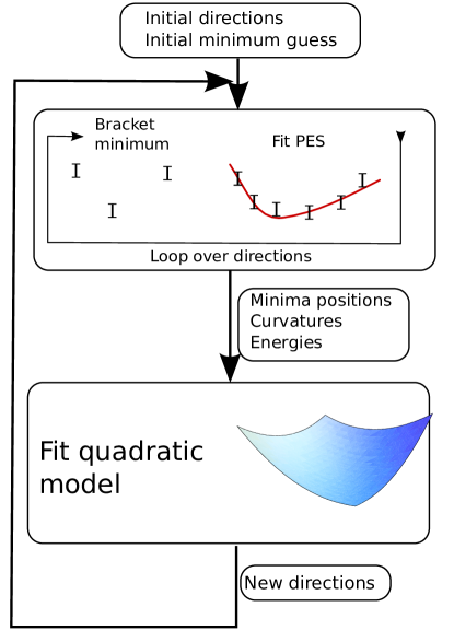
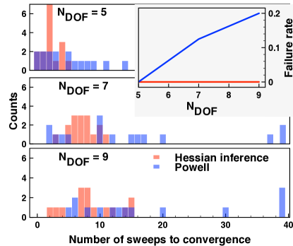
We outline a single iteration of the algorithm in Fig 1. This step operates in two principle regimes. The first is far away from the minimum. In this regime, the Hessian inference method behaves similarly to a deterministic direction set method, with the directions being determined by the Hessian inference. The second regime is when the calculation has mostly converged and the deterministic error in Eqn 2 is small compared to the stochastic error. In this regime, deterministic direction choices are particularly useless, but the inferred Hessian method is able to automatically account for the stochastic error. Once in this “stochastic regime,” we can use Eqn 3 to justify averaging the ’s to obtain a more precise estimate of the minimum. For stochastic functions, the performance of the Hessian inference is much higher than traditional methods such as Powell’s methodBrent (1973), which we compare in Fig 2. Since Powell’s method uses the concept of conjugate directions to find the search directions, the uncertain minimizations cause the algorithm to fail quickly. Even when the directions are reset every sweep, they can become linearly dependent within a single sweep, causing a high failure rate for even moderate dimensionality.
To show the value of optimizing geometries within QMC, we apply the method to the H2O-OH- complex (Fig 3), which is present in liquid water and important in many systems in condensed matter, biology, and chemistry. The shape of this potential energy surface is crucial to understanding hydrogen transfer in water. In this case, we use our knowledge of the system to choose fixed search directions for efficiency reasons, omitting the Hessian inference method. For systems that are not as easily decomposed, the Hessian inference is invaluable. It has been notedStaroverov et al. (2003) that current DFT functionals disagree on the ground state structure of this complex. The potential minima are the non-centrosymmetric structure (A) and the centrosymmetric structure (B).
Hartree-Fock and second order Møller-Plesset perturbation theory (MP2) find that structure A is lower in energy, with a barrier to transfer the proton. This is the traditional picture of this structure. The local density approximation and generalized gradient approximation (PBEPerdew et al. (1996)) of DFT find that structure B is lower in energy. Using our QMC line minimization method without constraints (seven degrees of freedom) we find structure A to be the minimum energy. The results are summarized in Table 1. DMC differs qualitatively from the DFT results in that structure A is the minimum, and quantitatively with MP2, since the oxygen-oxygen distance in MP2 is much smaller than in DMC for structure A.
| Method | O-O’ | O’-H | Structure type |
|---|---|---|---|
| LDA | 2.448 | 1.224 | B |
| PBE | 2.470 | 1.235 | B |
| MP2 | 2.469 | 1.123 | A |
| DMC | 2.491(2) | 1.111(3) | A |
| DMC* | 2.469(3) | 1.235(2) | B |
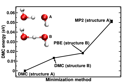
In Fig 3, we present the DMC energies of several minima. Without the geometry optimization algorithm, we would use minima from some other methods, for example, PBE and MP2 to obtain structures B and A respectively, then evaluate the total energy using DMC. In this case, since the MP2 approximation obtains a poor O-O distance, DMC predicts a much higher energy for structure A and thus favors the centrosymmetric geometry. However, this is qualitatively incorrect, as we can see from the DMC-optimized structures, which predict structure B to be about 0.015 eV higher in energy than structure A. It is notable that 0.015 eV is a very small energy difference on the scale of chemical bonding, which is why a small error in the geometry by using a lower level theory is enough to reverse the ordering. This energy difference is an upper bound to the barrier to transfer the hydrogen, and thus at room temperature the hydrogen is free to transfer between the oxygen atoms. This may have important implications for the development of effective solvent models for water.
In this work, we have viewed the DMC potential energy surface as a given without attempting to improve the accuracy over a simple Slater-Jastrow form; however, our method can also be used to optimize the nodal surface directly and thus further improve the accuracy of the DMC calculation. Similarly, any Monte Carlo method that depends on continuous parameters could put the stochastic line minimization algorithm to use. Stochastic line minimization may find application in experiments whose objective is to obtain a precise minimum in many-dimensional space, but the experiments are difficult to perform precisely. If it is instead easier to perform many iterations of the experiment, then the minimization method that we have outlined may be applicable. The scaling for a quadratic potential is if only values are used; if even approximate gradients are available, the scaling can be reduced to approximately , as discussed in the EPAPS document.
The algorithm is quite general, requiring only evaluations of the objective function with a known distribution, and can thus be applied to many minimization problems. At its core, it is a method for converting noisy value calculations into precise minima with rigorous error bounds, so it can be applied in any of the many problems where that is necessary. In electronic structure, diffusion Monte Carlo is accurate and applicable to many systems beyond the ground state of molecules, including solid structures and excited statesSchautz et al. (2004). The scaling for DMC geometry optimization is then , depending on the size of the system and whether gradients are available. This favorable scaling combined with the already known high accuracy of quantum Monte Carlo could open up new levels of accuracy in structure determination in condensed matter and chemical physics.
This work was supported by the Department of Energy under grant No. DE-SC0002623 and the NSF under grant No. 0425914. We wish to thank NERSC and Teragrid as well for providing computational resources. We would also like to acknowledge Yosuke Kanai for useful discussions.
References
- Kolorenč and Mitas (2008) J. Kolorenč and L. Mitas, Physical Review Letters 101, 185502 (pages 4) (2008), URL http://link.aps.org/abstract/PRL/v101/e185502.
- Grossman (2002) J. C. Grossman, The Journal of Chemical Physics 117, 1434 (2002), URL http://link.aip.org/link/?JCP/117/1434/1.
- Chiesa et al. (2005) S. Chiesa, D. M. Ceperley, and S. Zhang, Physical Review Letters 94, 036404 (pages 4) (2005), URL http://link.aps.org/abstract/PRL/v94/e036404.
- Assaraf and Caffarel (2003) R. Assaraf and M. Caffarel, J. Chem. Phys. 119, 10536 (2003).
- Casalegno et al. (2003) M. Casalegno, M. Mella, and A. Rappe, J. Chem. Phys. 118, 7193 (2003).
- Badinski and Needs (2007) A. Badinski and R. J. Needs, Physical Review E (Statistical, Nonlinear, and Soft Matter Physics) 76, 036707 (pages 10) (2007), URL http://link.aps.org/abstract/PRE/v76/e036707.
- Badinski et al. (2008) A. Badinski, J. R. Trail, and R. J. Needs, The Journal of Chemical Physics 129, 224101 (pages 7) (2008), URL http://link.aip.org/link/?JCP/129/224101/1.
- Filippi and Umrigar (2000) C. Filippi and C. J. Umrigar, Phys. Rev. B 61, R16291 (2000).
- Attaccalite and Sorella (2008) C. Attaccalite and S. Sorella, Physical Review Letters 100, 114501 (pages 4) (2008), URL http://link.aps.org/abstract/PRL/v100/e114501.
- Robbins and Monro (1951) H. Robbins and S. Monro, Ann. Math. Stat. 22, 400 (1951).
- Harju et al. (1997) A. Harju, B. Barbiellini, S. Siljamäki, R. M. Nieminen, and G. Ortiz, Phys. Rev. Lett. 79, 1173 (1997).
- Schuetz et al. (2003) C. A. Schuetz, M. Frenklach, A. C. Kollias, and J. W. A. Lester, The Journal of Chemical Physics 119, 9386 (2003), URL http://link.aip.org/link/?JCP/119/9386/1.
- Schmidt et al. (1993) M. W. Schmidt, K. K. Baldridge, J. A. Boatz, S. T. Elbert, M. S. Gordon, J. H. Jensen, S. Koseki, N. Matsunaga, K. A. Nguyen, S. J. Su, et al., J. Comput Chem 14, 1347 (1993).
- Burkatzki et al. (2007) M. Burkatzki, C. Filippi, and M. Dolg, The Journal of Chemical Physics 126, 234105 (pages 8) (2007).
- Thom H. Dunning (1989) J. Thom H. Dunning, The Journal of Chemical Physics 90, 1007 (1989), URL http://link.aip.org/link/?JCP/90/1007/1.
- Wagner et al. (2009) L. K. Wagner, M. Bajdich, and L. Mitas, Journal of Computational Physics 228, 3390 (2009), ISSN 0021-9991, URL http://www.sciencedirect.com/science/article/B6WHY-4VGPWS6-3/%2/df02c999649199aa85eb26ed66d87850.
- Adamo and Barone (1999) C. Adamo and V. Barone, The Journal of Chemical Physics 110, 6158 (1999), URL http://link.aip.org/link/?JCP/110/6158/1.
- Foulkes et al. (2001) W. M. C. Foulkes, L. Mitas, R. J. Needs, and G. Rajagopal, Rev Mod Phys 73, 1 (2001).
- Brent (1973) R. Brent, Algorithms for Minimization without Derivatives (Prentice-Hall, 1973), pp. 116–155.
- Staroverov et al. (2003) V. N. Staroverov, G. E. Scuseria, J. Tao, and J. P. Perdew, The Journal of Chemical Physics 119, 12129 (2003), URL http://link.aip.org/link/?JCP/119/12129/1.
- Perdew et al. (1996) J. P. Perdew, K. Burke, and M. Ernzerhof, Phys. Rev. Lett. 77, 3865 (1996).
- Schautz et al. (2004) F. Schautz, F. Buda, and C. Filippi, The Journal of Chemical Physics 121, 5836 (2004), URL http://link.aip.org/link/?JCP/121/5836/1.
Appendix A Details of the minimization algorithm
In this EPAPS document, we step through the minimization process in detail. Note that some of the details are not necessarily perfectly optimal, but they do work robustly and efficiently. We thus provide this description only as a reference implementation that could potentially be improved significantly.
A.1 Line minimization
Suppose we wish to minimize a function along a line using the values. For a deterministic function, a good method is the golden ratio method. However, for a non-deterministic function, locating the minimum by comparing the value is bound to be inefficient, since the objective function scales as , and the work to resolve energy differences scales as the inverse square root of the difference. Therefore, near the minimum, the effort to resolve position differences scales as the inverse quartic root of the difference. The computational cost using fitting (and gradients) on the other hand, scales as the inverse square root. Whether fitting using the value of the function or the gradient of the function is more accurate will depend on their relative variances and the specific problem. In this work, we use exclusively values since they are easily attainable in quantum Monte Carlo methods.
We developed a reliable strategy to bracket the minimum. Given a starting position () and a trust radius , the algorithm works with three points, initialized as follows: , , . Let be the function evaluated at with a normal random error with standard deviation , which can be controlled by performing longer calculations. Define as being true when is significantly different from , i.e., about four standard deviations away. A basic algorithm as follows:
-
1.
Evaluate , , and at uncertainty
-
2.
If and :
-
•
If and stop. We have bracketed the minimum.
-
•
If and , then set for , return to 1.
-
•
If and , then set for , return to 1.
-
•
-
3.
Else and return to 1.
This algorithm occasionally gets stuck when two points are roughly the same distance from the minimum and thus have nearly the same value. This can be ameliorated by searching between points when only two are insignificantly different.
Once the minimum is bracketed to within the trust region, we can then fill in points along the line and fit. The distribution of points is not very critical, so long as there are a few points far away from the minimum to determine the curvature and higher order parameters accurately. We typically use a four parameter cubic form: , which gives a good balance between being accurate, easy to fit, and few parameters. A quadratic form requires trust radii that are very small, reducing the efficiency of the algorithm. We perform the fit using Bayesian inference given the set of data . The likelihood function is given by
| (9) |
where
| (10) |
is the probability that we would have obtained the data given a set of parameters. The distribution of a given parameter can be found by taking the marginal distribution of , or for more speed at the cost of not knowing the uncertainty well, simply using the maximum likelihood estimator.
A.2 Hessian estimation
One begins by noting that near the minimum, the energy is described by a quadratic function:
| (11) |
Far away from the minimum, this is an approximation to speed up the minimum search. Near the minimum, we used this property to prove the average properties of the stochastic sequence of line minimizations. Recall that only the minimum of the line minimization must be in the quadratic region. With no further assumptions, we can estimate the Hessian (and full quadratic surface) given a collection of line minimizations, even in the presence of stochastic noise.
Let be the collection of all parameters for the quadratic region, the collection of line parameters for line . We wish to find , where D is the set of function evaluations, arranged in lines. By Bayes’ theorem, we know that
| (12) |
Since is not based on stochastic data, it is a delta function that forces to be consistent with as follows. In the quadratic region, , minimizing along a direction from a starting position gives the one-dimensional function
| (13) |
This gives the following constraints on each set of line parameters :
| (14) |
| (15) |
| (16) |
We thus only need to integrate over the variables in each line that are not specified by the above equations. We can replace the by the reduced line parameters . Since there are three constraints per line, the dimensionality of is three less than the dimensionality of . We can recover the full set of line parameters as a function of the quadratic parameters and the reduced line parameters; i.e.,
We eventually want the likelihood function for the quadratic parameters and the reduced line parameters: , where is the data. This is given by
| (17) |
where is given by Eqn 9.
The first estimate of the Hessian matrix is achieved by minimizing the violation of Eqn 15 from the line fits. The minimum of the quadratic model is estimated as the last minimum found in a line minimization, and the minimum energy similarly. The parameters are then optimized for maximum likelihood using a conjugate gradient optimization method. Finally, the parameters are randomized and reoptimized to get out of local maxima. We find that the maximum likelihood estimator is typically quite sufficient for determining search directions; it is not necessary to sample to find distributions.
Note that each line minimization places three constraints on and has a dimensionality of , so to make this a fully determined problem, line minimizations are needed. This is always smaller than the line minimizations necessary in Powell’s method, the standard in gradient-free minimization, with the additional benefit that the Hessian inference method is uncertainty-aware, which allows much higher efficiency when uncertainty can be traded for computational time.
If gradient information is available, then they can be integrated directly into the likelihood function from Eqn 17 as a simple product:
| (18) | ||||
where the likelihood function can be approximated as
| (19) | ||||
and is the covariance matrix between all the gradient components. The Hessian inference then becomes essentially a quasi-Newton algorithm that is uncertainty aware. Approximate gradients are also useful, since minima can be determined by using only the value to perform the line fits. In some instances, one can imagine elaborations of this where DFT or other approximations to the gradient are used to accelerate the minimum search.
A.3 A detailed look as the algorithm proceeds
-
1.
Start a line minimization sweep, for each direction
-
•
Bracket the minimum
-
•
Fill in data points within the trust region from the minimum
-
•
Fit the data points with a function
-
•
Update the minimum
-
•
Add fit to list of fits
-
•
-
2.
Prune list of fits to contain only the last sweeps
-
3.
Fit N-dimensional quadratic model to lines, find maximum likelihood
-
4.
Diagonalize Hessian
-
5.
Update directions
-
6.
Return to 1.
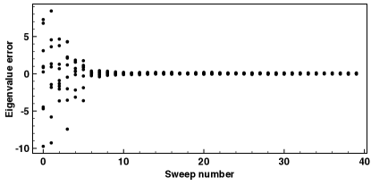
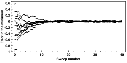
In Fig 4, we show the convergence of the eigenvalues from the Hessian estimation to the exact ones, and the minima from the line minimizations.
Appendix B Proofs of the properties of the stochastic sequence
We have the following equations:
| (20) |
| (21) |
Suppose that for some . Then , , and so on.
B.1 The average is equal to the true minimum
Suppose that . Then
| (22) |
This goes to zero exponentially in , so we can obtain an average arbitrarily close to zero by starting the average at high enough .
B.2 The average has finite variance
Assume . Then
| (23) |
for large .
B.3 The sequence has a finite correlation time
Suppose that
| (24) |
for some variance . Then the correlation between elements and in the sequence is
| (25) |
where we reversed the sum indices. As and become large while keeping the difference finite, we can then find that
| (26) |
This goes to zero exponentially with , and since the variance is finite, the correlation coefficient also goes to zero exponentially.