Anomalous localisation in the aperiodic Kronig-Penney model
Abstract
We analyse the anomalous properties of specific electronic states in the Kronig-Penney model with weak compositional and structural disorder. Using the Hamiltonian map approach, we show that the localisation length of the electronic states exhibits a resonant effect close to the band centre and anomalous scaling at the band edges. These anomalies are akin to the corresponding ones found in the Anderson model with diagonal disorder. We also discuss how specific cross-correlations between compositional and structural disorder can generate an anomalously localised state near the middle of the energy band. The tails of this state decay with the same stretched-exponential law which characterises the band-centre state in the Anderson model with purely off-diagonal disorder.
Pacs: 73.20.Jc, 73.20.Fz, 71.23.An
1 Introduction
The interest in one-dimensional random models has been constantly increasing since the discovery that, contrary to previous beliefs, systems of this class can undergo a sort of localisation-delocalisation transition when disorder exhibits specific long-range correlations [1]. Nowadays, one-dimensional models with correlated disorder are used in many fields of physics, including semiconductor superlattices [2], bilayered media [3], Bose-Einstein condensates [4], transmission in waveguides [5] and structures with corrugated surfaces [6], and DNA modelling [7].
In many of these problems, the system under study is represented in terms of an aperiodic Kronig-Penney model. The original Kronig-Penney model was introduced in the early 1930s to analyse the band structure of crystalline materials [8] and found new applications in the 1980s when it was used to study electronic states in semiconductor superlattices [9]. More recently, the interest in random one-dimensional systems has spurred investigations of the aperiodic variants of the Kronig-Penney model, which have been analysed both theoretically and experimentally [2, 5, 10].
Because of the simplicity and versatility of the aperiodic Kronig-Penney model, it is important to obtain as much analytical information as possible on the structure of its electronic states. A detailed study of the Kronig-Penney model with weak compositional and structural disorder was done in [11], where an analytical expression for the localisation length of the electronic states was derived. The formula works very well for most values of the energy, but fails in a neighbourhood of the band centre and of the band edges, where localisation anomalies appear. The first goal of the present work is to understand these anomalies: using the Hamiltonian map approach [12], we show that they have the same form of the corresponding anomalies which exist in the standard Anderson model with diagonal disorder at the band centre [13, 14] and at the band edge [15]. These anomalies have recently attracted attention because of the related violations of the single-parameter scaling hypothesis [16] at the edge [17] and at the centre [18] of the energy band. It is therefore of some interest to see whether similar anomalies exist in the random Kronig-Penney model.
After explaining the nature of the anomalies of the localisation length at the band centre and band edges, we focus our attention on a particular variant of the random Kronig-Penney model, characterised by specific cross-correlations between the compositional disorder and the structural one. We show that such a Kronig-Penney model corresponds to a Anderson model with energy-dependent diagonal and off-diagonal disorder. For a specific value of the energy, the diagonal disorder vanishes and the Kronig-Penney model becomes equivalent to the Anderson model with purely off-diagonal disorder. As is known [19], at the band centre the Anderson model with purely diagonal disorder has anomalously localised states, whose existence is another violation of the single-parameter scaling hypothesis [20]. Because of the identity of the mathematical equations, similar states with stretched-exponential tails also exist in the considered variant of the Kronig-Penney model.
This paper is organised as follows. In Sec. 2 we define the model under study and we summarise the main results concerning the localisation of the electronic states in the standard case. In Sec. 3 we discuss the anomalies of the localisation length emerging for values of the energy close to the band centre and in the neighbourhood of the band edge. In Sec. 4 we analyse the anomalously localised states created by particular cross-correlations of the disorder. The conclusions are drawn in Sec. 5.
2 Localisation of the electronic states: the standard case
In this section we define the model under study and we briefly derive the expression for the localisation length valid in the general case.
2.1 Definition of the model
We consider a Kronig-Penney model with weak compositional and structural disorder. The model is defined by the Schrödinger equation
| (1) |
which describes the motion of an electron of energy in a potential formed by a succession of aperiodically positioned delta-barriers of random strengths. To simplify the form of the equations, here and in what follows we use energy units such that . We introduce compositional disorder in model (1) by assuming that the barrier strengths display random fluctuations around their mean value . The structural disorder, on the other hand, is present because the positions of the barriers are displaced by a random amount with respect to the lattice sites .
For weak disorder, it is enough to specify the statistical properties of the model in terms of the first two moments of the strength fluctuations and of the relative displacements (which are more relevant than the absolute displacements themselves for the description of the electronic states). We assume that both variables have zero average, and , and that their variances satisfy the conditions of weak compositional disorder
and of weak structural disorder
| (2) |
We also consider the normalised binary correlators
| (3) |
as given functions. We do not attribute any specific form to the correlators (3); we only assume that, because of the spatial homogeneity in the mean of the model, they are (decreasing) functions of the difference of the site indices. For the sake of simplicity, we restrict our attention to the case in which the self-correlators and are even functions of , but we do not make the same assumption about the cross-correlator (in other words, we suppose that the model is only partially isotropic).
2.2 The Hamiltonian map approach
The Schrödinger equation (1) has the same form of the dynamical equation of a stochastic oscillator with frequency perturbed by a random succession of delta-shaped impulses (“kicks”). The Hamiltonian of such an oscillator is
| (4) |
The mathematical identity of the dynamical equation of the kicked oscillator (4) with Eq. (1) allows one to analyse the properties of the electronic states of the Kronig-Penney model (1) in terms of the trajectories of the kicked oscillator (4): this is the key idea of the Hamiltonian map approach [12, 21]. After integrating the Hamiltonian equations of the stochastic oscillator over the interval between two successive kicks, one obtains the Hamiltonian map
| (5) |
with the transfer matrix
| (6) |
To analyse the trajectories of the Hamiltonian map (5), we follow the approach proposed in [10] (see [11] for details) and we perform the canonical transformation of the form
| (7) |
The parameter in Eq. (7) is defined by the identity
The utility of the transformation (7) lies in the fact that the Hamiltonian map (5), when expressed in terms of the new variables , is reduced to a simple phase-space rotation in the absence of disorder. The rotation angle of the unperturbed map is defined by the identity
| (8) |
Eq. (8) determines the band structure of the Kronig-Penney model (1) and reveals that the parameter is the Bloch wavenumber.
To simplify the form of the Hamiltonian map (5) further, we switch from the Cartesian coordinates to action-angle variables via the standard relations
Within the second-order approximation, the Hamiltonian map (5) can be written in terms of the action-angle variables in the form [11]
| (9) |
with the ratio of the action variables being equal to
| (10) |
In Eqs. (9) and (10) we have introduced the rescaled disorder variables
| and | (11) |
and the parameter
| (12) |
2.3 The localisation length
The inverse localisation length for the Kronig-Penney model (1) is defined as
In the dynamical picture, is equivalent to the Lyapunov exponent of the Hamiltonian map (5),
| (13) |
with being defined by Eq. (10) and
| (14) |
As discussed in Sec. 3, in the weak-disorder case the invariant distribution for the angular variable is either flat (the normal case) or presents a moderate modulation (as happens at the band centre and for the other cases in which the Bloch wavenumber is a rational multiple of ). Only at the band edge the invariant distribution is strongly modulated even for weak disorder. Therefore as a function of the ratio (14) can be expected to oscillate around a unitary value, unlike the ratio which is larger than one on average because of the exponential increase of the action variable. As a consequence, away from the band edge, one can drop the second term in the right-hand side of Eq. (13) and compute the inverse localisation length as
| (15) |
Within the second-order approximation one can expand the logarithm in Eq. (15) and obtain
| (16) |
In the general case, the average over the angle variable in the right-hand side of Eq. (16) can be computed using a flat distribution . In fact, as the Hamiltonian map (9) shows, the angle variable has a fast dynamics compared to the action variable and quickly assumes a uniform distribution in the interval . In this way, following the steps of Ref. [11], one obtains that the inverse localisation length (15) has the form
| (17) |
with
Eq. (17) constitutes the standard expression of the inverse localisation length of the electronic states in the Kronig-Penney model (1). Note that expression (17) is slightly more general than the corresponding formula given in [11] because we have dropped the assumption that the cross-correlator is an even function of . The difference between the two expressions shows up in the last term of Eq. (17) and in the definition of the power spectrum. When , Eq. (17) reduces to the inverse localisation length derived in [11].
The inverse localisation length (17) works well for almost all values of the energy, but fails close to the band centre and at the band edges, where anomalous effects appear. The nature of these anomalies is discussed in the next section.
3 The band-centre and band-edge anomalies of the localisation length
As mentioned in the previous section, the derivation of formula (17) rests on the crucial assumption that the angle variable of the map (9) has a uniform invariant distribution. This assumption is generally justified on the grounds that the angle variable evolves much faster than the action variable and quickly sweeps the whole interval . One should notice, however, that this argument cannot be applied when the Bloch wavevector is a rational multiple of , because in this case the noiseless angular map has periodic orbits, whose effect persists in the form of a modulation of the invariant measure when a weak noise is switched on . For weak disorder, and within the limits of the second-order approximation, this implies that the general formula (17) cannot be applied when the Bloch vector takes values or , i.e., at the edges of the energy band, and for , i.e., for the energy which lies close to the band centre. In principle, one should expect anomalies for all Bloch vectors of the form with . In practice, however, in these cases the invariant distribution of the angular variable is modified by a perturbative term proportional to or and this does not affect the outcome of the average in Eq. (16), which contains only second- and fourth-order harmonics of (the same conclusion applies to the Anderson model, as discussed in Ref. [14]).
In conclusion, within the second-order approximation anomalies are found only at the band edge ( or ) or close to the middle of the band (). For these special values of the assumption of a flat invariant distribution must be abandoned and the specific form of has to be determined before one can compute the localisation length of the electronic states. The non-uniform distribution of the angular variable produces deviations from the standard formula (17) of the inverse localisation length; this section is devoted to the analysis of these anomalies.
For the sake of simplicity, in this section we will restrict our attention to the case of uncorrelated disorder. In other words, we will consider two successions of random variables and such that
In this case the standard expression (17) of the inverse localisation length reduces to the simple form
| (18) |
3.1 The anomaly near the middle of the energy band
We will first consider the anomaly for . The corresponding energy lies close to middle of the band and therefore we will often speak, somewhat loosely, of band-centre anomaly. By assigning the value to the Bloch vector and by taking into account that the noise-angle correlators vanish for uncorrelated disorder, one can reduce the general expression (16) to the simpler form
| (19) |
To determine the form of the invariant distribution , we follow the method introduced in [12] and we consider the map for the angle variable in Eq. (9) which, for uncorrelated disorder and , simplifies to
To get rid of the constant drift term, one can consider the fourth iterate of this map, i.e.,
Going to the continuum limit, one can replace this map with the Itô stochastic differential equation
| (20) |
where represent four independent Wiener processes. Given an initial condition , the Itô equation (20) defines a stochastic process , whose conditional probability can be obtained by solving the associated Fokker-Planck equation
| (21) |
with the initial condition [22]. The stationary solution of Eq. (21) which satisfies the conditions of normalisation and periodicity is [12]
| (22) |
In Eq. (22) is the complete elliptic integral of the first kind and we have introduced the constants
and
| (23) |
Eq. (22) shows that, as expected, when the Bloch vector takes the value , the invariant measure has period . The numerical computations agree well with formula (22) as can be seen in Fig. 1.
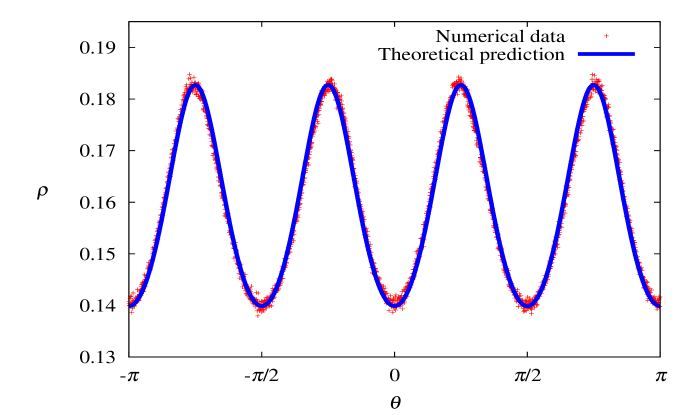
The data represented in Fig. 1 were obtained for mean field and disorder strengths . Here, and in the rest of the paper, we present numerical data which were obtained for energy values within the first band.
The knowledge of the invariant distribution (22) makes possible to compute the Lyapunov exponent (19). The averages of the functions of argument vanish, but the the average of does not and gives rise to the anomaly of the localisation length. After some algebra, one obtains that the inverse localisation length for is
| (24) |
where is the complete elliptic integral of the second kind and the argument is defined by Eq. (23). The numerical computations confirm the existence of an anomaly for as can be seen from the data represented in Fig. 2 which show a small but clear deviation from the value of the localisation length predicted by the standard formula (18).
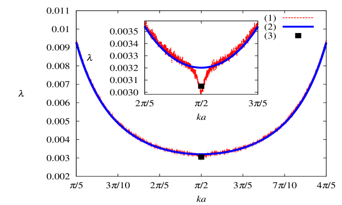
The numerically computed inverse localisation length for , on the other hand, matches well the theoretical value (24). We observe that the numerical data represented in Fig. 2 were obtained for a specific realisation of the disorder; when different disorder realisations are considered, the discrepancy between the numerical value of the Lyapunov exponent for and the predicted result (24) fluctuates slightly around zero, always assuming small values as in Fig. 2.
In conclusion, in the Kronig-Penney model (1) a resonance effect occurs for and produces an anomaly of the localisation length. The effect has the same nature of the band-centre anomaly found in the Anderson model with diagonal disorder [13, 12].
We remark that, although our analytical results are restricted to the case of uncorrelated disorder, we found numerical evidence that disorder correlations can enhance the anomaly of the localisation length near the middle of the energy band, in agreement with the theoretical conclusions of Ref. [23]. As an example, we can consider the case of structural and compositional disorder with self-correlations of the form
| (25) |
and no cross-correlations, . The long-range correlations of the form (25) create mobility edges at and (see [11] for details). Fig. 3 represents the numerical data obtained for this kind of disorder with and .
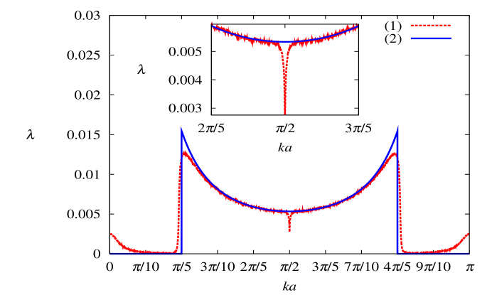
The data clearly show an enhanced anomaly at with respect to the case of totally uncorrelated disorder. Adding cross-correlations does not introduce any significant modification to the picture.
We would like to stress that, although the previous example shows how correlations of the disorder can enhance the anomaly for , not all correlations produce the same effect. This can be appreciated in the case analysed in Sec. 4, in which the resonance effect for is shadowed by a different kind of anomaly generated by specific cross-correlations for a value of close, but not identical, to .
3.2 The band-edge anomaly
We now turn our attention to the anomaly for , i.e., in the neighbourhood of the band edge. Because of the similarity with the band-edge anomaly in the Anderson model, we can apply the method used in [12] to the present case. We first derive the form taken by the map (9) at the band edge. For the rescaled random variables (11) can be approximated as
| and |
where we have introduced the symbol . In the same limit, the parameter (12) reduces to
| (26) |
Taking into account these approximations, one can write the Hamiltonian map (9) in the form
| (27) |
with
| (28) |
In Eqs. (27) and (28), the symbol represents the linear combination of structural and compositional disorder
with zero average, , and variance
Going to the continuum limit, one can replace the angular map in Eq. (27) with the stochastic Itô equation
| (29) |
whose associated Fokker-Planck equation
| (30) |
gives the conditional probability for the stochastic process [22]. By introducing the rescaled time
one can cast the Fokker-Planck equation (30) in the form
| (31) |
which contains the noise intensity and the distance from the band edge combined in the single scaling parameter
The invariant distribution is the stationary solution of the Fokker-Planck (31) which is normalisable and satisfies the periodicity condition . The solution possessing these features is [15, 12]
| (32) |
with
and
The integral representation (32) defines the invariant measure in the interval ; can be extended outside of this interval via the periodicity condition .
To obtain a qualitative understanding of the behaviour of the invariant distribution (32), it is useful to consider its values at the edges and at the centre of the interval. For and one has
while for the invariant distribution behaves as
These equations show that, when the energy moves closer to the band edge on the scale defined by the disorder strength, i.e., for , the invariant distribution develops two pronounced maxima for and . This conclusion is supported by direct numerical computation of the invariant distribution, as shown by Fig. 4.
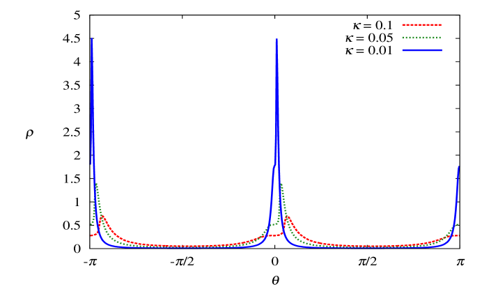
The data in Fig. 4 were obtained for mean field and disorder strengths .
The assumption of a uniform or slightly modulated distribution must therefore be radically dropped and this entails that one can no longer neglect the logarithm of the ratio (14) in the expression (13) of the inverse localisation length. Taking into account Eq. (26), in the neighbourhood of the band edge the inverse localisation length (13) can be reduced to the form
| (33) |
On the other hand, using the angular map in Eq. (27), one can write the sine ratio in Eq. (33) as
| (34) |
Substituting the approximate identities (28) and (34) in Eq. (33), one obtains
The average can now be computed using the invariant distribution (32); the final result is [12]
| (35) |
Away from the band-edge on the length scale set by the disorder strength, i.e., for , Eq. (35) reduces to
which coincides with the form of the standard expression (18) in the limit . On the other hand, close to the band-edge (on the length scale defined by the disorder strength), i.e., for , Eq. (35) gives
which exhibits the same anomalous scaling found in the Anderson model at the band-edge [15, 12]. This correspondence is a consequence of the fact that in both models at the band edge the invariant distribution for the angular variable has the form (32) and the ratio reduces to the same function of .
4 Existence of anomalously localised states in the Kronig-Penney model
In this section we discuss how specific cross-correlations between the two kinds of disorder (structural and compositional) can endow the Kronig-Penney model (1) with electronic states whose amplitude, away from the localisation centre , decays like a stretched exponential. More precisely, one has
| (36) |
where is a constant. This corresponds to a stretched exponential with stretching exponent . The phenomenon has its counterpart in the band-centre anomaly which occurs in the Anderson model with purely off-diagonal disorder [19].
As remarked in the previous section, the Kronig-Penney model (1) has an equivalent tight-binding model. The correspondence is easily established by eliminating the momenta from the map (5); in this way, with the obvious substitution , one obtains the equation
| (37) |
It is convenient to express the coefficients of Eq. (37) as sums of their mean values and of fluctuating terms with zero average. Eq. (37) then assumes the form
| (38) |
with being a deterministic function of the wavevector defined by the identity
| (39) |
while the symbols and stand for the energy-dependent random variables
| (40) |
and
| (41) |
Eq. (38) shows that the tight-binding counterpart of the Kronig-Penney model (1) is an Anderson model with both diagonal and off-diagonal disorder. Note that, in the absence of structural disorder, the random variables (40) vanish and the Kronig-Penney’s analogue becomes the ordinary Anderson model with diagonal disorder. For purely compositional disorder, therefore, one could have predicted a priori the existence of the anomalies discussed in Sec. 3.
We now focus our attention on the case in which the compositional disorder has the form
| (42) |
where represents the wavevector fulfilling the condition
| (43) |
We stress that condition (42) introduces special cross-correlations between the two kinds of disorder in the Kronig-Penney model (1). We also remark that the weak-disorder condition (2) ensures that a solution of Eq. (43) exists. In fact, taking into account the band-structure relation (8), within the limits of the second-order approximation one can cast Eq. (43) in the form
If the structural disorder is weak enough, the right-hand side of this equation is less than one and this implies that a Bloch vector exists such that is the solution of Eq. (43). Actually, a perturbative calculation shows that the Bloch vector in the positive half of the first Brillouin zone is
| (44) |
with . For weak disorder the deviation of from is not large and therefore , which is close to centre of the energy band.
If the compositional disorder has the form (42), it is easy to see that, when the electron energy takes the critical value identified by the condition (43), Eq. (38) becomes
| (45) |
which has the same form of the Schrödinger equation for the Anderson model with purely off-diagonal disorder and zero energy. For zero energy, the latter model is known to have an electronic state which exhibits anomalous localisation, because it is localised but decays away from the localisation centre according to Eq. (36) [19]. We stress that the identity of Eq. (45) with the zero-energy Schrödinger equation for the Anderson model with only off-diagonal disorder ensures that, when the compositional disorder has the form (42) and the energy takes the critical value , the Kronig-Penney model also has an anomalously localised state whose amplitude decays exponentially with the square root of the distance from the localisation centre.
This property can be heuristically justified with the observation that Eq. (45) implies that
| (46) |
By invoking the central limit theorem, one can therefore conclude that, for large values of , the random variable has zero average and a variance which increases linearly with . We stress that the previous argument holds even if the disorder exhibits long-range self-correlations of the form
| (47) |
where and are real numbers such that . In fact, weaker forms of the central limit theorem can be applied to sums of correlated random variables, provided that the correlations decay fast enough [24, 25]. Specifically, given a succession of zero-average, correlated random variables , let be the sum of the first terms of the succession. The minimal condition for the mean square of to grow linearly with , i.e., , is that the power spectrum of the succession be finite at the origin. The power spectrum corresponding to the binary correlator (47) is
| (48) |
and vanishes at the origin; one can therefore conclude from Eq. (46) that
even if the disorder is correlated.
The numerical data confirm the conclusion that the Kronig-Penney model (1) has an anomalously localised state for when the compositional disorder takes the special form (42). This can be seen from Figs. 5 and 6, which show how the Lyapunov exponent vanishes when the Bloch wavevector takes the critical value .
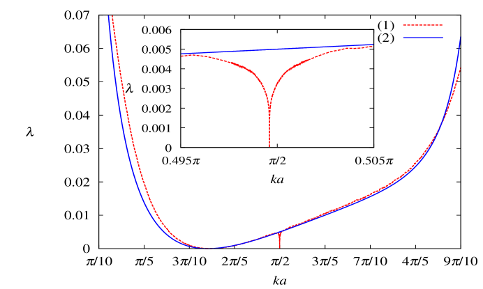
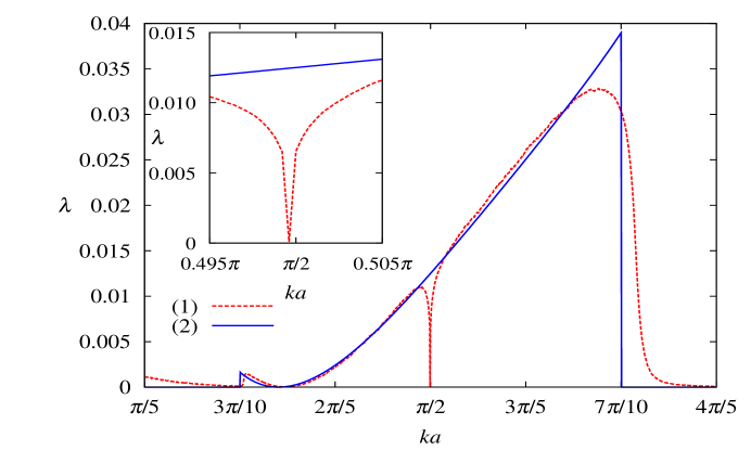
The difference between Figs. 5 and 6 lies in the fact that in the case corresponding to Fig. 5 the structural disorder is not self-correlated, while the data represented in Fig. 6 were obtained for structural disorder with long-range self-correlations of the form (47) with and .
All the numerical data presented in this section were obtained for a Kronig-Penney model with mean field and structural disorder characterised by a uniform distribution
| (49) |
with width , corresponding to a disorder strength . For the above-specified values of the mean field and of the disorder strength, formula (44) gives a value of the critical Bloch wavevector approximately equal to , in relatively good agreement with the numerically obtained value .
When the box distribution (49) is chosen for the displacements , the function (39) becomes
| (50) |
while the random variables (40) and (41) take the forms
| (51) |
and
| (52) |
We would like to stress that, when performing numerical calculations, one should work with the exact form (50) of and the exact expressions (51) and (52) of the coefficients and , even if the disorder is weak. Obviously, the explicit expressions of these magnitudes depend on the distribution chosen for the variables and must be modified if the box distribution is replaced with another one. Whatever distribution is adopted, however, it is important that the corresponding exact expressions of , and be used. Using second-order approximations for and the random coefficients (41) works relatively well for most values of the energy, but fails at the critical point, because the neglected higher-order corrections produce non-zero diagonal terms in Eq. (38) which, in spite of being very small, prevent the electronic state from being anomalously localised and the Lyapunov exponent from vanishing completely.
As a side remark, we would like to add that the conditions (42) and (43) ensure the existence of an anomalously localised state also for disorder of arbitrary strength, provided that Eq. (43) has a solution inside the allowed energy bands. This is confirmed by numerical calculations (which, incidentally, also show that when disorder is not weak the critical value of the energy need not be close to the band centre). To determine the conditions which guarantee the existence of such a critical value of the energy in the general case is not an easy task, however; for the sake of simplicity, we therefore restrict our attention to the case of weak disorder, for which the band structure is approximately given by Eq. (8) and Eq. (43) does have a solution.
In both Fig. 5 and 6 the numerical data are compared with the theoretical predictions derived from the general result (17). Because in this formula terms of order higher than the second are neglected, in its evaluation we replaced the exact expression (42) of the compositional disorder with its second-order approximation
| (53) |
In passing, we observe that Eq. (53) implies that the cross-correlator is not an even function of its argument. When the compositional disorder has the form (53), the inverse localisation length (17) becomes
| (54) |
The power spectrum in the previous formula reduces to in the case of uncorrelated structural disorder, while it is of the form (48) in the case of self-correlated structural disorder represented in Fig. 6. Note that in the latter case the long-range correlations (47) create two mobility edges at and . As can be seen from Figs. 5 and 6, the theoretical formula (54) works reasonably well everywhere, except in a small neighbourhood of the critical value . This failure must be ascribed to the fact that Eq. (54), as its parent expression (17), is not valid for Bloch wavevectors lying close to the rational value , where resonance effects play a non-negligible role.
As a last comment on the specific features of the localisation length in the special case in which the compositional disorder is related to the structural one by Eq. (42), we observe that Eq. (54) predicts the existence of a delocalised state for the Bloch wavevector identified by the condition
This is confirmed by the numerical computations, as can be seen from both Figs. 5 and 6.
To conclude this section, we would like to add some numerical evidence of the stretched-exponential behaviour of the tails of the anomalously localised state. We have numerically solved Eqs. (38) and (45) as initial-value problems; this corresponds to constructing the electronic states with the transfer-matrix technique. In the anomalous case one expects to behave as the position of a random walker, i.e., as a random variable with constant zero average and a second moment linearly increasing with . For , on the other hand, the solution of Eq. (38) should behave as , leading to an increase with of the -th moment of . This is confirmed by the numerical data for the first two moments of the variable , represented in Figs. 7 and 8.
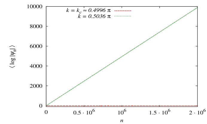
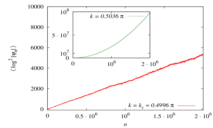
In both Figs. 7 and 8 we considered the behaviour of as a function of for two Bloch wavevectors, i.e., the critical vector and the vector , which is close to the critical value but not identical to it. The moments of were computed with an average over 1000 disorder realisations. For the sake of simplicity, we considered compositional disorder without self-correlations. Both the first and the second moment of behave as expected, corroborating the conclusion that the tails of the electronic state at the critical point are described by Eq. (36).
5 Conclusions
In this work we analyse the anomalous behaviour of specific electronic states in the Kronig-Penney model with weak compositional and structural disorder. In every case we discuss the analogies with the corresponding phenomena in the Anderson model.
We first show that the localisation length deviates from the prediction of the standard formula (17) when the Bloch vector assumes the value , which corresponds to an energy close to the band centre. This discrepancy is due to the same resonance effect which occurs in the standard Anderson model at the band centre; in both models this effect produces a modulation of period of the invariant distribution of the angle variable of the associated Hamiltonian map. This modulation leads to the band-centre anomaly of the localisation length.
We make use of the Hamiltonian map approach also to analyse the electronic states at the band edge. We find again that the same anomalous behaviour originally found in the Anderson model is present in the Kronig-Penney model. In both systems the most relevant feature at the band edge is the anomalous scaling of the localisation length with the disorder strength.
We finally use the correspondence between the Kronig-Penney model and the Anderson model with diagonal and off-diagonal disorder to conclude that in the former system specific cross-correlations between the two kinds of disorder generate an electronic state, close to the band centre, whose tails decay as stretched exponentials. This state is the analogue of the anomalously localised state which occurs at the band-centre in the Anderson model with purely off-diagonal disorder.
J. C. H.-H. and L.T. gratefully acknowledge the support of the CONACyT grant No. 84604 and of the CIC-2009 grant (Universidad Michoacana). The work of F.M.I. was partly supported by the CONACyT grant No. 80715.
References
- [1] F. A. B. F. de Moura, M. L. Lyra, Phys. Rev. Lett. 81, 3735 (1998); F. A. B. F. de Moura, M. L. Lyra, Phys. Rev. Lett. 84, 199 (2000); F. M. Izrailev, A. A. Krokhin, Phys. Rev. Lett. 84, 4062 (1999)
- [2] V. Bellani, E. Diez, R. Hey, L. Toni, L. Tarricone, G. B. Parravicini, F. Domínguez-Adame, R. Gómez-Alcalá, Phys. Rev. Lett. 82, 2159 (1999); A. Esmailpour, M. Esmaeilzadeh, E. Faizabadi, P. Carpena, M. Reza Rahimi Tabar, Phys. Rev. B 74, 024206 (2006)
- [3] F. M. Izrailev, N. M. Makarov, Phys. Rev. Lett. 102, 203901 (2009)
- [4] L. Sanchez-Palencia, D. Clément, P. Lugan, P. Bouyer, G. V. Shlyapnikov, A. Aspect, Phys. Rev. Lett. 98, 210401 (2007); P. Lugan, A. Aspect, L. Sanchez-Palencia, D. Delande, B. Grémaud, C. A. Müller, C. Miniatura, Phys. Rev. A 80, 023605 (2009); P. Bouyer, Ann. Phys. (Berlin) 18 844 (2009)
- [5] U. Kuhl, F. M. Izrailev, A. A. Krokhin, H.-J. Stöckmann, Applied Phys. Lett. 77, 633 (2000); A. Krokhin, F. Izrailev, U. Kuhl, H.-J. Stöckmann, S. E. Ulloa, Physica E 13, 695 (2002); F. M. Izrailev, N. M. Makarov, Phys. Rev. B 67 113402 (2003); U. Kuhl, F. M. Izrailev, A. A. Krokhin, Phys. Rev. Lett. 100, 126402 (2008); G. A. Luna-Acosta, F. M. Izrailev, N. M. Makarov, U. Kuhl, H.-J. Stöckmann, Phys. Rev. B 80, 115112 (2009)
- [6] F. M. Izrailev, N. M. Makarov, Phys. Rev. B 67 113402 (2003); F. M. Izrailev, N. M. Makarov, M. Rendón, phys. stat. sol. (b) 242, 1224 (2005)
- [7] A. A. Krokhin, V. M. K. Bagci, F. M. Izrailev, O. V. Usatenko, V. A. Yampol’skii, Phys. Rev. B 80, 085420 (2009); E. L. Albuquerque, M. L. Lyra, F. A. B. F. de Moura, Physica A 370, 625 (2006)
- [8] R. de L. Kronig, W. G. Penney, Proc. Roy. Soc. (Series A) 130, 499 (1931)
- [9] J. H. Davies, The physics of low-dimensional semiconductors: an introduction, Cambridge University Press, Cambridge (1998)
- [10] F. M. Izrailev, A. A. Krokhin, S. E. Ulloa, Phys. Rev. B 63, 041102(R) (2001)
- [11] J. C. Hernández Herrejón, F. M. Izrailev, L. Tessieri, Physica E 40, 3137 (2008); J. C. Hernández-Herrejón, F. M. Izrailev, L. Tessieri, arXiv:1003.3691
- [12] F. M. Izrailev, S. Ruffo, L. Tessieri, J. Phys. A: Math. Gen., 31, 5263 (1998)
- [13] M. Kappus, F. Wegner, Z. Phys. B - Condensed Matter 85, 15 (1981)
- [14] C. J. Lambert, Phys. Rev. B 29, R1091 (1984)
- [15] B. Derrida, E. Gardner, J. Phys. (Paris) 45, 1283 (1984)
- [16] E. Abrahams, P. W. Anderson, D. C. Licciardello, T. V. Ramakrishnan, Phys. Rev. Lett. 42, 673 (1979)
- [17] L. I. Deych, A. A. Lisyansky, B. L. Altshuler, Phys. Rev. Lett. 84, 2678 (2000); L. I. Deych, A. A. Lisyansky, B. L. Altshuler, Phys. Rev. B 64, 224202 (2001); L. I. Deych, M. V. Erementchouk, A. A. Lisyansky, Phys. Rev. B 67, 024205 (2003); H. Schomerus, M. Titov, Phys. Rev. E 66, 066207 (2002)
- [18] H. Schomerus, M. Titov, Phys. Rev. B 67, 100201(R) (2003); L. I. Deych, M. V. Erementchouk, A. A. Lisyansky, B. L. Altshuler, Phys. Rev. Lett. 91, 096601 (2003)
- [19] F. Dyson, Phys. Rev. 92, 1331 (1953); G. Theodorou, M. H. Cohen, Phys. Rev. B 13, 4597 (1976); L. Fleishman, D. C. Licciardello, J. Phys. C: Solid State Phys. 10, L125 (1977); T. P. Eggarter, R. Riedinger, Phys. Rev. B 18, 569 (1978); C. M. Soukoulis, E. N. Economou, Phys. Rev. B 24, 5698 (1981); P. Markos̆, Z. Phys. B-Condensed Matter, 73, 17 (1988); A. Bovier, Journ. Stat. Phys., 56, 645 (1989); M. Inui, S. A. Trugman, E. Abrahams, Phys. Rev. B, 49, 3190 (1994); H. Cheraghchi, S. M. Fazeli, K. Esfarjani, Phys. Rev. B, 72, 174207 (2005)
- [20] H. Cheraghchi, J. Stat. Mech., P11006 (2006)
- [21] F. M. Izrailev, T. Kottos, G. P. Tsironis, Phys. Rev. B, 52, 3274 (1995)
- [22] C. W. Gardiner, Handbook of Stochastic Methods, 3rd ed., Springer Verlag, Berlin (2004)
- [23] M. Titov, H. Schomerus, Phys. Rev. Lett. 95, 126602 (2005)
- [24] Shang-Keng Ma, Statistical Mechanics, World Scientific, Singapore, (1985)
- [25] A. C. Davison, D. R. Cox, Proc. R. Soc. Lond. A, 424, 255-262 (1989)