Optimization Under Unknown Constraints
Abstract
Optimization of complex functions, such as the output of computer simulators, is a difficult task that has received much attention in the literature. A less studied problem is that of optimization under unknown constraints, i.e., when the simulator must be invoked both to determine the typical real-valued response and to determine if a constraint has been violated, either for physical or policy reasons. We develop a statistical approach based on Gaussian processes and Bayesian learning to both approximate the unknown function and estimate the probability of meeting the constraints. A new integrated improvement criterion is proposed to recognize that responses from inputs that violate the constraint may still be informative about the function, and thus could potentially be useful in the optimization. The new criterion is illustrated on synthetic data, and on a motivating optimization problem from health care policy.
Key words: constrained optimization, surrogate model, Gaussian process, sequential design, expected improvement
1 Introduction
A common optimization problem that arises in fields ranging from applied engineering to public policy is to find , subject to constraints: , where we may only learn about the relationship between and and the constraint region through expensive evaluations of the noisy joint process
| (1) | ||||
The real-valued noise variance, , is unknown but may be zero, and indicates that the constraint mapping may be random. In particular, the constraint region is well-defined but often non-trivial. Although it will typically be deterministic (), this is not required by our treatment. Finally, we suppose that observing the joint response is expensive. So we wish to keep the number of evaluations, , small. One way to do this is to build regression and classification models for and for based on the data. The surrogate surfaces may be searched to find yielding a small objective in expectation, and satisfying the constraint with high probability. We can then repeat the process with points, including , stopping when convergence in the location of is achieved, or when resources are exhausted.
To shed light upon the difficulty in solving this problem, and to thereby suggest possible points of attack, consider the following simplification where the constraint region is known at the outset (i.e., there is no need to estimate ). In this case a sensible approach is as follows. Obtain realizations of only for with the largest expected improvement (EI, Jones et al.,, 1998) under [more on this in Section 2] and proceed to construct by adding the pair into the design. This presumes that evaluating for is a waste of resources. But this need not be so, since , for any , contains information about , and therefore about promising location(s) for . It could even be that is best at reducing the overall uncertainty in the location of , through an improved new surrogate . When this is the case [e.g., see Section 3.3] it makes sense to sample for despite the constraint violation.
Assessing when this odd maneuver is advantageous requires a more global notion of improvement; EI cannot directly quantify the extent to which improves our information at . Finally, when is not known a priori, new evaluations provide information about both and through their surrogates and . Thus incremental decisions toward solving the constrained optimization problem must incorporate uncertainty from both surrogates. We propose a new integrated improvement statistic to fit the bill.
The rest of the paper is outlined as follows. In Section 2 we outline EI for (unconstrained) optimization and the GP surrogate models upon which it is based. In Section 3 we develop the conditional and integrated expected improvement statistic(s) for the case of known constraints, with an illustration. We extend the method to unknown constraints in Section 4, and demonstrate the resulting constrained optimization algorithm on synthetic data. In Section 5 we consider a motivating problem from health care policy research, and conclude with some discussion and extensions in Section 6. Software implementing our methods, and the specific code for our illustrative examples, is available in the plgp package (Gramacy,, 2010) for R on CRAN.
2 Previous Work
2.1 Surrogate Modeling
The canonical choice of surrogate model for computer experiments is the stationary Gaussian process (GP, Sacks et al.,, 1989; O’Hagan et al.,, 1999; Santner et al.,, 2003), which is one way of characterizing a zero mean random process where the covariance between points is explicitly specified through the function . Let be the vector of observed observed responses at the design points collected (row-wise) in . Conditional on this data , the (posterior) predictive distribution of at a new point under the GP is normal with
| mean | (2) | ||||
| and variance |
where is the -vector whose component is , and is the matrix with element . These are sometimes called the kriging equations. Joint prediction at a collection of points is multivariate normal with mean vector and covariance matrix which are defined by the straightforward matrix extension of and . We follow Gramacy and Lee, (2008) in specifying that have the form where is the Kronecker delta function, and is a true correlation function. The term, referred to as the nugget, is positive and provides a mechanism for introducing measurement error into the stochastic process—implementing in Eq. (1) (Gramacy,, 2005, appendix). It causes the predictive equations (2) to smooth rather than interpolate the data . It is common to take from a parametric family, such as the separable Matérn or power families (e.g., Abrahamsen,, 1997), which roughly model as an inverse function of coordinate-wise Euclidean distance. We prefer the power family, which is standard for computer experiments.
2.2 Optimization by Expected Improvement
Conditional on a GP surrogate , a step towards finding the minimum may be based upon the expected improvement (EI) statistic (Jones et al.,, 1998). For a deterministic function (), the current minimum is deterministic. In this case, the improvement is defined as . The next location is chosen as
| (3) |
where the expectation is taken over , the predictive distribution (2) implied by evaluated at . Jones et al., (1998) give an analytical expression for the EI:
| (4) |
Basically, the EI is the cumulative distribution of the predictive density that lies “underneath” . A relevant diagram illustrating EI appears in Figure 1 in Section 3.1.1. Jones et al., (1998) also provide a branch and bound algorithm for performing the maximization over to find . Once is chosen it is added into the design as and the procedure repeats with . Jones et al., (1998) use maximum likelihood inference to set the parameters for , i.e., only since , and call the resulting iterative procedure the efficient global optimization (EGO) algorithm. The above choice of is sensible but somewhat arbitrary. Another reasonable choice that we promote in this paper is , the minimum of the (posterior) mean predictive surface.
The situation is more complicated for noisy responses. We must then estimate the nugget, , and extend the Jones et al., (1998) definition of to be a random variable: the first order statistic of . Calculating the EI would thus require integrating over in Eq. (3). This breaks the analytical tractability of EGO algorithm, however one can always proceed by Monte Carlo methods. Once in the Monte Carlo framework, extensions abound. For example, it is trivial to take a Bayesian approach and thereby factor parameter uncertainty into the EI calculation. Conditional on the parameters however, choosing is still deterministic. So this choice allows an analytical approach to proceed when point-estimates (i.e., MLEs) of parameters are used, or it leads to a more efficient Monte Carlo algorithm when sampling from the Bayesian posterior. The downside of the Monte Carlo approach, whether taken for Bayesian or considerations, is that the branch and bound algorithm for determining in Eq. (3) is no longer available. However, proceeding with a discrete set of space-filling candidates, and leveraging direct optimization methods in tandem, has proved fruitful (Taddy et al.,, 2009b).
2.3 Towards Constrained Optimization
Ours in not the first attempt at tackling the constrained optimization problem via surrogate modeling. Schonlau et al., (1998) consider deterministic responses () where the known constraint region can be written as , for . They then treat the as additional response variables that co-vary with . This breaks the analytical tractability of the EI calculation. Upon assuming that the responses are independent the calculation is again tractable, otherwise a Monte Carlo approach is needed. We are not aware of any previous literature addressing our more general problem: where the function may not be deterministic, and when there are unknown constraints of arbitrary form. Even in simpler settings, like the one above, it may be advantageous to sample outside the constraint region. This requires a new improvement statistic—one that weighs the overall expected improvement of the next sequentially chosen design point in aggregate.
3 Integrated Expected Conditional Improvement
Here we generalize the EI framework to accommodate the drawbacks outlined above. To start with, we assume that constraints are deterministic, and known (with trivial computation) in advance. Section 4 provides extensions for unknown constraints.
Define the conditional improvement as
| (5) |
where , which is the predictive distribution of the response at a reference input location under the surrogate model given that the candidate location is added into the design. We do not use an subscript for the posterior predictive distribution because the realization of the response is not yet available.
The expected conditional improvement (ECI) at the reference point is then . Here the expectation is over all of the random quantities: the distribution of , and perhaps of depending upon how it is defined. The ECI may be evaluated at all pairs of inputs . The potential to generalize EI, which accounts for improvement at the point alone, comes by integrating over the choices for . Let denote a density over which may be uniform in a bounded region. Then the integrated expected conditional improvement (IECI) is defined as
| (6) |
This suggests using as the next adaptively sampled point. As long as for all , this statistic (6) is defensible. Defining carefully [see Section 3.1.1] ensures that this monotonicity condition holds.
The negation in Eq. (6) keeps IECI in line with the convention of maximizing, i.e., of preferring large EI statistics over small ones. To explain, consider how “looks ahead”. We wish to measure an improvement at , but in a roundabout way we assess that improvement at a reference point instead, supposing has been added into the design. If still has high improvement potential after has been added in, then must not have had much influence on the improvement at . If is influential at , then the improvement at should be small after is added in, not large.
We can alternatively define IECI as the expected reduction in improvement at the reference location, , when is added into the design:
| (7) |
which is guaranteed to be positive under our monotonicity assumption. We would then take the which gave the largest reduction. But clearly this is within an additive constant (the weighted-average EI over ) of the definition given in Eq. (6), and is thus equivalent.
The integrated approach allows constraints to be handled through . E.g., can be uniform for and zero otherwise. Or, [as we discuss in Section 4] it can give higher weight to with a greater chance of satisfying the constraint. When there are no constraints, choosing uniform on yields an aggregated statistic that will offer a more global search, compared to EI, in a manner similar to how the expected reduction in variance generalizes the predictive variance for sequential design by active learning (Seo et al.,, 2000; Gramacy and Lee,, 2009).
3.1 Expected Conditional Improvement
The key ingredient in calculating the ECI is an assumption about how behaves relative to . Let denote the distribution of . Overloading the notation somewhat, let denote the density of under , and likewise for . By the law of total probability,
| (8) | ||||
where is the predictive density of when the design matrix and response vector are augmented by . Note that the above expressions involving have an implicit conditioning upon . For an arbitrary surrogate, computing the integral in Eq. (8) analytically would present a serious challenge. However, under a GP surrogate it is trivial since and are both (univariate) normal distributions (2), and a convolution of normals is also normal. Trivially, the mean and variance of the (normal) predictive density is unchanged after integrating out since the GP is not dynamic, so there is no update from without observing .
But at the same time, the predictive variance (2) does not depend upon the responses, or via . So we can deduce what the variance of the predictive density will be once arrives. We will have under the assumption that the evidence in does not update/change parameters of the GP (which it can’t if it is not observed!). Now, depends upon whose row and column are populated with for and with appearing in the bottom right-hand corner. So can then be obtained in terms of via partitioned inverse equations. If
where and . This saves us from performing any additional matrix operations. So where is an -vector whose first entries are identical to and with an entry of . The amount by which is reduced compared to is then readily available. Let . Then,
| (9) | ||||
So we can see that the deduced predictive variance at will be reduced when is observed by an amount that depends upon how far apart and are. This is not only sensible, but will also be helpful for determining the influence of in improvement calculations.
To sum up, we propose to define , for the purposes of sequential design, to be a normal distribution with (true) mean and deduced variance as given in Eq. (9), above. As with the kriging equations (2), joint sampling for a collection of () reference inputs is possible via the appropriate matrix extensions to and in order to derive and .
Now, with an appropriate definition of a deterministic , the same analytic expression for the EI from Section 2 can be extended to the ECI:
| (10) | ||||
If we cared only about the ECI (without integration (6)), the branch and bound algorithm given by Jones et al., (1998) would apply leading to a conditional EGO algorithm.
3.1.1 Choosing
Figure 1 illustrates how a deterministic choice of can influence the ECI. Consider two cases ((a) and (b)), which pertain to the choices for introduced in Section 2.2 (represented by horizontal lines): (a) uses only the observed locations and (b) uses the whole predictive curve. We will return to details of these choices shortly. In the figure, the solid parabolic curve represents the predictive mean surface . The EI is the area of the predictive density drawn as a solid line, plotted vertically and centered at , which lies underneath the horizontal line(s), representing choices of .
The ECI is likewise the area of the predictive density drawn as a dashed line lying below the horizontal line(s). This dashed density has the same mean/mode as the solid one, but it is more sharply peaked by the influence of . If we suppose that the densities, drawn as bell-curves in the figure, are symmetric (as they are for a GP), then it is clear that the relationship between ECI and EI depends upon . As the dashed line is more peaked, the left-tail cumulative distributions have the property that for all , to which choice (a) for corresponds. Therefore in this case, violating our desired monotonicity property. But for choice (b) the ECI represents a reduction compared to the EI, since , thus satisfying the monotonicity property.
Case (a) in Figure 1 is meant to represent taking , deterministically. It may similarly represent the minimum of the mean-predictive at the locations, which would coincide with the minimum of the values in the no-noise () case. In the noisy case () in Eq. (5) is a random variable whose distribution can be approximated by simulation from . But this extra computational effort would be in vain because the monotonicity property is not guaranteed. Case (b) corresponds to taking , the minimum of the posterior mean-predictive—another deterministic choice. In this case it is clear that will always cut through the density of at or below its mean/mode and ensure that the monotonicity property is satisfied. Accordingly, we shall use this choice throughout the remainder of the paper.
3.1.2 A Monte Carlo Approach for Calculating the ECI
The following procedure may be used to obtain samples of the ECI via the GP surrogate posterior predictive , taking full account of uncertainty in the parameters . The procedure is borne out via Monte Carlo sampling for in Figure 2.
For , current design , repeat:
1.
Sample from the posterior distribution
conditional upon , priors, and , and possibly conditional
upon in an MCMC setup
2.
Calculate
3.
Obtain the sample from as
, following Eq. (10) with and
If is considered known, or has been estimated offline, e.g., via maximum likelihood, then we may skip the loop (and Step 1), taking with . In either case, an estimate of the ECI is obtained by ergodic averaging:
| (11) |
3.2 Integrated Expected Conditional Improvement Algorithm
Calculating the IECI (6) from the ECI requires integrating over according to , which may be uniform in a bounded (constraint) region. It will not generally be possible to integrate analytically, so we propose to augment the Monte Carlo procedure from Section 3.1.2. Given a large number of sampled reference locations , the IECI may be approximated with Monte Carlo samples from the ECI as follows.
| (12) |
When the parameters are known, as before. With larger (and ) we obtain an improved approximation, and in the limit we have equality. In the case where is uniform over a convex region, a grid or maximum entropy design may be preferred (Santner et al.,, 2003, Section 6.2.1). When the marginals of are known, a Latin Hypercube Design (LHD, Santner et al.,, 2003, Section 5.2.2) may be more generally appropriate.
If we choose (or are required) to work with a size grid, design, or LHD of reference locations , we may view as discrete and finite measure. An alternate approach in this case is to forgo (re-)sampling from and compute a weighted average instead:
| (13) |
This has the disadvantage that the ECI may be evaluated at many reference locations with low (or zero) probability under . But it has the advantage of an implementation that is easily adapted to the unknown constraint situations described shortly.
3.3 Illustrating IECI
To illustrate IECI consider the following process , observed for . As a mixture of a sinusoid and normal density function (with and ) it has two local minima in this region. To make things interesting, realizations of the process are observed with i.i.d. noise so that Var. The top-left panel of Figure 3 shows one random realization of this process at LHD inputs.
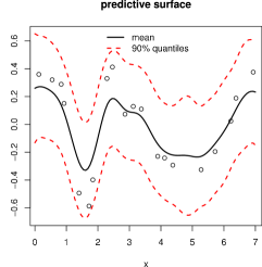
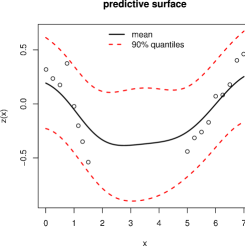
The predictive mean and 90% interval obtained by sampling from the posterior under the GP is also shown. A visual inspection of the surface(s) reveals that, indeed, there are two local minima.
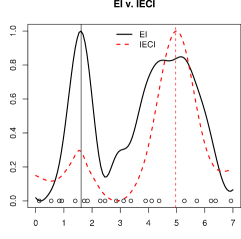
Below that panel, on the bottom-left, the EI (solid black) and IECI (dashed red) surfaces are plotted, normalized to appear on the same scale. As a further visual aid, the design is also shown, and the vertical lines crossing the -axis intersect with the curves at their maxima. We took a uniformly spaced set of 100 candidate locations in , our , and calculated the EI and IECI at . Likewise, we took the same points as reference locations for the IECI calculations via Eq. (12). EI recommends taking a sample from the left local minima, although the relative heights of the two disparate regions of highest EI betrays that this decision is indeed a “close call”. In contrast, IECI suggests taking the next sample from the right local minima, and with much greater decisiveness. The lower concentration of samples nearby this right-minima lead to higher variance in that region which may be pooled by the more globally-scoped IECI.
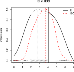
The right-hand panels in Figure 3 show a similar sequence of plots in the presence of a known constraint . To illustrate EI and IECI in this scenario, consider the random realization and corresponding posterior predictive surface in the top-right panel. Here the design locations all reside inside . The bottom-right panel shows the EI statistic over the entire (discrete) range for , as above. Those parts of the EI curve corresponding to inputs which violate the constraint are dotted. The EI is maximized outside of the constraint region near , with the maximal value inside at the boundary. The IECI statistic is also shown over the entire range, but the locations are restricted to . I.e., . This is so that we may consider the extent to which every location reduces the average conditional improvement . Observe that the maximal IECI point is . This point gives the greatest reduction in improvement averaged over the constraint region, even though it does not, itself, satisfy the constraint.
4 Dealing with Unknown Constraints
Here we extend the IECI to unknown constraints. Much of the necessary scaffolding has already been built into the IECI via , e.g., . It remains for us to flesh out the Monte Carlo by incorporating the surrogate for . We extend the parameter vector to contain parameters for both surrogates: ; and the data to include the class/constraint labels: . Inference for unknown is via samples from the joint posterior. An appropriate choice of is discussed in Section 4.1.
For now, overload the generic classification surrogate notation to let denote the probability input satisfies the constraint given parameters . Then,
| (14) |
Note that in there is an implicit dependence upon , unless these parameters are taken as known. In that case we may drop the superscript from the ECI expression in Eq. (14), and re-arrange the order of summation to avoid unnecessarily re-calculating the ECI for each . Observe that Eq. (14) extends Eq. (13) rather than (12). Sampling from the surrogate , rather than simply evaluating the related quantity , would not generally be straightforward, and so we prefer to work with design-based candidates .
4.1 An Appropriate Constraint Surrogate, and Sequential Inference
An appropriate partner to the canonical GP (regression) surrogate for is a classification GP (CGP) surrogate for . For details on CGP specification and corresponding Monte Carlo inference based on MCMC, see Neal, (1998). As in the regression case, the CGP model is highly flexible and competitive with, or better than, the most modern models for non-parametric classification. However, batch inference methods based on MCMC are at odds with the sequential nature of the design strategy. Except to guide the initialization of the new Markov chain, it is not clear how fits from earlier iterations may re-used in search of the next design point. So after each sequential design step the MCMC must be re-started and iterated until convergence. The result is a slow algorithm.
So instead of taking the traditional, established, MCMC approach to C/GP inference we follow a new sequential Monte Carlo (SMC) approach outlined by Gramacy and Polson, (2010). They show how GP and CGP models can be implemented in an online setting, by quickly updating a discrete approximation to the posterior via particle learning (Carvalho et al.,, 2008). This approach leads to fast online—and in some cases statistically superior (i.e., lower MC error)—posterior summaries compared to MCMC. Gramacy and Polson, (2010) go on to describe to how EI for optimization and entropy based boundary exploration for classification can proceed efficiently with particles. This is easy to extend to IECI by coupling the regression and classification models ( and ) via the Monte Carlo approximations described earlier in this paper.
4.2 Illustrations and Examples
We provide two synthetic data examples where the constraint region is unknown. In both cases we take the candidate and reference locations (identically: ) as a LHD randomly generated at the beginning of each round and then augmented with an oracle point (Taddy et al.,, 2009b). We follow Gramacy and Taddy, (2010) in taking the oracle point as the local maximum obtained via numerical non-derivative minimization initialized at the last added design point and searched over the MAP predictive surface inferred in the previous round. An implementation via particles is described by (Gramacy and Polson,, 2010).
The objective function and constraint region for the first example was presented in Section 3.3. We initialize the optimization with a size 20 LHD, and then collect 60 points by IECI with 100 fresh candidates/reference locations as described above.
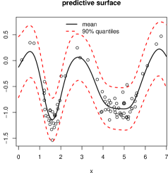
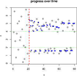

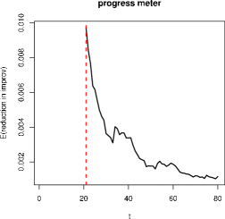
Figure 4 summarizes the results after the 80 total samples were gathered. Observe from the plots in the top row that most samples (after the 20 initial ones) were gathered in the two local minima, with a few taken outside . The oracle candidates (solid circles) indicate the most likely locations of minima according to the posterior predictive distribution. The bottom panes show an estimate of via the posterior mean probability of violating the constraint (), and a progress meter showing the largest (log) expected reduction in average improvement (7) at each round. Observe how the ability to improve upon the current minimum decreases over time, giving a heuristic indication of convergence.
In our second example, the objective function for 2-d inputs is given by
| (15) | ||||
and observed without noise. The constraint (satisfaction) region is the interior of an ellipse defined by the 95% contour of a bivariate normal distribution centered at the origin, with correlation and variance . The true global minimum is at , which does not satisfy the constraint. There are, however, three other local minima—two of which satisfy the constraint. The setup is as described above for the 1-d example except that the optimization is initialized with 25 LHD samples, after which 100 are gathered by IECI with 100 fresh candidates in each round.
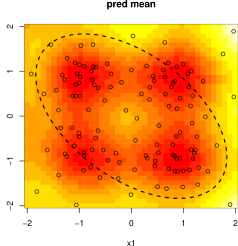
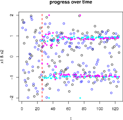
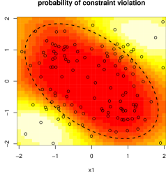
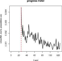
Figure 5 summarizes the results after the 125 total samples were gathered. Observe that very few samples were gathered outside the unknown constraint region, except near the local minima. It is sensible to sample heavily on the boundary of the constraint region where the response is quickly changing and local minima are likely to occur. This is in case the global minimum is on the boundary, and also helps to extract the GP parameters in regions of highest importance. Notice that large concentrations of samples occur for the two minima well inside the constraint region. But the bottom-right plot indicates that further progress can be made by additional sampling.
5 Health Policy Optimization
Our motivating example involves a simulation of health care policy in the United States. The COMPARE simulator (Girosi et al.,, 2009) was developed at the RAND Corporation to predict the effect of various health care policies in terms of individual choices of health insurance and the associated costs. It is an agent-based microsimulation model that uses a maximum utility approach to predict the health insurance decisions of individuals, families, and firms as a function of a wide range of inputs on available types of policies, and on taxes, penalties, and regulations. The population is simulated based on Census Bureau data. Additional datasets provide values for many of the parameters in the simulation, and other parameters are set as part of the possible policy interventions. However, there are several calibration parameters that are tuned so that when the simulator is run on current policies, it makes predictions as close as possible to the current observable situation in the United States. Such a calibration can be viewed as a minimization problem, choosing the values of the calibration parameters to minimize the discrepancy between predictions and reality. This setup is common for computer simulators and has been investigated in the unconstrained setting (e.g., Kennedy and O’Hagan,, 2001). What differs from the standard setup here is the presence of unknown constraints.
The simulator has a number of inputs and outputs, here we focus on a subset deemed most important by our collaborators, the designers of the simulator. The inputs over which we optimize are a set of six calibration parameters: utility tuning parameters for adults on ESI programs, adults on individual programs, and adults on public programs, and an analogous set of three parameters for children. The outputs of interest are the predicted counts in each type of insurance (or the uninsured category) and the elasticities of response for the key categories of adults in individual plans, adults in restricted individual plans, uninsured adults, children in individual plans, children in restricted individual plans, and uninsured children. The objective function specified by our collaborators is a combination of the absolute errors in the predicted counts and the squares of the predicted elasticities:
where , , and are constants specified by our collaborators that weight the pieces appropriately. Our goal is to minimize this objective function under the constraint that the elasticities for the insured are negative and the elasticities for the uninsured are positive. The elasticities can only be found by running the simulator, so this set of constraints fits under our unknown constraints regime.
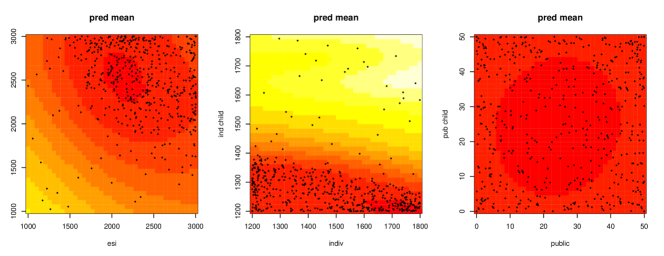
Figure 6 shows pairwise slices of the fitted response surface. The left panel shows how the fitted predicted surface varies as a function of the parameters for adult and child ESI, when the other four parameters are held fixed at a value around that which produces the minimum response. The middle and right panels vary by the parameters for individual programs and public programs respectively. Dark shades are lower values, so it can be seen that both ESI parameters need to be relatively high, the child individual parameter needs to be low, and the other three parameters are relatively less important. The points plotted in the figure are the 550 total inputs sampled projected into the each of the three pairs of input coordinates.
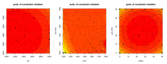
Figure 7 shows the fitted probability of a constraint violation over the portions of the space which were routinely sampled. As seen in Figure 6, some regions are not well-sampled because they do not help in finding the minimum, the goal of the problem. These sparsely sampled regions do not provide much information for estimating the probability of a constraint violation (which is not the primary goal of the problem), and so the estimated values are overly influenced by the prior mean. Thus we only display parts of the regions in the first two plots to better show the estimated probabilities. Sampled points which violated the constraints are shown with asterisks. One can see that the largest probabilities of constraint violations occurred for large values of the ESI parameter, for jointly small values of the individual and child individual parameters, and for values of the public and child public parameters which are in the corners of the space.
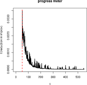
Figure 8 shows the progress meter (7) over the 500 optimization rounds which can be used as a heuristic check of convergence. As in previous examples, the noisiness in the meter is due to the LHD predictive grid of 100 candidates at which the IECI is evaluated in each round. After about 250 samples the IECI seems to have “bottomed-out”. However, further progress can be made to reduce the frequency and magnitude of the “up-spikes” in the remaining optimization rounds, and thereby obtain higher confidence that the constrained global minimum has been obtained.
6 Discussion
We have introduced a statistical approach to optimization under unknown constraints by an integrated conditional expected improvement (IECI) statistic. The idea is to consider how the improvement at reference locations () conditional on candidates () may be used to augment a design. Without considering constraints, the resulting statistic is a less greedy—aggregated—version of the standard expected improvement (EI) statistic. Another way to obtain a less greedy EI is to raise the improvement to a power (Schonlau et al.,, 1998). The IECI approach, by contrast, does not require such a tuning parameter. In the presence of unknown constraints, IECI allows us to coherently consider how design candidates adjust the improvement at reference locations believed to satisfy the constraint. Our method was illustrated on two synthetic examples and a motivating problem from health care policy. An implementation is provided in the plgp package on CRAN.
We envisage many ways that our methodology may be extended and improved. Understanding of convergence of statistical optimization algorithms is scant at best, and IECI is no exception. While we provide a sensible heuristic that seems to work well in our examples, much remains to be done in this area. It may also be sensible to model the constraint as a function of the inputs () and the real-valued response (). An example of where this would be handy is when , for some constant . Our dual-GP modeling framework may easily be extended to allow uncertainty in (real-valued) responses to filter through, as predictors, into the surrogate model for the classification labels. A more difficult extension involves accommodating hidden constraints (Lee et al.,, 2010): where evaluation of the real-valued response fails, e.g., due to a lack of convergence in a simulation. Finally, it may be worthwhile to consider surrogate models beyond GPs. Dynamic trees for regression and classification show considerable promise (Taddy et al.,, 2010).
Acknowledgments
This research was initiated at a workshop at the American Institute of Mathematics (AIM) on Derivative-Free Hybrid Optimization Methods for Solving Simulation-Based Problems in Hydrology, and was also partially supported by NSF grant DMS-0906720 to HKHL and EPSRC grant EP/D065704/1 to RBG. The authors would like thank Crystal Linkletter for interesting discussions at AIM, the RAND Corporation, Health division, for the use of COMPARE, and Federico Girosi, Amado Cordova, and Jeffrey Sullivan in particular for their help with the simulator.
References
- Abrahamsen, (1997) Abrahamsen, P. (1997). “A Review of Gaussian Random Fields and Correlation Functions.” Tech. Rep. 917, Norwegian Computing Center, Box 114 Blindern, N-0314 Oslo, Norway.
- Carvalho et al., (2008) Carvalho, C., Johannes, M., Lopes, H., and Polson, N. (2008). “Particle Learning and Smoothing.” Discussion Paper 2008-32, Duke University Dept. of Statistical Science.
- Girosi et al., (2009) Girosi, F., Cordova, A., Eibner, C., Gresenz, C. R., Keeler, E., Ringel, J., Sullivan, J., Bertko, J., Buntin, M. B., and Vardavas, R. (2009). “Overview of the COMPARE Microsimulation Model.” Tech. Rep. WR-650, RAND.
- Gramacy and Polson, (2010) Gramacy, R. and Polson, N. (2010). “Particle learning of Gaussian process models for sequential design and optimization.” Tech. Rep. arXiv:0909.5262, University of Cambridge.
- Gramacy, (2005) Gramacy, R. B. (2005). “Bayesian Treed Gaussian Process Models.” Ph.D. thesis, University of California, Santa Cruz.
- Gramacy and Lee, (2008) Gramacy, R. B. and Lee, H. K. H. (2008). “Bayesian treed Gaussian process models with an application to computer modeling.” Journal of the American Statistical Association, 103, 1119–1130.
- Gramacy and Lee, (2009) — (2009). “Adaptive Design and Analysis of Supercomputer Experiment.” Technometrics, 51, 2, 130–145.
- Gramacy and Taddy, (2010) Gramacy, R. B. and Taddy, M. A. (2010). “Categorical Inputs, Sensitivity Analysis, Optimization and Importance Tempering with tgp Version 2, an R Package for Treed Gaussian Process Models.” Journal of Statistical Software, 33, 6, 1–48.
- Jones et al., (1998) Jones, D., Schonlau, M., and Welch, W. J. (1998). “Efficient Global Optimization of Expensive Black Box Functions.” Journal of Global Optimization, 13, 455–492.
- Kennedy and O’Hagan, (2001) Kennedy, M. and O’Hagan, A. (2001). “Bayesian Calibration of Computer Models (with discussion).” Journal of the Royal Statistical Society, Series B, 63, 425–464.
- Lee et al., (2010) Lee, H., Gramacy, R., Linkletter, C., and Gray, G. (2010). “Optimization Subject to Hidden Constraints via Statistical Emulation.” Tech. Rep. UCSC-SOE-10-10, University of California, Santa Cruz, Department of Applied Mathematics and Statistics.
- Neal, (1998) Neal, R. M. (1998). “Regression and classification using Gaussian process priors (with discussion).” In Bayesian Statistics 6, ed. e. a. J. M. Bernardo, 476–501. Oxford University Press.
- O’Hagan et al., (1999) O’Hagan, A., Kennedy, M. C., and Oakley, J. E. (1999). “Uncertainty Analysis and Other Inference Tools for Complex Computer Codes.” In Bayesian Statistics 6, eds. J. M. Bernardo, J. O. Berger, A. Dawid, and A. Smith, 503–524. Oxford University Press.
- Sacks et al., (1989) Sacks, J., Welch, W. J., Mitchell, T. J., and Wynn, H. P. (1989). “Design and Analysis of Computer Experiments.” Statistical Science, 4, 409–435.
- Santner et al., (2003) Santner, T. J., Williams, B. J., and Notz, W. I. (2003). The Design and Analysis of Computer Experiments. New York, NY: Springer-Verlag.
- Schonlau et al., (1998) Schonlau, M., Jones, D., and Welch, W. (1998). “Global versus local search in constrained optimization of computer models.” In New Developments and applications in experimental design, no. 34 in IMS Lecture Notes - Monograph Series, 11–25. Institute of Mathematical Statistics.
- Seo et al., (2000) Seo, S., Wallat, M., Graepel, T., and Obermayer, K. (2000). “Gaussian Process Regression: Active Data Selection and Test Point Rejection.” In Proceedings of the International Joint Conference on Neural Networks, vol. III, 241–246. IEEE.
- Taddy et al., (2010) Taddy, M., Gramacy, R., and Polson, N. (2010). “Dynamic trees for learning and design.” Tech. Rep. arXiv:0912.1636, University of Chicago.
- Taddy et al., (2009b) Taddy, M., Lee, H. K. H., Gray, G. A., and Griffin, J. D. (2009b). “Bayesian Guided Pattern Search for Robust Local Optimization.” Technometrics, 51, 389–401.
- Gramacy, (2010) — (2010). plgp: Particle Learning of Gaussian Processes. R package version 1.0.