Hashing Image Patches for Zooming
Abstract
In this paper we present a Bayesian image zooming/super-resolution algorithm based on a patch based representation. We work on a patch based model with overlap and employ a Locally Linear Embedding (LLE) based approach as our data fidelity term in the Bayesian inference. The image prior imposes continuity constraints across the overlapping patches. We apply an error back-projection technique, with an approximate cross bilateral filter. The problem of nearest neighbor search is handled by a variant of the locality sensitive hashing (LSH) scheme. The novelty of our work lies in the speed up achieved by the hashing scheme and the robustness and inherent modularity and parallel structure achieved by the LLE setup. The ill-posedness of the image reconstruction problem is handled by the introduction of regularization priors which encode the knowledge present in vast collections of natural images. We present comparative results for both run-time as well as visual image quality based measurements.
1 Introduction
Inferring a high resolution image from a single or a given set of spatially coherent low resolution images has been a problem which has been studied by numerous researchers in the past. Different algorithms have been proposed to this end which find implementations in the real world to handle different scenarios as well as end goals. For instance, super-resolution of faces has an entirely different set of literature which takes help from the vast field of face identification and detection, whereas, super-resolution of natural images still remains in the domains of interpolation and optimization techniques. Simple applications like increasing the size of a digital image to complex scenarios like identifying suspects from a surveillance video can all be modeled as some form of super-resolution problem. Most of the techniques proposed till now can be broadly classified into two main categories. Iterative time/frequency domain methods and learning based techniques. Iterative techniques can be traced back to the seminal work by Tsai and Huang [9], which was then modified to the first iterative implementation by Irani et. al. [11]. Iterative methods use a Bayesian framework wherein an initial guess about the high resolution frame is refined at each iteration. The image prior is usually assumed to be a smoothness prior. Iterative methods are inherently context independent and hence a few problems encountered in cases like eyes in face enhancement still remain tough problems for the iterative methods. Geman and Geman [6], introduced an optimization framework wherein a compatibility model of high-resolution to low-resolution image features is constructed, and then the inverse reconstruction problem can be solved by searching in the compatibility space. Their work proposed modeling the unknown image as a Markov Random Field (MRF) where neighboring image regions are assumed to be Markovian in nature, thereby simplifying the inference problem. Given enough training data, searching through compatibility space techniques have been shown to work wonderfully well. Freeman et al [5], studied natural image super-resolution using Belief Propagation (BP) algorithm [16] for inference in MRFs. The results clearly show the superiority of the proposed method, but the run time for the algorithm remained a bottleneck for the practical implementation of their algorithm.
Another interesting approach was proposed by Chang et. al. [2], wherein they posed learning based super-resolution as locally linear manifold estimation problem based on the work by Roweis et al. [18]. Their method was based on the fact that low-resolution image patches can be represented by linear combinations of a few local patches which are the nearest neighbors of the test patch in the low-resolution training set. Corresponding high-resolution patches are then linearly combined and the high-resolution patch is thereby inferred. The convex set of coefficients learned for the low-resolution space are translated as is to the high-resolution space. Boundary issues were handled by simple averaging over pixel values. Example based super-resolution methods have a similar flavor to the region growing based texture synthesis technique proposed by Efros and Leung [4]. Texture synthesis can be assumed to be a sub-problem to generic super-resolution, which tries to exploit the regularities present in pure textures, wherein a candidate region is grown based on sampling from the space of the nearest neighbors. This works efficiently for pure textures, but when the scene consists of greater details than one uniform texture, which is characterized by an inherent sense of repeatability, then the manifold based technique produces much better results. A similar method has been proposed for face enhancement, commonly known as hallucination, by Park et. al. [15] wherein they propose linearity preserving projections. Manifold based techniques have also been used for successful image retrieval as investigated by He et. al. [8]. But for most of these methods the nearest-neighbor search still presents a bottleneck for practical implementations.
In recent years, several researchers proposed to avoid the running time bottleneck by using approximation techniques [1, 10, 7]. Locality Sensitive Hashing (LSH), which tries to address a similar problem was proposed by Indyk et. al. [10]. The key idea is to hash the points using several hash functions so as to ensure that, for each function, the probability of collision is much higher for objects which are close to each other than for those which are far apart. One can determine near neighbors by hashing the query point and retrieving elements stored in buckets containing that point. The algorithm proposed in [7] worked in the hamming space and such it assumed the data points to be in space. In this work we extend the work of Datar et. al. [3]. Their work introduced the idea of p-stable distributions to generate the hash functions and showed that this technique can be implemented directly on the data space without transformation to the hamming space.
2 Motivation
In this paper we present a method which builds on the algorithm proposed by Chang et. al. [2], with a few key differences which render this work unique and the first of its kind to the best of our knowledge. The nearest neighbor estimation step mentioned in the original work by Roweis et. al. [18], has been used as is in the work by Chang et. al. [2]. This technique presents the most crucial bottleneck in the scalability as well practical use of their algorithm. We counter this deficiency by employing Locality Sensitive Hashing scheme which works well in scenarios where nearest neighbor (NN) problem can be approximated by an -NN problem [3], defined later in Sec 3.2. For the method proposed by Chang et. al. [2], the image reconstruction quality quickly deteriorates due to the lack of effective regularization. We counter this by a back-propagation technique, where we introduce an optimized approximation of the bilateral filter which has been shown to preserve edges while simultaneously suppressing noise.
The rest of the paper is organized as follows. We introduce the notations in Sec 2.1 which would be consistently used for the rest of this paper. In Sec 3.1, Sec 3.2 and Sec 3.3 we introduce the mathematical details for the three main techniques which form the crux of our work. Sec 4, illustrates the main body of this work. We enlist the modifications and enhancements made to each of the techniques mentioned earlier, to make them work for our application. We present the experimental details in Sec 5. Finally, we conclude our work with discussions about ongoing and future work in Sec 6.
2.1 Notations
Let denote the set of high-resolution images, from which we generate the corresponding set of low-resolution images by first blurring by a Gaussian kernel , where denotes the spread of the kernel, and then down-sampling by a factor , when not specified explicitly. The low-resolution images are then interpolated back to the original size of the high-resolution images, so that corresponding images are of the same size. Individual low and high resolution image pairs are then divided into overlapping patches denoted by , , where denotes the image index, and denotes the patches in the low/high image pair in the training data. We will drop the image index in the later sections when it is clear that only patch index is required to identify the low/high resolution patch pairs. The patches are numbered in row-principle order for each image. Note, that the patch index runs through all the images in the training set assigning unique integer ID’s to each patch from each image in the training data. The notation specifically denotes the total number of patches generated for the entire data set. Also note that there are high resolution patches and low-resolution patches which need to be explicitly stored onto the disk.
3 Background
3.1 Locally Linear Embedding (LLE)
LLE as a manifold learning technique was introduced by Roweis et. al. [18], wherein they proposed a local neighborhood based linear estimation technique to unfold complex manifolds. The key idea is to compute locally linear weights to approximate the actual high-dimensional space. This method has found many applications in the fields of machine learning and computer vision, and Chang et. al. [2] were one of the first group of researchers to propose an LLE based algorithm for image super-resolution.
Suppose there are points in a high-dimensional space of dimension . The points are assumed to lie on a manifold of dimension , where . The principle assumption of this technique is that if the manifold is smooth, meaning the local changes in the topology can be assumed to be linear, then a sample on the manifold can be approximated by a linear combination of a few of its neighbors. As such the two main components of the LLE algorithm are
-
1.
For each data point in the D-dimensional data space:
-
(a)
Find the set of nearest neighbors in the same space.
-
(b)
Compute the reconstruction weights of the neighbors that minimize the reconstruction error.
-
(a)
-
2.
Compute the low-dimensional embedding in the dimensional embedding space such that it best preserves the local geometry represented by the reconstruction weights.
3.2 Locality Sensitive Hashing (LSH)
Nearest neighbor problem can be relaxed by posing it as an -NN problem, where the aim is to return a point which is at a distance from the query point , when there is a point in the data set within distance from . LSH technique was introduced by Indyk et. al. [10], to solve the -NN problem . For a domain of the points set with distance measure , an LSH family is defined as:
Definition 1
A family is called sensitive for if for any ,
where is the ball of radius centered at and .
such hash functions are concatenated to form a new function class such that , where . such functions are chosen independently uniformly at random and form the buckets into which the training patches are hashed. During testing the test patches are hashed into the buckets and all the matching training patches are extracted as the nearest neighbors.
3.3 Bilateral filter
Bilateral filtering [19], is a non-linear filtering technique which combines image information from spatial domain as well as the feature domain. It can be represented by the following equation
| (1) |
where and are the input and the output images respectively, and are pixel locations, and is the neighborhood around the pixel .
| (2) |
is a normalization term at pixel . Normally the function is defined as
| (3) |
and similarly the filter is defined as
| (4) |
4 Bayesian Inference with back-propagation
Denote the input low resolution (LR) image as and the true high resolution (HR) image as . Now we can write
| (5) |
The maximum likelihood estimate then gives an estimate for the best . the error image which is the deviation from the current inference to the observed image is then computed as
| (6) |
Here is a smoothing kernel and represents the convolution in spatial domain. Back-propagation technique, introduced by Irani et. al. [11], adds a smoothed version of the error image to the current estimate of the HR image.
| (7) |
is the back-projection filter and can be similar to . We substitute a bilateral filter kernel for the back-projection filter as mentioned in the forthcoming sections.
For a patch based representation, assuming Gaussian noise model, the negative log likelihood term can be written as
| (8) |
where is the total number of patches of size in the image and is a metric discussed in detail in the later sections. We also assume that the sample rate discrepancies have been absorbed into . The image prior is assumed to be a smoothness constraint imposed on the overlapping boundary of the patches. For two neighboring patches in the HR image the image prior is denoted as
| (9) |
Now let us look at the likelihood term in greater detail. For each patch in the LR image, we find the closest patches in the LR dataset and compute the LLE reconstruction weights. Then, we impose the same reconstruction weights on the corresponding HR patches and reconstruct the HR patch. The search in the LR space is usually the speed bottleneck for such methods. We implement a variant of the LSH technique to alleviate this problem.
4.1 Hashing
Datar et. al. [3], showed that Gaussian distribution is a p-stable distribution under norm, and hence preserved distances after projection by a Gaussian random vector. It has been proved that projection by Cauchy random vectors preserve distances [21]. Recent research work on the statistics of natural images [13, 20], has shown that natural images have sparse derivatives, which follow an approximate Laplacian distribution. This hints at an type of distance metric for the nearest neighbor searching. Based on this knowledge we chose the following formulation for our hash function
| (10) |
where is an integer chosen to balance the hash bins, is a uniform random number chosen from and is a Cauchy random vector whose elements are sampled from the rule
| (11) |
where represents a normal distribution. is some feature representation of a low-resolution patch and denotes the integer less than or equal to . We concatenate such hash functions and form hash table. Based on the integers we form the bins in the table and store the integer ID corresponding to the patch into the hash table. such hash tables are formed for matching the test patches against the training patches. We introduce a hash match criterion during matching which states that a matching patch ID found in one hash table should be present in at least out of hash tables.
Feature representation: The low-resolution patches are represented as gradient based features for hashing. We use different feature representations ranging from first order gradient (convolution with [], ) to second order gradient (convolution with [], ).
Hashing Quality (determining ): Entropy has been one of the most widely accepted metrics for measuring the quality of hashing. In our case entropy directly translates to the speed of generating the list of all the approximate nearest neighbors. But improving the entropy can sometimes lead to poor image reconstruction quality, which hints at a tradeoff for practical implementations. The denominator in Eqn 10, is used to control the quality of hashing,
4.2 Locally Linear Embedding
Let us denote the test patch as . We query for the test patch into each hash table and collect all the matches found, where . We purposefully drop the image index as introduced in Sec 2.1, because after the training stage all patches are treated equally, independent of their originating images. If is larger than some pre-defined number of matches (typically ) further searching is stopped. Once the matches have been identified, we solve the following constrained least square minimization problem
| (12) | |||||
| (13) |
Once, the weight matrix is computed the high-resolution patch corresponding to can simply be written as
| (14) |
For, all the results shown later in the paper, we have used patches with one pixel width overlap. Going back to the metric introduced in Eqn. 8, the metric is equivalent to solving the LLE reconstruction equation in Eqn. 12, based on the neighbors found by the hashing scheme.
4.3 Approximate Bilateral Error Propagation
Normally, the filter is defined as in Eqn. 4. But in this paper, we present a different formulation for this filter. The main concern with numerous researchers with the simple form of bilateral filter is the fact that, the complexity of the filter grows as . In view of the kernel size bottleneck, we define the filter as
| (15) |
where the notation just denotes the cardinality of the neighborhood We also borrow from Paris et. al. [14], and adopt the idea of cross bilateral filtering wherein, and can come from different images. Since this filter operates on the error image, we replace terms with , where represents the error between the original LR image and bi-cubic interpolated HR image. The new formulation of the range filter can now be exploited, since the mean over the filter kernel, can be computed extremely efficiently. Again, borrowing from Porikli [17], we adopt the integral image technique, which renders the evaluation of the filter in Eqn. 4, an operation. The new filter can now be written as
| (16) |
Assuming a normalized filter , and denoting the filter response for for the entire image as , we can write the filter response succinctly as
| (17) |
where means an elementwise multiplication.
5 Experiments and Results
5.1 Training Data Generation
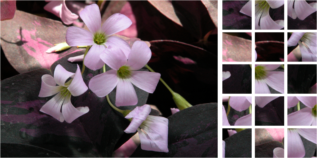
One of the key benefits of our method over others is the fact that it can handle relatively large amounts of training data. Because of the approximate nearest neighbor search, facilitated by the LSH formulation, the inference algorithm only looks at a sub-part of the training data. To generate the training data for the experiments shown in Fig 4, we collected high resolution images from [12]. We compute the horizontal and vertical first order gradient at each pixel location of an image and then generated a cumulative distribution function based on the gradient values. We sampled for the center pixel location and then saved a image centered at this pixel. such samples were drawn at random from each of the images chosen form [12] and then saved as training images. Each training image is then blurred and downsampled to form the low-resolution counterpart for the high resolution training images. For a patch size of , with an overlap of 2 pixels, we collect a total of around patch pairs from one image. The total number of training patch pairs is of the order of patch pairs. Examples of the sub-images collected from one image is shown in Fig 1. For all the results none of the test images were present in the training set. For Fig 2, we added a small part of the image in the training set.
5.2 Comparative Results
We present the comparative results for our algorithm against standard image interpolation techniques like bicubic interpolation. We also compare our results against similar learning based techniques like Chang et. al. [2] and Freeman’s method [5]. We present comparative run-time analysis against Chang [2], where we count one nearest neighbor as one operation. Our analysis clearly proves the time efficiency achieved by incorporating the hashing scheme into the linear embedding technique used in [2].
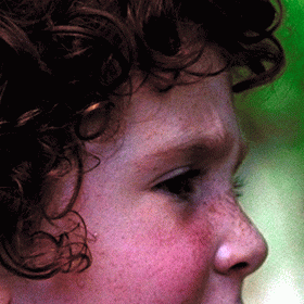
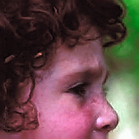
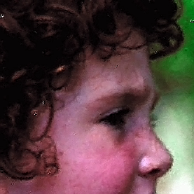
The first set of results were performed on the little girl image which was presented in [5] and has since been used by numerous researchers for comparison. Fig 2 presents the comparative results of our method against [5]. Note that Fig 2(c) has been taken from the author’s website111http://www.ai.mit.edu/people/wtf/superres. One primary benefit of our method over [5] is the fact that our method goes through all the patches in the test image just once, compared to an iterative belief propagation routine in [5], and hence can handle large amount of training data, while still being able to generate acceptable results. 40,000 training patch pairs were reported in [5] and they run the process for upto 10 iterations. The run time for their method on our system (Pentium 4, 3Mhz, 2MB RAM) was of the order of 6 minutes for one iteration, which results to around 60 minutes runtime for an image which is of size . Our method runs in one iteration and takes around 1 minute for generating the results. Note that our training set for this experiment contained around 300,000 patch pairs, which is roughly 3 times that handled by [5].
We compare our run times against Chang et. al. [2] as presented in Fig 3. As hinted earlier, we denote each similarity against a patch in the training data base as one time unit and count the number of similarity checks we need to perform to generate the results. Since comparing against the training patches is the most important part of the algorithm (and also the most time consuming one), this can be treated as a fair comparison for the run times of the two algorithms. We compute mean number of similar patches generated by our algorithm to infer all the patches of the test image. For [2] this number remains fixed at the total number of patches in the training set.

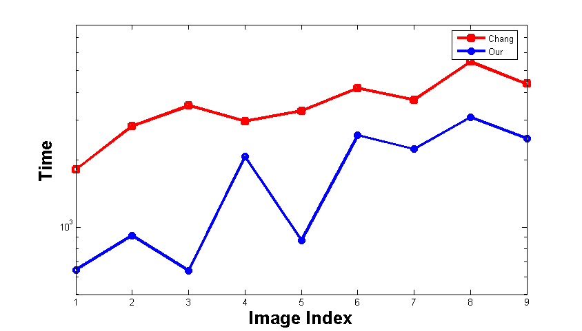
Fig 3 (top) shows the MSE for different experiments averaged times each. The two curves are almost similar strengthening our claim that the approximate nearest neighbor hashing scheme performs almost at par with the complete nearest neighbor scheme. On average we underperform by a factor of about (for images which are all larger than pixels)which is negligible compared to the time gain which we accomplish by our method. Fig 3 (bottom) shows the comparison of the quality factor for the two methods. Note that the quality comparison results are shown in log scale to reduce the wide gain achieved by our method over Chang’s [2] method, and plot both the curves in the same figure. As mentioned earlier, we learn hash tables and hence deal with times the training data, but still manage to generate improvements in run time by orders of magnitude. The maximum improvement in runtime is around 2 on the log scale which is about 100 times. The average time gain is about 70 times over Chang’s [2] method. The run times reported in this paper are all generated on a single machine. The structure of the algorithm can be exploited to break the problem into similar sub-problems and can be run on different machines.
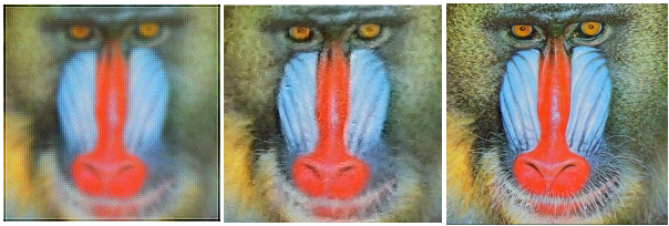
Next set of results compare our method against bicubic interpolation as shown in Fig 4. Since, bicubic interpolation by itself cannot match our results, we perform an additional unsharp operation and report the comparative results in Fig 4. We also perform similar experiments for de-blurring and zooming. Fig 5 shows input blurred image and the result of our algorithm along with the original HR image. Fig 6 shows the input image stretched two times and the result of our algorithm along with the original HR image.




6 Conclusion and Future work
In this paper we present a truly large scale system able to handle large amounts of data in acceptable time for image zoomiong/super-resolution. We introduce the idea of LSH for feature based image patch hashing for efficient approximate nearest neighbor identification in close to constant time. An LLE based scheme, is then employed to infer the high-resolution patches. We present image reconstruction results as well as run-time comparisons against established learning based methods.
References
- [1] S. Arya, D. Mount, N. Netanyahu, R. Silverman, and A. Wu. An optimal algorithm for approximate nearest neighbor searching. In Proc. Fifth Annual ACM-SIAM Symposium on Discrete Algorithms, pages 573–582, 1994.
- [2] H. Chang, D. Y. Yeung, and Y. Xiong. Super-resolution through neighbor embedding. In Proc. of IEEE Conf. on Computer Vision and Pattern Recognition (CVPR), volume 1, pages 275–282, 2004.
- [3] M. Datar, N. Immorlica, P. Indyk, and V. S. Mirrokni. Locality-sensitive hashing scheme based on p-stable distributions. In SCG ’04: Proc. of the twentieth annual symposium on Computational geometry, pages 253–262, New York, NY, USA, 2004. ACM.
- [4] A. A. Efros and T. K. Leung. Texture synthesis by non-parametric sampling. In IEEE International Conference on Computer Vision, pages 1033–1038, Corfu, Greece, September 1999.
- [5] W. T. Freeman, E. C. Pasztor, and O. T. Carmichael. Learning low-level vision. International Journal of Computer Vision, 40(1):25–47, 2000.
- [6] S. Geman and D. Geman. Stochastic relaxation, gibbs distributions, and the bayesian restoration of images. In IEEE Trans. on Patten Analysis and Machine Intelligence, volume 6, pages 721–741, 1984.
- [7] A. Gionis, P. Indyk, and R. Motwani. Similarity search in high dimensions via hashing. In Proc. 25th International Conference on Very Large Data Bases (VLDB), 1999.
- [8] X. He, W.-Y. Ma, and H.-J. Zhang. Learning an image manifold for retrieval. In MULTIMEDIA ’04: Proceedings of the 12th annual ACM international conference on Multimedia, pages 17–23, New York, NY, USA, 2004. ACM.
- [9] T. S. Huang and R. Tsai. Multi-frame image restoration and registration. In T. S. Huang, editor, Proc. Advances in Computer Vision and Image Processing, volume 1, pages 317–339. JAI Press Inc., 1984.
- [10] P. Indyk and R. Motwani. Approximate nearest neighbor: towards removing the curse of dimensionality. In Proc. Symposium on Theory of Computing, 1998.
- [11] M. Irani and S. Peleg. Improving resolution by image restoration. In CVGIP: Graph. Models Image Processing, volume 53, pages 231–239, 1991.
- [12] A. Olmos and F. A. A. Kingdom. (2004) McGill Calibrated Colour Image Database, http://tabby.vision.mcgill.ca.
- [13] B. Olshausen and D. J. Field. Emergence of simple cell receptive field properties by learning a sparse code for natural images. Nature, 381:607 608, 1996.
- [14] S. Paris and F. Durand. A fast approximation of the bilateral filter using a signal processing approach. International Journal of Computer Vision, 2009.
- [15] J. S. Park, J. Lee, and S. W. Lee. Region-based reconstruction for face hallucination. In Advances in Multimedia Modeling, 13th International Multimedia Modeling Conference, MMM 2007, volume 4351, pages 44–53. Springer, Jan 2007.
- [16] J. Pearl. Probabilistic reasoning in intelligent systems: networks of plausible inference. Morgan Kaufmann Publishers Inc., 1988.
- [17] F. Porikli. Constant time O(1) bilateral filtering. In Proc. of Compuetr Vision and Pattern Recognition, CVPR08, pages 1–8, 2008.
- [18] S. Roweis and L. Saul. Nonlinear dimensionality reduction by locally linear embedding. In Science, volume 290, pages 2323–2326, Dec 2000.
- [19] C. Tomasi and R. Manduchi. Bilateral filtering for gray and color images. In Proc. of International Conference of computer Vision, ICCV98, pages 839–846, 1998.
- [20] Y. Weiss. Deriving intrinsic images from image sequences. In Proc. Eighth IEEE International Conference on Computer Vision ICCV, volume 2, pages 68–75, 2001.
- [21] V. Zolotarev. One-dimensional stable distributions. In Translations of Mathematical Monographs, volume 65. American Mathematical Society, 1986.

