Systematic Effects on Determination of the Growth Factor
from Redshift-space Distortions

Abstract

The linear growth factor of density perturbations is generally believed to be a powerful observable quantity of future large redshift surveys to probe physical properties of dark energy and to distinguish among various gravity theories. We investigate systematic effects on determination of the linear growth factor $f$ from a measurement of redshift-space distortions. Using a large set of high-resolution $N$-body simulations, we identify dark matter halos over a broad mass range. We compute the power spectra and correlation functions for the halos and then investigate how well the redshift distortion parameter $\beta\equiv f/b$ can be reconstructed as a function of halo mass both in Fourier and in configuration space, where $b$ is the bias parameter. We find that the $\beta$ value thus measured for a fixed halo mass generally is a function of scale for $k>0.02{\hbox{$~{}h{\rm~{}Mpc}^{-1}$}}$ in Fourier space or $r<80{\hbox{$~{}h^{-1}$}{\rm~{}Mpc}}$ in configuration space, in contrast with the common expectation that $\beta$ approaches a constant described by Kaiser’s formula on the large scales. The scale dependence depends on the halo mass, being stronger for smaller halos. It is complex and cannot be easily explained with the exponential distribution function in configuration space or with the Lorentz function in Fourier space of the halo peculiar velocities. We demonstrate that the biasing for smaller halos has larger nonlinearity and stochasticity, thus the linear bias assumption adopted in Kaiser’s derivation become worse for smaller halos. Only for massive halos with the bias parameter $b\geq 1.5$, the $\beta$ value approaches the constant predicted by the linear theory on scales of $k<0.08{\hbox{$~{}h{\rm~{}Mpc}^{-1}$}}$ or $r>30{\hbox{$~{}h^{-1}$}{\rm~{}Mpc}}$. Luminous red galaxies (LRGs), targeted by the Sloan Digital Sky Survey (SDSS) and the SDSS-III’s Baryon Oscillation Spectroscopic Survey (BOSS), tend to reside in very massive halos. Our results indicate that if the central LRG sample is used for the measurement of redshift-space distortions, fortunately the linear growth factor can be measured unbiasedly. On the other hand, emission line galaxies, targeted by some future redshift surveys such as the BigBOSS survey, are inhabited in halos of a broad mass range. If one considers to use such galaxies, the scale dependence of $\beta$ must be taken into account carefully; otherwise one might give incorrect constraints on dark energy or modified gravity theories. We also find that the $\beta$ reconstructed in Fourier space behaves fairly better than that in configuration space when compared with the linear theory prediction.

1. Introduction

The presence of dark energy, which changes the gravitational assembly history of matter in the universe, explains observed acceleration of the cosmic expansion well within the framework of general relativity (Riess, 1998; Perlmutter et al., 1999; Spergel et al., 2003, see Komatsu et al. 2010 for the latest constraints). There are also many attempts to explain the acceleration without dark energy by modifying general relativity on cosmological scales (see, e.g., Dvali et al., 2000; Carroll et al., 2004). Cosmological models in different gravity theories that predicts a similar expansion rate $H(z)$, can have the different cosmic growth rate $f(z)$. The $f(z)$ is often parameterized as $f(z)=\Omega_{m}^{\gamma}(z)$ where $\Omega_{m}(z)$ is the mass density parameter at a given redshift $z$ and the growth index $\gamma\simeq 0.55$ in the $\Lambda$CDM model (Linder, 2005). Thus the precise measurement of the growth rate enables us to investigate the deviation of gravity from the general relativity. Recent analysis which focused on such deviations using weak gravitational lensing data, cosmic microwave background data, and type Ia supernova data, showed a good agreement with the pure $\Lambda$CDM model (e.g., see Daniel et al., 2010, for the latest work).

One of the most promising tools to investigate modified gravity is redshift-space distortion effects caused by peculiar velocities in galaxy redshift surveys. In linear theory and under the plane-parallel approximation, Kaiser (1987) derived a formula to relate the observed power spectrum of galaxies $P^{(s)}(k,\mu_{\bf k})$ and the true power spectrum of dark matter $P^{(r)}_{m}(k)$ through

$$P^{(s)}(k,\mu_{\bf k})=b^{2}(1+\beta\mu_{\bf k}^{2})^{2}P^{(r)}_{m}(k),$$ (1)

where $(r)$ and $(s)$ respectively denote quantities in real and redshift space, $\mu_{\bf k}$ is the cosine of the angle between the line of sight and the wavevector ${\bf k}$, $\beta$ is the linear redshift distortion parameter related to the growth rate as $\beta=f/b$, and $b$ is the bias parameter (Kaiser, 1984). Thus the measurement of the redshift-space distortions allows one to directly probe deviations from general relativity, although the determination of the biasing is another important issue. The Kaiser’s formula (equation (1)) is modified on small scales because the nonlinear random velocities smear the clustering along the line of sight known as the ‘finger-of-god’ effect (Jackson, 1972). However such a nonlinear model still relies on Kaiser’s formula on large scales (Peacock & Dodds, 1994). For the importance of nonlinearity on such scales, see Scoccimarro (2004) Taruya et al. (2009), Desjacques & Sheth (2010), and Jennings et al. (2010)

Constraints on $\beta$ have been reported in various surveys (e.g., Peacock et al., 2001; Zehavi et al., 2002; Hawkins et al., 2003; Tegmark et al., 2004, 2006; Ross et al., 2007; Guzzo et al., 2008; da Angela et al., 2008; Cabré & Gaztañaga, 2009). Okumura et al. (2008) also showed using a luminous red galaxy sample from the Sloan Digital Sky Survey (SDSS) that simultaneously analyzing redshift-space distortions and anisotropy of the baryon acoustic scales allows one to give a strong constraint on dark energy equation-of-state, as was theoretically predicted (Hu & Haiman, 2003; Seo & Eisenstein, 2003; Matsubara, 2004) and this fact was explicitly emphasized by Amendola et al. (2005). Guzzo et al. (2008) considered constraints on $f$ to test the deviation from general relativity using the observations at different redshifts (see also, Di Porto & Amendola, 2008; Nesseris & Perivolaropoulos, 2008; Yamamoto et al., 2008; Cabré & Gaztañaga, 2009). We note that all these previous studies have used linear theory prediction of redshift-space distortions to compare with their measurements on scales presumably large enough for the linear theory to be valid. Nakamura et al. (2009) adopted an alternative approach and constrained the growth factor by measuring the damping of the baryon acoustic oscillations. Reyes et al. (2010) gave a strong constraint on modified gravity theory and confirmed general relativity using the method proposed by Zhang et al. (2007) which can eliminate the uncertainty of the galaxy biasing by combining weak gravitational lensing, galaxy clustering, and redshift-space distortions (for similar theoretical attempts, see e.g., Percival & White, 2009; McDonald & Seljak, 2009; Song & Kayo, 2010).

There are many ongoing and upcoming large galaxy surveys, such as the SDSS-III’s Baryon Oscillation Spectroscopic Survey (BOSS; Schlegel et al., 2009a), the Fiber Multiobject Spectrograph (FMOS; Sumiyoshi et al., 2009), the Hobby-Eberly Dark Energy Experiment (HETDEX; Hill et al., 2004), the WiggleZ (Glazebrook et al., 2007), the BigBOSS (Schlegel et al., 2009b), and so on. These observations are expected to enable us to distinguish among gravity theories with high precision through measurement of redshift-space distortions as well as that of baryon acoustic oscillations. However, it is not clear if the accuracy of predicting redshift-space distortions is better than or comparable to the precision required from future surveys. In addition, we do not know how large the deviation from true cosmology is if any. Precision of the constraint may depend on galaxy types, such as luminosity and host halo mass. There were many attempts to investigate the validity to use the redshift-space distortions to extract the cosmological information (e.g., Hatton & Cole, 1998, 1999; Berlind et al., 2001; Tinker et al., 2006). Tinker et al. (2006) found that $\beta$ can be estimated accurately using linear theory if the finger-of-god effect is removed perfectly.

In this paper, we present a detailed study on this aspect using a large set of $N$-body simulations. We measure the power spectra and correlation functions of dark matter halos. Using them, we estimate the redshift distortion parameter $\beta$ from the monopole-to-real-space ratio and the quadrupole-to-monopole ratio, both of which are related to $\beta$ in linear theory. Then we examine whether $\beta$ measured in these ways can give true cosmological information. We also investigate the dependence of the precision of reconstructed $\beta$ on halo mass. Particularly we will clearly show that the $\beta$ value obtained from the small-halo clustering does not approach a constant even on large scales as linear theory predicts. In addition such small halos are shown to be more stochastic tracers of the underlying density field than massive halos. We also discuss in detail on which scale and with which method one can get the correct $\beta$ or $f$ from the redshift-space distortions.

The paper is organized as follows. In Section 2, we describe the $N$-body simulations and the halo occupation distribution model used to populate them with mock galaxies. The basic two-point statistics used in our analysis are also presented. In Section 3 we briefly review linear theory of redshift distortions and how to determine the redshift distortion parameter $\beta$ from the power spectrum and the correlation function. Section 4 is devoted to the analysis of redshift distortion effects in simulations to determine $\beta$ and the growth rate $f$. Our conclusions are given in Section 5.

2. $N$-body Simulations

2.1. Dark Matter Halo and Galaxy Catalogs

We use a large set of $N$-body simulations, which is an updated version of Jing et al. (2007), to create dark matter halo distribution. We assume a spatially flat $\Lambda$CDM model with the mass density parameter $\Omega_{m}=0.268$, the baryon density parameter $\Omega_{b}=0.045$, and the Hubble constant $h=0.71$. Initial conditions are generated using the matter transfer function by CMBfast code (Seljak & Zaldarriaga, 1996) and the density fluctuation amplitude is set to be $\sigma_{8}=0.85$. We employ $1024^{3}$ particles in 15 cubic boxes of side $600{\hbox{$~{}h^{-1}$}{\rm~{}Mpc}}$ and 4 of side $1200{\hbox{$~{}h^{-1}$}{\rm~{}Mpc}}$, respectively abbreviated to L600 and L1200. We mainly show results obtained from the L1200 boxes, while the L600 boxes are used in order to analyze dark matter halos with small mass and to see if the L1200 samples have good enough resolution for the smallest halos. Simulation parameters are summarized in Table 1. See Jing et al. (2007) for details of the simulations. Dark matter halos are identified at the redshift $z_{\rm out}$ using the friends-of-friends algorithm with a linking length equal to 0.2 times the mean particle separation. All unbound particles in the FOF halos are further discarded. As shown by Jing et al. (2007), it is necessary to eliminate these unbound particles in order to have a correct measurement of clustering for small halos of a few tens particles. We use all the halos with more than 12 particles. Identification of small halos is subtler than that of massive halos because of the limited number of dark matter particles which constitute small halos. As will be shown with L600 and L1200 simulations in Section 2.2 and Section 4, however, the clustering of halos can be well measured to this limit. We choose $z_{\rm out}\approx 0.28$ because the luminous red galaxies (LRGs) of the SDSS are at this redshift, but almost all of our conclusions should not rely on our choice of this particular redshift.

We consider as a mock galaxy catalog the LRG sample (Eisenstein et al., 2001) in the SDSS (York et al., 2000). In order to populate the center of the halos with LRGs, we rely on the framework of the halo occupation distribution (HOD, e.g., Jing et al., 1998; Seljak, 2000; Scoccimarro et al., 2001; Berlind & Weinberg, 2002; Yang et al., 2003; Zheng et al., 2005), which describes the relationship between the galaxy and dark matter density fields. Galaxies are assigned to the halos using the best fit HOD parameters for LRGs found by Seo et al. (2008) (see also Zheng et al., 2005, 2009). This method was applied in our previous work (Okumura et al., 2009) and the good agreement with the observation in clustering has been confirmed. LRGs are found to reside in massive halos of typical mass $\sim 2\times 10^{13}-10^{14}h^{-1}M_{\odot}$. The fraction of satellite LRGs is 6.3% and only central LRGs are used for our analysis below. The peculiar velocity of their halos is assigned to central LRGs. Table 2 lists the detail of the representative halo and LRG catalogs.

Table 1Simulation parameters

boxsize	particles	realizations	$m_{p}(h^{-1}M_{\odot})$	$z_{\rm out}$
600	$1024^{3}$	15	$1.5\times 10^{10}$	0.295
1200	$1024^{3}$	4	$1.2\times 10^{11}$	0.274

Note. — $m_{p}$ in column 4 is the particle mass.

Table 2 Properties of simulated halos and galaxies

box	$M(h^{-1}M_{\odot})$	$n_{p}$	$N_{\rm halo}$	$b(k)$	$b(r)$
L600	$2.2\times 10^{11}$	$13\leq n_{p}\leq 18$	$1.3\times 10^{6}$	0.69	0.70
	$1.7\times 10^{12}$	$92\leq n_{p}\leq 136$	$1.9\times 10^{5}$	0.88	0.89
L1200	$1.8\times 10^{12}$	$12\leq n_{p}\leq 17$	$1.7\times 10^{6}$	0.89	0.88
	$1.4\times 10^{13}$	$92\leq n_{p}\leq 136$	$2.2\times 10^{5}$	1.30	1.30
	$1.0\times 10^{14}$	$692\leq n_{p}\leq 1037$	$2.2\times 10^{4}$	2.28	2.31
	LRG	$12\leq n_{p}\lesssim 25000$	$1.4\times 10^{5}$	1.90	1.94

Note. — The halo mass $M$ in column 2 shows the central values of each mass bin. Column 3 shows the ranges of the number of particles. $N_{\rm halo}$ is the total number of halos. $b(k)$ and $b(r)$ in columns 4 and 5 are the best fit bias parameters in Fourier and configuration space, respectively (see Section 2.2).

Figure 1.— Two-point statistics for dark matter halos, LRGs, and dark matter particles. (a) Real-space power spectra $P^{(r)}(k)$. (b) Redshift-space power spectra $P^{(s)}(k)$. (c) Real-space correlation functions $\xi^{(r)}(r)$. (d) Redshift-space correlation functions $\xi^{(s)}(r)$. The values quoted in the figure are the halo mass at the center of mass bin in units of the solar mass $[h^{-1}M_{\odot}]$. Error bars are the standard error of the mean.

2.2. Two-point Statistics

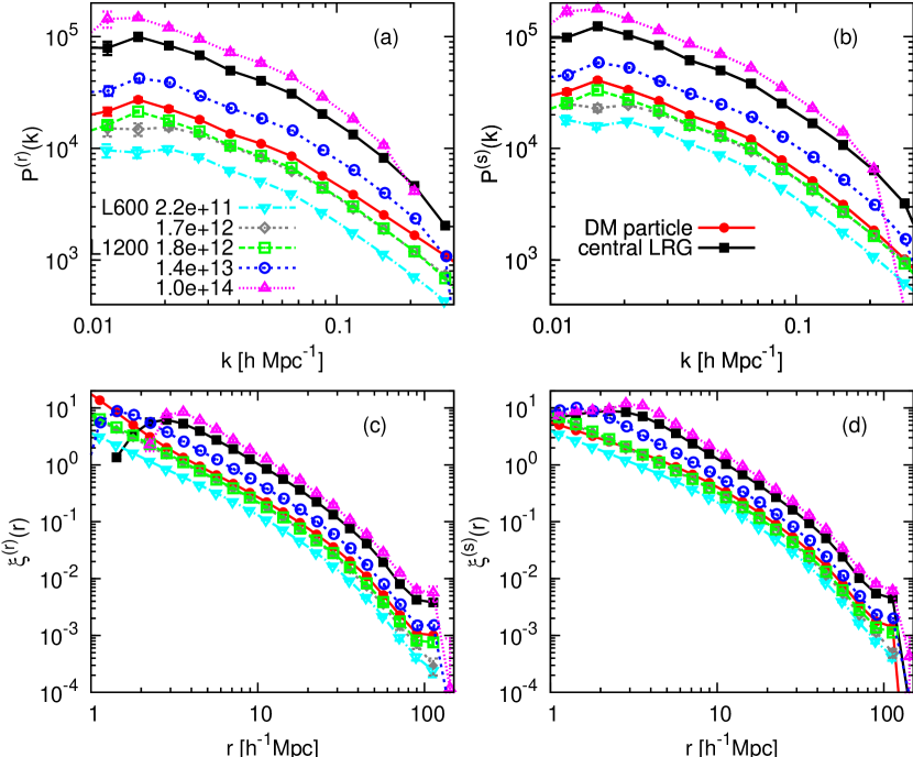
We plot the two-point statistics for dark matter halos, central LRGs, and dark matter particles measured from our simulation catalogs in Figure 1. When dark matter halos are analyzed, they are divided into narrow mass bins as $M_{i}-\Delta M_{i}<M_{i}<M_{i}+\Delta M_{i}$ for $i$th bin where $\Delta M_{i}=0.2M_{i}$. Corresponding ranges of the number of particles for each halo catalog are listed in Table 2. Results of LRGs and dark matter are shown only for the L1200 samples while those of high and low mass halos are shown for the L1200 and L600 samples, respectively. Results are averaged over all the realizations. In redshift space, positions of objects are displaced as a result of the peculiar velocity along the line of sight. We regard each direction along the three axes of simulation box as the line of sight and the statistics are averaged over three projections of all realizations for a total of 45 samples for the L600 simulation and 12 for the L1200 simulation. The error bars shown in Figure 1 are the standard error of the mean.

Figures 1 (a) and (b) show the power spectra in real space, $P^{(r)}(k)$, and in redshift space, $P^{(s)}(k)$, respectively. In both figures clear halo-mass dependence of the clustering amplitude can be found. The gray and green lines show the halo power spectra with the same halo mass in the L600 and L1200 samples, respectively. It can be easily seen that the agreement of the power spectra between the two boxes is very good for $k>0.03{\hbox{$~{}h{\rm~{}Mpc}^{-1}$}}$, indicating that resolution of a halo with $\geq 12$ particles is enough for the clustering analysis here. The discrepancy between the two lines at the smaller $k<0.03{\hbox{$~{}h{\rm~{}Mpc}^{-1}$}}$ is owing to the large cosmic variance effect in the L600 sample. Figures 1 (c) and (d) show the correlation functions in real space, $\xi^{(r)}(r)$, and in redshift space, $\xi^{(s)}(r)$, respectively. The suppression of the correlation functions for halos and central LRGs is caused by the finite size of the halos and it is alleviated to some extent in redshift space due to their random velocities (Jackson, 1972). The baryonic acoustic features, which were clearly detected in our simulation samples as a single peak at $\sim 100{\hbox{$~{}h^{-1}$}{\rm~{}Mpc}}$, appear as slight bumps in Figures 1 (c) and (d) because we use the binning much broader than the width of the peak.

The bias parameter can be computed both in Fourier space, $b(k)$, and in configuration space, $b(r)$, through

$$b(k)=\left(\frac{P^{(r)}(k)}{P^{(r)}_{m}(k)}\right)^{1/2},\ \ \ b(r)=\left(\frac{\xi^{(r)}(r)}{\xi^{(r)}_{m}(r)}\right)^{1/2}.$$ (2)

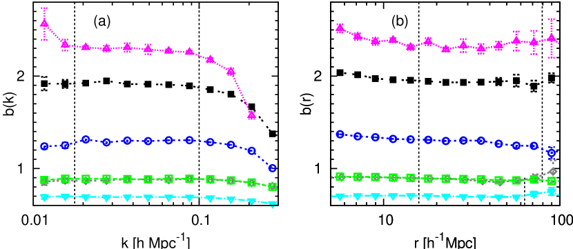
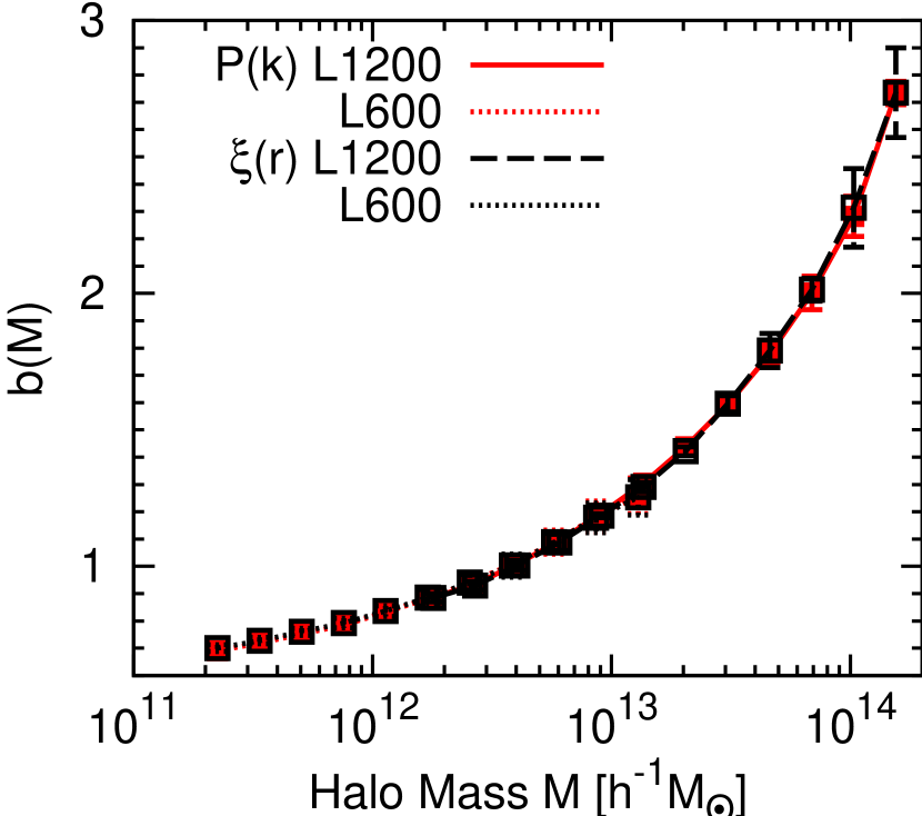
Figure 2 shows the $b(k)$ and $b(r)$ for dark matter halos and LRGs. The results are averaged over realizations and the error bars are the error of the mean. In both configuration and Fourier space, the bias parameters for halos and LRGs are found to be almost constant on sufficiently large scales. We assume the bias to be constant and search for the best fit value for each sample by computing the $\chi^{2}$ statistics. We compute $\chi^{2}$ for $16<r<79{\hbox{$~{}h^{-1}$}{\rm~{}Mpc}}$ in configuration space and for $0.018<k<0.10{\hbox{$~{}h{\rm~{}Mpc}^{-1}$}}$ in Fourier space for results from the L1200 simulations. On the other hand we compute it for $16<r<63{\hbox{$~{}h^{-1}$}{\rm~{}Mpc}}$ in configuration space for the L600 samples because the large-scale data is not very reliable owing to the cosmic variance while we still use the same range in Fourier space. Figure 3 shows the halo biasing as a function of the halo mass, $b(M)$. The error bars show the 95% confidence interval. The results between L600 and L1200 are largely overlapped with each other and we confirm that the systematic error caused by the different box sizes is negligibly small. In addition, the bias parameters obtained in Fourier and configuration space are consistent. The best fit values obtained here are used for the theoretical prediction of $\beta$ through Kaiser’s formula in Section 4.

3. Linear Theory of Redshift-space Distortions

There are at least two ways to determine the redshift distortion parameter $\beta$. They have been well developed both in Fourier space (Kaiser, 1987; Cole et al., 1994) and in configuration space (Hamilton, 1992) under the plane-parallel approximation and summarized in a review by Hamilton (1998), who also collected the observational constraints then available on $\beta$ in various surveys. We follow the similar notation with that adopted by Tinker et al. (2006).

3.1. Fourier Space

For plane-parallel redshift-space distortions, the redshift space power spectrum can be written as (Kaiser, 1987)

$$P^{(s)}(k,\mu_{\bf k})=P_{0}(k)L_{0}(\mu_{\bf k})+P_{2}(k)L_{2}(\mu_{\bf k})+P_{4}(k)L_{4}(\mu_{\bf k}),$$ (3)

where $L_{l}$ are Legendre Polynomials. The multipoles of the redshift-space power spectrum are expressed as

$$P_{l}(k)=\frac{2l+1}{2}\int^{+1}_{-1}P^{(s)}(k,\mu_{\bf k})L_{l}(\mu_{\bf k})d\mu_{\bf k}.$$ (4)

We can derive two useful combinations of them which are directly related to $\beta$, the ratio of the monopole to the real-space power spectrum $P^{(0/r)}$ and the quadrupole-to-monopole ratio $P^{(2/0)}$ (Cole et al., 1994);

$$P^{(0/r)}(k) \equiv \frac{P_{0}(k)}{P^{(r)}(k)}=1+\frac{2}{3}\beta+\frac{1}{5}\beta^{2},$$ (5)

$$P^{(2/0)}(k) \equiv \frac{P_{2}(k)}{P_{0}(k)}=\frac{\frac{4}{3}\beta+\frac{4}{7}\beta^{2}}{1+\frac{2}{3}\beta+\frac{1}{5}\beta^{2}}.$$ (6)

The last equality in the two equations holds only on large scales where linear theory can be applied.

Figure 2.— Halo bias (a) in Fourier space and (b) in configuration space. The color of each line corresponds to the one with the same color in Figure 1. The bias for the central LRGs is also plotted for comparison. Error bars are the standard error of the mean. The region enclosed by the two vertical lines shows the scales where we assume the scale-independent bias.

Figure 3.— Halo bias as a function of the halo mass. Shown is the best fit values for constant fits of $b$ between $15<r<80{\hbox{$~{}h^{-1}$}{\rm~{}Mpc}}$ (L1200) and $15<r<60{\hbox{$~{}h^{-1}$}{\rm~{}Mpc}}$ (L600) for $\xi(r)$ and $0.02<k<0.1{\hbox{$~{}h{\rm~{}Mpc}^{-1}$}}$ for $P(k)$. Results from the L1200 samples are shown for $1.4\times 10^{12}\leq M\leq 1.9\times 10^{14}M_{\odot}$ and those from the L600 samples for $1.8\times 10^{11}M\leq 1.6\times 10^{13}M_{\odot}.$ The error bars show the 95% confidence levels.

3.2. Configuration Space

The redshift-space correlation functions can be expressed similarly to the power spectra under the plane-parallel approximation as

$$\xi^{(s)}(r_{p},r_{\pi})=\xi_{0}(r)L_{0}(\mu)+\xi_{2}(r)L_{2}(\mu)+\xi_{4}(r)L_{4}(\mu),$$ (7)

where $r_{p}$ and $r_{\pi}$ are the separations perpendicular and parallel to the line of sight and $\mu$ is the cosine of the angle between the separation vector and the line of sight $\mu=\cos{\theta}=r_{\pi}/r$. The multipoles of the redshift-space correlation function are expressed as

$$\xi_{l}(r)=\frac{2l+1}{2}\int^{+1}_{-1}\xi^{(s)}(r_{p},r_{\pi})L_{l}(\mu)d\mu.$$ (8)

In linear theory, the ratio of the monopole to the real-space correlation function and the quadrupole-to-monopole ratio are related to the redshift distortion parameter $\beta$ on large scales (Hamilton, 1992);

$$\xi^{(0/r)}(r) \equiv \frac{\xi_{0}(r)}{\xi^{(r)}(r)}=1+\frac{2}{3}\beta+\frac{1}{5}\beta^{2},$$ (9)

$$\xi^{(2/0)}(r) \equiv \frac{\xi_{2}(r)}{\xi_{0}(r)-\bar{\xi_{0}}(r)}=\frac{\frac{4}{3}\beta+\frac{4}{7}\beta^{2}}{1+\frac{2}{3}\beta+\frac{1}{5}\beta^{2}},$$ (10)

where $\bar{\xi_{0}}(r)=(3/r^{3})\int^{r}_{0}\xi_{0}(r^{\prime})r^{\prime 2}dr^{\prime}$. When one wants to constrain the pairwise velocity dispersion of galaxies which becomes dominant on small scales, the real space correlation function is convolved with the distribution function of pairwise velocities to give the redshift space correlation function (Peebles, 1980), which is not the purpose of this paper (see, e.g., Peacock et al., 2001; Zehavi et al., 2002; Hawkins et al., 2003; Jing & Börner, 2004; Guzzo et al., 2008; Cabré & Gaztañaga, 2009). We will briefly discuss the effect of the pairwise velocities on $\beta$ reconstruction at Section 4.2.

4. Results and Discussion

4.1. $\beta$ Reconstruction

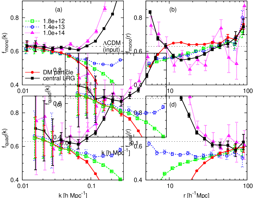
In Figure 4 we show the resulting $\beta$ values of dark matter halos, LRGs, and dark matter reconstructed by the methods described in Section 3. In each panel the horizontal lines show the large-scale values predicted by general relativity, $\beta=\Omega_{m}^{0.55}(z)/b$ (Linder, 2005). For the bias parameters in Fourier and configuration space we use the best fit values obtained in Figure 3. The $\beta$ value of dark matter is simply equal to the growth rate $f$ because $b=1$. We can see the agreement of the $\beta$ values obtained from the L600 and L1200 samples with the same halo mass, thus the different number of particles, indicating that resolution of a halo with 12 particles is accurate enough for $\beta$ reconstruction. The discrepancy between the two on large scales is again owing to the cosmic variance in the L600 sample.

Figure 4.— Redshift distortion parameter $\beta$ reconstructed from; (a) the monopole-to-real-space ratio of the power spectra; (b) the monopole-to-real-space ratio of the correlation functions; (c) the quadrupole-to-monopole ratio of the power spectrum; (d) the quadrupole-to-monopole ratio of the correlation functions. The horizontal lines represent the prediction from linear theory for each measurement with the same color and line type, where the best fit parameter for the biasing is used for the prediction. Error bars are the standard error of the mean. The diamonds and the open circles have been offset in the horizontally positive direction for clarity while the open squares and the triangles in the horizontally negative direction.

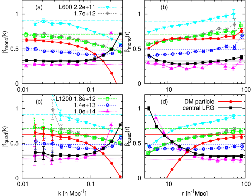
Figure 4 (a) shows $\beta$ as a function of $k$ measured from the ratio of the monopole to the real-space power spectrum $P^{(0/r)}=P_{0}/P^{(r)}$. Small-scale values obtained from the dark matter particles and small-mass halos are suppressed by the random peculiar velocities, while those from the LRGs and massive halos go up on such scales as a result of the finite size of halos, as described in Section 2.2. One can see that, for the most massive halos ($M\sim 10^{14}h^{-1}M_{\odot}$) and LRGs, the ratio $P^{(0/r)}$ reconstructs the $\beta$ values predicted by linear theory at $k<0.08{\hbox{$~{}h{\rm~{}Mpc}^{-1}$}}$. This means that linear theory is accurate enough to predict and constrain $\beta$ using such massive halos. On the other hand, the smaller halos we focus on, the more prominent scale dependence of $\beta$ we find even on large scales. This behavior of $\beta$ from the smaller mass halos is consistent with that obtained by Tinker et al. (2006). They used mock galaxies assigned to the halos by the HOD parameters applied to the SDSS MAIN galaxies (Zehavi et al., 2005) which preferentially reside in halos with small mass. Thus the behavior seen by Tinker et al. (2006) is found to be caused by the contribution from smaller halos. Note that here we used the real-space power spectrum measured from the simulations. It is not a direct observable and translation of the power spectrum from redshift space to real space usually draws the additional error.

Figure 4 (b) is the same as Figure 4 (a), but the $\beta$ values are measured as a function of separation $r$ computed from the ratio of the redshift-space and real-space correlation functions $\xi^{(0/r)}=\xi_{0}/\xi^{(r)}$. The slight difference of the linear theory prediction between Fourier and configuration space is due to the difference of the best fit parameters for the biasing seen in Figure 3. The scale dependence of the reconstructed $\beta$ found by using $\xi^{(0/r)}$ is more prominent than that by using $P^{(0/r)}$. Even the result obtained from the LRGs is monotonically increasing, intersects with the prediction from linear theory, and does not draw closer to a constant on all scales probed. A similar behavior has also been found for dark matter by Cabré & Gaztañaga (2009) up to $40{\hbox{$~{}h^{-1}$}{\rm~{}Mpc}}$ (see also the red line in Figure 4b), but the tendency is much more significant for dark matter halos, even for those with $b\sim 1$. Constraints on $\beta$ are usually given under the assumption of one constant parameter over a scale range for which the $\chi^{2}$ statistics is computed. However, according to Figure 4 (b), it could be a coincidence that one gets the true value of $\beta$ as a best fit parameter. Thus one should be cautious when the deviation from general relativity is investigated through the measurement of $\beta$ from the ratio $\xi_{0}/\xi^{(r)}$.

In measuring $\beta$ from the quadrupole-to-monopole ratio in Fourier space $P^{(2/0)}=P_{2}/P_{0}$, one needs to measure $P^{(s)}(k,\mu)$ in finite bins, usually constant separations in $\mu$, and numerically integrate it along $\mu$ direction. Hence the finite bin size may cause a systematic error in measurement of $\beta$. Using linear theory, we test the accuracy of the integration between constant $\mu$ and constant $\theta=\cos^{-1}{\mu}$ binnings. We found constant $\mu$ binning underestimates $\beta$ by 2.5% while constant $\theta$ binning overestimates by 1.3% for 10 bins. We thus adopt the constant $\theta$ binning and take the number of bin to be 10 between $0\leq\theta\leq 90^{\circ}$. Figure 4 (c) shows $\beta$ measured from the quadrupole-to-monopole moments $P^{(2/0)}$. This quantity can be directly measured in observation. We put artificial large-scale cuts in $\beta$ values measured from the L600 samples because they have limited number of modes and thus are strongly affected by the cosmic variance. We can see this by the difference between the green and gray lines because they have similar halo mass. On the other hand, we did not use such strong scale cuts in Figure 4 (a) because the effect of the cosmic variance can be eliminated to some extent by taking the ratio of two power spectra (McDonald & Seljak, 2009). In Fourier space, the behavior of $\beta$ measured from $P^{(2/0)}$ is almost the same as that from $P^{(0/r)}$ except for the magnitude of the error bars owing to the cosmic variance.

Finally, we show $\beta$ values measured from the quadrupole-to-monopole ratio in configuration space $\xi^{(2/0)}=\xi_{2}/\xi_{0}$ in Figure 4 (d). In measuring the quadrupole moment by equation (8) we adopt the binning on a polar grid of logarithmic spacing in $r$ and linear spacing in angle, then numerically integrate the correlation function at each $r$, as was done by Tinker et al. (2006). On small scales, the behavior of $\beta$ thus determined is complicated. For small halos, the results give lower $\beta$ values than those from linear theory prediction, which may be caused by the random peculiar velocities and thus might be correctable to some extent (see Hawkins et al., 2003; Tinker et al., 2006). However, note that peculiar velocities predicted from a simple halo model (Yang et al., 2003) have very different luminosity dependence with those from observations (Jing & Börner, 2004; Li et al., 2006, see also Slosar et al. 2006). For the massive halos, the $\beta$ values on small scales are larger than the linear theory prediction, which might indicate that these halos are approaching with each other. Interestingly, for the most massive halos ($1.0\times 10^{14}h^{-1}M_{\odot}$) and the LRG sample, we can simply use linear theory and use the data points on scales larger than $\sim 25{\hbox{$~{}h^{-1}$}{\rm~{}Mpc}}$ in order to constrain the growth rate. For galaxies within the halos with the mass $\sim 1.4\times 10^{13}h^{-1}M_{\odot}$, the $\beta$ value is coincidently a constant, but it is lower than the linear theory prediction. If we use a population of such galaxies, we would underestimate the growth factor. Lastly for galaxies within less massive halos, the reconstructed $\beta$ becomes a scale-dependent function, and one has to be extremely careful in extracting the linear growth factor from a measurement of redshift-space distortions of such galaxies.

Figure 5.— Quadrupole-to-monopole ratio in Fourier space for dark matter particles (red) and for massive (magenta) and small (light blue) halos. The horizontal lines are the linear theory prediction. The upper and lower dashed curves in red are the non-linear prediction with the pairwise velocity dispersion $\sigma_{v}=500$ and $600{\rm km/s}$, respectively, while those for halos are with $\sigma_{v}=400$ and $500{\rm km/s}$.

4.2. Pairwise Velocity Dispersion

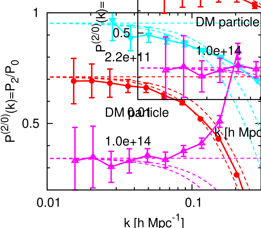
In order to see if random peculiar velocities can cause the deviation from the linear theory prediction, we consider a simple Exponential model for the pairwise velocity dispersion (PVD) in configuration space which results in a Lorentz damping factor in Fourier space,

$$G(k,\mu_{\bf k},\sigma_{v})=(1+k^{2}\mu^{2}_{\bf k}\sigma^{2}_{v}/2)^{-1}.$$ (11)

The power spectrum of this dispersion model is expressed as Equation (1) multiplied by $G(k,\mu_{\bf k},\sigma_{v})$. Although more accurate models have been developed by many authors, this simple model is useful enough for our purpose. In Figure 5, we show the predictions for the quadrupole-to-monopole ratio in Fourier space $P^{(2/0)}$ from the dispersion model. In order to avoid making the figure unclear, we show the results for only dark matter particles, the most massive halos and the smallest halos. The overall shape of $P^{(2/0)}$ for dark matter is well explained by the dispersion model with $\sigma_{v}\sim 600$ km/s, which has already been found using more accurate models (e.g., Taruya et al., 2010). However, the results for dark matter halos are much more complicated. Here we adopt $\sigma_{v}\sim 450$ km/s for the halos according to (Hamana et al., 2003). For small halos, not only the deviation of the measurement from the linear theory prediction but also its scale dependence cannot be corrected by the model. On the other hand, the behavior of $\beta$ reconstructed for massive halos is opposite to the dispersion model. These complex results are somewhat expected because the halo peculiar velocities change very mildly with their mass (Hamana et al., 2003). Thus the difference of the scale dependences of $\beta$ among small and large halos cannot be simultaneously explained with such analytical models for the PVD. We note that the model of PVD was adopted by Guzzo et al. (2008) to correct for the nonlinear effect when they measure the $\beta$ at redshift 0.8.

Figure 6.— Joint probability distributions of overdensity fields for dark halos with dark matter overdensity in real space (left panels) and in redshift space (right panels) smoothed over $R_{s}=20{\hbox{$~{}h^{-1}$}{\rm~{}Mpc}}$ and $R_{s}=30{\hbox{$~{}h^{-1}$}{\rm~{}Mpc}}$. Upper, middle, and lower panels in each set show the results for halos with $M=1.9\times 10^{11}$, $M=1.4\times 10^{12}$, and $M>1.9\times 10^{13}$, respectively. The values in the color bars show the logarithm of the probability to base 10. The solid lines are the conditional mean $\bar{\delta}(\delta_{m})$. The dashed lines show the linear bias relation $\delta(\delta_{m})=b_{{\rm var}}\delta_{m}$.

Figure 7.— Dependence of $r_{{\rm corr}}$, $\epsilon_{{\rm nl}}$, and $\epsilon_{{\rm scatt}}$ in real space (left panels) and in redshift space (right panels) smoothed over $R_{s}=20{\hbox{$~{}h^{-1}$}{\rm~{}Mpc}}$ and $R_{s}=30{\hbox{$~{}h^{-1}$}{\rm~{}Mpc}}$. The red points show the results obtained from the L600 samples while the black points the L1200 samples. Error bars are the standard error of the mean.

4.3. Nonlinear Stochastic Biasing

In the derivation of Kaiser’s effect, the linear bias relation between objects considered (galaxies or halos) and dark matter was assumed. However, there could be considerable stochasticity and nonlinearity in the bias relation between dark halos (or galaxies) and dark matter (Dekel & Lahav, 1999). We follow the formalism proposed by Taruya & Suto (2000) and applied to simulation data by Yoshikawa et al. (2001). We briefly summarize some parameters defined by Taruya & Suto (2000) to quantify the nonlinearity and stochasticity of the halo bias. First, the density fields of dark matter and dark halos are evaluated as $\delta_{m}({\bf x},R_{S})$ and $\delta({\bf x},R_{S})$, respectively, smoothed over the top-hat window radius $R_{s}$. The bias parameter and the correlation coefficient are respectively defined by

$$b_{{\rm var}}\equiv\sqrt{\frac{\left\langle\delta^{2}\right\rangle}{\left\langle\delta_{m}^{2}\right\rangle}},\ \ \ r_{{\rm corr}}\equiv\frac{\left\langle\delta\delta_{m}\right\rangle}{\sqrt{\left\langle\delta^{2}\right\rangle\left\langle\delta_{m}^{2}\right\rangle}}.$$ (12)

Note that the bias parameters defined in Section 2.2 are from the two-point statics, while the bias $b_{{\rm var}}$ defined here is from one-point statistics. In order to quantify the nonlinear and stochastic nature of the biasing separately, two more useful parameters are introduced. For this purpose, let us define the conditional mean of $\delta$ for a given $\delta_{m}$,

$$\bar{\delta}(\delta_{m})=\int\delta\ P(\delta|\delta_{m})d\delta,$$ (13)

where $P(\delta|\delta_{m})$ is the conditional probability distribution function. Then the nonlinearity of the biasing is quantified by

$$\epsilon_{{\rm nl}}\equiv\frac{\left\langle\delta^{2}_{m}\right\rangle\left\langle\bar{\delta}^{2}\right\rangle}{\left\langle\bar{\delta}\delta_{m}\right\rangle^{2}}-1,$$ (14)

which vanished only when the biasing is linear. Similarly, the stochasticity of the biasing is characterized by

$$\epsilon_{{\rm scatt}}\equiv\frac{\left\langle\delta^{2}_{m}\right\rangle\left\langle(\delta-\bar{\delta})^{2}\right\rangle}{\left\langle\bar{\delta}\delta_{m}\right\rangle^{2}},$$ (15)

which vanishes for the deterministic bias where $\delta=\bar{\delta}(\delta_{m})$.

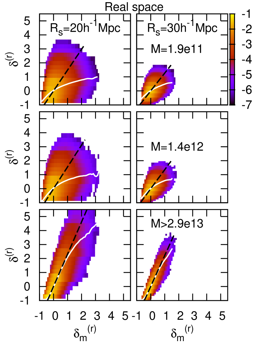
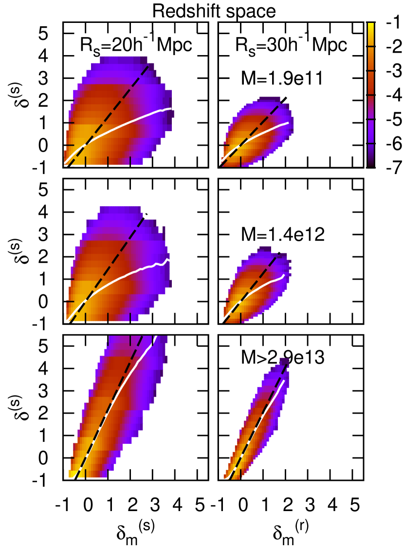
Following the same procedure of Yoshikawa et al. (2001), we compute the parameters defined above for our halo catalogs in real and redshift space. In order to minimize the Poisson noise effect and fairly compare the results of different mass, only in this subsection we keep each subsample of a given halo mass to have the same number density, $1.16\times 10^{-4}(h^{-1}{\rm Mpc})^{-3}$. This density corresponds to $N_{{\rm halo}}\approx 2.5\times 10^{4}$ for L600 samples and $N_{{\rm halo}}\approx 2.0\times 10^{5}$ for L1200 samples. We adopt the smoothing scales $R_{s}=20$ and 30$~{}h^{-1}$ Mpc. Many pairs of the values $[\delta({\bf x}),\delta_{m}({\bf x})]$ are obtained for randomly selected points ${\bf x}$ in the simulation box.

In Figure 6, we show the joint distribution of $\delta$ with $\delta_{m}$ in real space (left) and in redshift space (right). From the top to bottom, the results obtained from the smallest mass bin of the L600 samples ($M=1.9\times 10^{11}h^{-1}M_{\odot}$), the smallest mass bin of the L1200 samples ($M=1.4\times 10^{12}h^{-1}M_{\odot}$), and the largest mass bin of the L1200 samples ($M>2.9\times 10^{13}h^{-1}M_{\odot}$) are plotted. In each panel we also plot the conditional mean relation $\bar{\delta}(\delta_{m})$ as the solid line and the linear bias relation $\delta=b_{{\rm var}}\delta_{m}$ as the dashed line, both of which are obtained from our simulations. Here we focus on halo mass dependence of the nonlinear stochastic biasing. The deviation of $\bar{\delta}$ from the linear bias is caused by the nonlinear stochastic bias as well as the halo exclusion effect (Yoshikawa et al., 2001, see also Smith et al. 2007). The halo exclusion effect is alleviated in redshift space due to the random velocities of halos, as we have seen in Section 2.2. Despite the fact that this exclusion effect is more significant for larger thus more massive halos, the deviation from the linear relation for such halos is much smaller. This indicates that more massive halos have the smaller nonlinearity and stochasticity, and the latter was also found by Hamaus et al. (2010) using a complementary statistics in real space.

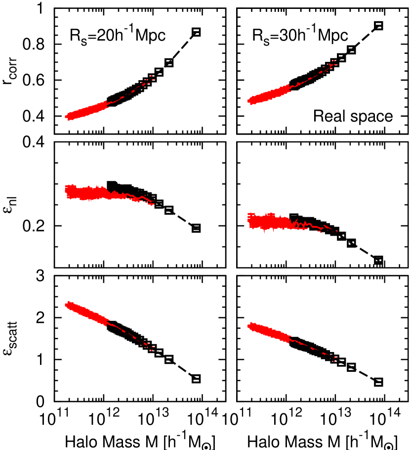
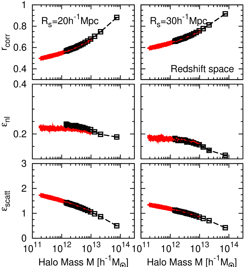
In order to see these effects more quantitatively, we show $r_{{\rm corr}}$, $\epsilon_{{\rm nl}}$, and $\epsilon_{{\rm scatt}}$ as functions of halo mass in Figure 7 from the top to bottom. The results for the parameter $\epsilon_{{\rm nl}}$ show that the nonlinearity of the halo biasing is smallest for the most massive halos. It increases for smaller halos and gets close to a constant. Similarly, the stochasticity parameter $\epsilon_{{\rm scatt}}$ has the minimum value for the most massive halos. At a whole mass range probed, however, the stochastic bias monotonically increases toward the lowest mass. Finally the stochasticity of the smallest halos becomes five times larger than that of the most massive halos. Thus both the nonlinearity and stochasticity of the halo biasing, particularly the latter, is likely one of the cause for the systematic deviation of $\beta$ values from the theoretical prediction.

4.4. Halo Mass Dependence of Growth Rate Constraints

Because we also calculated the power spectra and correlation functions for dark matter particles in the same samples as those for dark matter halos and LRGs, we can directly reconstruct the growth rate through

$$f(r)=b(r)\beta(r) = \left[\frac{\xi^{(r)}(r)}{\xi^{(r)}_{m}(r)}\right]^{1/2}\beta(r),$$ (16)

$$f(k)=b(k)\beta(k) = \left[\frac{P^{(r)}(k)}{P^{(r)}_{m}(k)}\right]^{1/2}\beta(k).$$ (17)

The difference between the use of $\beta$ and $f$ is just whether the bias $b$ is used as prediction or measurement. When $f$ is used, however, we can take into account the slight scale dependence of the bias seen in Figure 2. Figures 8 show the growth rate measured from the four methods described above. The horizontal line shows the input $\Lambda$CDM model predicted from general relativity $f=\Omega_{m}^{0.55}(z)$ (Linder, 2005). We can also see that the linear redshift distortions for the LRGs reconstruct the true value of $f$ well, except for that from $\xi^{(0/r)}$.

Figure 8.— Same as Figure 4 but for growth rate $f$, reconstructed from; (a) the monopole-to-real-space ratio of the power spectra; (b) the monopole-to-real-space ratio of the correlation functions; (c) the quadrupole-to-monopole ratio of the power spectrum; (d) the quadrupole-to-monopole ratio of the correlation functions. The horizontal line shows the linear theory prediction, $\Omega_{m}^{0.55}(z)$. Error bars are the standard error of the mean. The open squares and the open circles have been offset in the horizontally negative direction for clarity while the triangles in the horizontally positive direction.

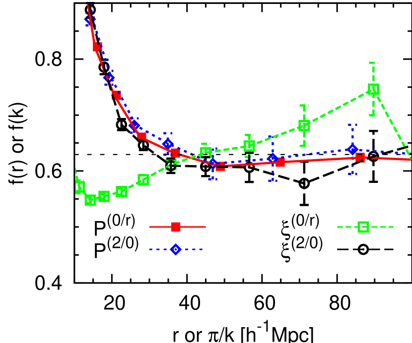
Here let us discuss which method can be used to obtain the growth factor $f$ better. Figure 9 shows the comparison among the 4 methods for the measurement of $f$ from the LRG clustering. As we have seen above, we find strong scale dependence of the growth factor obtained from $\xi^{(0/r)}$. On the other hand, both of the methods in Fourier space, $P^{(0/r)}$ and $P^{(2/0)}$, and the estimator $\xi^{(2/0)}$ in configuration space, can give good estimation of $\beta$ in linear theory on scales $\lambda\equiv\pi/k>30{\hbox{$~{}h^{-1}$}{\rm~{}Mpc}}$ or $r>30{\hbox{$~{}h^{-1}$}{\rm~{}Mpc}}$.

Figure 9.— Comparison of the growth rate measurement from LRGs among the different methods. The horizontal axis shows separation $r$ for configuration space measurement while $\pi/k$ for Fourier space measurement. The diamonds/filled squares have been offset in the horizontally negative/positive direction for clarity.

5. Conclusion

We have investigated how accurately the redshift-space distortions can be used to measure the linear growth factor $f$. The growth factor is a powerful observable targeted by future large redshift surveys to probe dark energy and to distinguish among different gravity theories. For this purpose, we constructed a large set of $N$-body simulations, dividing each dark matter halo catalog into the subsamples with narrow mass ranges. As an example of a galaxy sample, mock SDSS LRG catalogs were constructed by applying the HOD modeling to the simulated halos. Then we have measured the two-point statistics, power spectra and correlation functions, for dark matter halos and LRGs. The dark matter halos were analyzed as a function of halo mass in order to see dependence of the $\beta$ measurement on the halo mass.

We have determined the $\beta$ values as a function of halo mass and scale using four methods. First, we found that $\beta$ reconstructed from the ratio of the monopole to the real-space power spectra $P^{(0/r)}=P^{(s)}/P^{(r)}$ (equation (5)) asymptotically approaches the true value. In particular for the massive halos and LRGs, the prediction from linear theory known as Kaiser’s formula is applicable to give a correct constraint on the growth rate. However, for less massive halos, the ratio approaches the true value only at a very large scale $k<0.02{\hbox{$~{}h{\rm~{}Mpc}^{-1}$}}$. Second, $\beta$ reconstructed from the ratio of the monopole to the real-space correlation function $\xi^{(0/r)}=\xi^{(s)}/\xi^{(r)}$ (equation (9)) approaches neither the true value nor a constant even on large scales. This statement is valid especially for small halos with the bias parameter $b\leq 1$. Because the growth rate is assumed to be a constant when modified gravity theories are tested, the ratio $\xi^{(s)}/\xi^{(r)}$ cannot be used in a simple way for this purpose. Third, the quadrupole-to-monopole ratio in Fourier space $P^{(2/0)}=P_{2}/P_{0}$ (equation (6)) gives almost the same value of $\beta$ as $P^{(0/r)}$ but with larger error bars as expected. Finally, we found that when the quadrupole-to-monopole ratio in configuration space $\xi^{(2/0)}=\xi_{2}/\xi_{0}$ (equation (10)) is used, a similar conclusion is reached to that of $P^{(2/0)}$ when $r=\lambda=\pi/k$ is adopted.

For small halos with $b\leq 1.3$, the reconstructed $\beta$ values do not approach a constant in most of measurable regions, particularly those from $\xi^{(0/r)}$ in the configuration space. No method can provide a reliable estimator for the determination of the growth factor from the clustering of such small halos on the large range of scales probed. Using the halo catalogs with different box sizes, we confirmed that such a behavior is not caused by the resolution effect of small dark matter halos. While the scale dependence changes with the halo mass, the peculiar velocity of halos does not change much with the mass (Hamana et al., 2003). Using the simple dispersion model, we demonstrated that the different scale dependence of $\beta$ among small and large halos cannot be simultaneously explained. Also there are two types of velocity biases which affect the redshift distortion; the dynamical bias caused by dynamical friction and the spatial bias caused by the difference between the distribution of halos and that of dark matter. There is no dynamical velocity bias because the halo velocities are determined from the mean velocities of dark matter within the halos in our analysis. The spatial velocity bias should exist, which is coupled with the nonlinear stochastic bias discussed in the text.

On the other hand, it is known that the clustering of small dark matter halos depends not only on their mass but also on their assembly history, so called the assembly bias (e.g., Gao et al., 2005). Wang et al. (2007) showed that old and low-mass halos that are preferentially associated with a high density field are more strongly clustered than young halos with the same mass, and consequently have higher velocities. Besides, the stochasticity between halos and dark matter is (Dekel & Lahav, 1999) can be a source of the systematic errors in the $\beta$ reconstruction. Using a method introduced by Taruya & Suto (2000) and applied to simulation data by Yoshikawa et al. (2001), we have found that both the nonlinearity and the stochasticity of small halos become larger than massive halos. Particularly the stochastic bias monotonically increases as the mass of halos decreases, as was found in real space by Hamaus et al. (2010) using the two-point statistics. Thus the strong scale dependence of $\beta$ for low mass halos could be caused by the assembly and/or nonlinear stochastic bias. However fortunately, the scale dependence of the measured $\beta$ weakens with the increase of halo mass. For massive halos with $b>1.5$, the measured $\beta$ approaches the constant predicted by Kaiser’s formula on scales $k<0.08{\hbox{$~{}h{\rm~{}Mpc}^{-1}$}}$ or $r>30{\hbox{$~{}h^{-1}$}{\rm~{}Mpc}}$.

Because the analysis of redshift-space distortions is powerful to investigate not only properties of dark energy but also modified gravity theories, it will keep on playing a key role in ongoing and upcoming large redshift surveys, such as BOSS, FMOS, HETDEX, WiggleZ, and BigBOSS. Galaxies targeted by the BOSS survey are luminous red galaxies, which reside in massive halos. In this work we demonstrate the $\beta$ value can be well reconstructed with a redshift distortion analysis of LRGs. On the other hand, one of the samples targeted by the BigBOSS, for example, is that of emission-line galaxies, which reside in halos with a broad range of halo mass. One needs to be careful in using such a sample to constrain the growth rate from the redshift distortion, because it can be a scale-dependent function. While one might be able to obtain a result consistent (or inconsistent) with the prediction from general relativity, it could be just a coincidence after the scale-dependent growth rate is averaged over some separation or wavenumber ranges. We will use semi-analytical modeling or a halo occupation model to investigate this issue in future work.

Recently, an interesting method was proposed by Seljak et al. (2009) to suppress the shot noise in power spectrum measurement. They considered an optimal weighting function $f(M)$ in measuring the galaxy overdensity, where they give higher weights on higher mass halos. Compared with our results presented here, such a mass weighting scheme is useful not only for suppressing the shot noise but also obtaining the true value of the growth rate. This scheme can be naturally incorporated into our method and such a study will be presented in our future paper. Another theoretical improvement to be applied for observation is evading the cosmic variance limit, which is one of the most important tasks for precise measurement of the redshift-space distortions, as we have already seen above. McDonald & Seljak (2009) showed using multiple tracers of density with different biases suppresses the noise for measurement of $\beta$ on large scales dramatically compared to the traditional single tracer method (see also White et al., 2009; Gil-Marín et al., 2010). But the different scale-dependent properties of $\beta$ for different halo masses found in Figure 4 imply that the real situation might be more complex, and realistic models of galaxies must be adopted to investigate if the method of multiple tracers works.

References

- Amendola et al. (2005) Amendola, L., Quercellini, C., & Giallongo, E. 2005, MNRAS, 357, 429
- Berlind & Weinberg (2002) Berlind, A. A., & Weinberg, D. H. 2002, ApJ, 575, 587
- Berlind et al. (2001) Berlind, A. A., Narayanan, V. K. & Weinberg, D. H. 2001, MNRAS, 549, 688
- Cabré & Gaztañaga (2009) Cabré, A., & Gaztañaga, E. 2009, MNRAS, 393, 1183
- Carroll et al. (2004) Carroll, S. M., Duvvuri, V., Trodden, M., & Turner, M. S. 2004 Phys. Rev. D, 70, 043528
- Cole et al. (1994) Cole, S., Fisher, K. B., & Weinberg, D. H., 1994, MNRAS, 267, 785
- da Angela et al. (2008) da Angela, J., et al. 2008, MNRAS, 383, 565
- Daniel et al. (2010) Daniel, S. F., Linder, E. V., Smith, T. L., Caldwell, R. R., Cooray, A., Leauthaud, A., & Lombriser, L. 2010, Phys. Rev. D, 81, 123508
- Dekel & Lahav (1999) Dekel, A., & Lahav, O. 1999, ApJ, 520, 24
- Desjacques & Sheth (2010) Desjacques, V., & Sheth, R. K. 2010, Phys. Rev. D, 81, 023526
- Di Porto & Amendola (2008) Di Porto, C., & Amendola, L. 2008, Phys. Rev. D, 77, 083508
- Dvali et al. (2000) Dvali, G., Gabadadze, G., & Porrati, M. 2000, Phys. Lett. B, 485, 208
- Eisenstein et al. (2001) Eisenstein, D. J. et al. 2001, AJ, 122, 2267
- Gao et al. (2005) Gao, L., Springel, V., & White, S. D. M. 2005, MNRAS, 363, L66
- Gil-Marín et al. (2010) Gil-Marín, H., Wagner, C., Verde, L., Jimenez, R., & Heavens, A. F. 2010, MNRAS, 407. 772
- Glazebrook et al. (2007) Glazebrook, K., et al. 2007, arXiv:astro-ph/0701876
- Guzzo et al. (2008) Guzzo, L., et al. 2008, Nature, 451, 541
- Hamana et al. (2003) Hamana, T., Kayo, I., Yoshida, N., Suto, Y., & Jing, Y. P. 2003, MNRAS, 343, 1312
- Hamaus et al. (2010) Hamaus, N., Seljak, U., Desjacques, V., Smith, R. E., & Baldauf, T. 2010, Phys. Rev. D, 82, 043515
- Hamilton (1992) Hamilton, A. J. S. 1992, ApJ, 385, 5
- Hamilton (1998) Hamilton, A. J. S. 1998, in The Evolving Universe: Selected Topics on Large-scale Structure and on the Properties of Galaxies, ed. D. Hamilton (Dordrecht: Kluwer), 185
- Hatton & Cole (1998) Hatton, S., & Cole, S. 1998, MNRAS, 296, 10
- Hatton & Cole (1999) Hatton, S., & Cole, S. 1999, MNRAS, 310, 1137
- Hawkins et al. (2003) Hawkins, E., et al. 2003, MNRAS, 346, 78
- Hill et al. (2004) Hill, G. J., Gebhardt, T., Komatsu, E., & MacQueen, P. J. 2004, in AIP Conf. Proc., 743, The New Cosmology: Conference on String and Cosmology (New York: AIP), 224
- Hu & Haiman (2003) Hu, W., & Haiman, Z. 2003, Phys. Rev. D, 68, 063004
- Jackson (1972) Jackson, J. C. 1972, MNRAS, 156, 1
- Jennings et al. (2010) Jennings, E., Baugh, C. M., & Pascoli, S. 2010, arXiv:1003.4282 [astro-ph.CO]
- Jing & Börner (2004) Jing, Y. P., & Börner, G. 2004, ApJ, 617, 782
- Jing et al. (1998) Jing, Y. P., Mo, H. J., & Börner, G. 1998, ApJ, 494, 1
- Jing et al. (2007) Jing, Y. P., Suto, Y., & Mo, H. J. 2007, ApJ, 657, 664
- Kaiser (1984) Kaiser, N. 1984, ApJ, 284, L9
- Kaiser (1987) Kaiser, N. 1987, MNRAS, 227, 1
- Komatsu et al. (2010) Komatsu, E., et al. 2010, arXiv:1001.4538 [astro-ph.CO]
- Li et al. (2006) Li, C., Jing, Y. P., Kauffmann, G., Börner, G., White, S. D. M., & Cheng, F. Z. 2006, MNRAS, 368, 37
- Linder (2005) Linder, E. V. 2005, Phys. Rev. D, 72, 043529
- Matsubara (2004) Matsubara, T. 2004, ApJ, 615, 573
- McDonald & Seljak (2009) McDonald, P., & Seljak, U. 2009, J. Cosmology Astropart. Phys, 10, 007
- Nakamura et al. (2009) Nakamura, G., Hütsi, G., Sato, T., & Yamamoto, K. 2009, Phys. Rev. D, 80, 123524
- Nesseris & Perivolaropoulos (2008) Nesseris, S., & Perivolaropoulos, L. 2008, Phys. Rev. D, 77, 023504
- Okumura et al. (2009) Okumura, T., Jing, Y. P., & Li, C. 2009, ApJ, 694, 214
- Okumura et al. (2008) Okumura, T., Matsubara, T., Eisenstein, D., Kayo, I., Hikage, C., Szalay, A. S., & Schneider, D. P. 2008, ApJ, 676, 889
- Peacock & Dodds (1994) Peacock, J. A., & Dodds, S. 1994, MNRAS, 267, 1020
- Peacock et al. (2001) Peacock, J. A., et al. 2001, Nature, 410, 169
- Peebles (1980) Peebles, P. J. E. 1980, The Large-Scale Structure of the Universe (Princeton: Princeton Univ. Press)
- Percival & White (2009) Percival, W. J., & White, M. 2009, MNRAS, 393, 297
- Perlmutter et al. (1999) Perlmutter, S., et al. 1999, ApJ, 517, 565
- Reyes et al. (2010) Reyes, R., Mandelbaum, R., Seljak, U., Baldauf, T., Gunn, J. E., Lombriser, L., & Smith, R. E. 2010, Nature, 464, 256
- Riess (1998) Riess, A. G., et al. 1998, AJ, 116, 1009
- Ross et al. (2007) Ross, N. P., et al. 2007, MNRAS, 381, 573
- Schlegel et al. (2009a) Schlegel, D. J., White, M., & Eisenstein, D. J. 2009a, arXiv:0902.4680 [astro-ph.CO]
- Schlegel et al. (2009b) Schlegel, D. J., et al. 2009b, arXiv:0904.0468 [astro-ph.CO]
- Scoccimarro (2004) Scoccimarro, R., 2004, Phys. Rev. D, 70, 083007
- Scoccimarro et al. (2001) Scoccimarro, R., Sheth, R. K., Hui, L., & Jain, B. 2001, ApJ, 546, 20
- Seljak (2000) Seljak, U. 2000, MNRAS, 318, 203
- Seljak et al. (2009) Seljak, U., Hamaus, N., & Desjacques, V. 2009, Phys. Rev. Lett., 103, 091303
- Seljak & Zaldarriaga (1996) Seljak, U., & Zaldarriaga, M. 1996, ApJ, 469, 437
- Seo & Eisenstein (2003) Seo, H.-J., & Eisenstein, D. J. 2003, ApJ, 598, 720
- Seo et al. (2008) Seo, H.-J., Eisenstein, D. J., & Zehavi, I. 2008, ApJ, 681, 998
- Slosar et al. (2006) Slosar, A., Seljak, U., & Tasitsiomi, A. 2006, MNRAS, 366, 1455
- Smith et al. (2007) Smith, R. E., Scorrimarro, R., & Sheth, R. K. 2007, Phys. Rev. D, 75, 063512
- Song & Kayo (2010) Song, Y.-S., & Kayo, I. 2010, MNRAS, 407, 1123
- Spergel et al. (2003) Spergel, D. N., et al. 2003, ApJS, 517, 565
- Sumiyoshi et al. (2009) Sumiyoshi, M., et al. 2009, arXiv:0902.2064 [astro-ph.CO]
- Taruya & Suto (2000) Taruya, A., & Suto, Y. 2000, ApJ, 542, 559
- Taruya et al. (2010) Taruya, A., Nishimichi, T., & Saito, S. 2010, Phys. Rev. D, 82, 063522
- Taruya et al. (2009) Taruya, A., Nishimichi, T., Saito, S., & Hiramatsu, T. 2009, Phys. Rev. D, 80, 123503
- Tegmark et al. (2004) Tegmark, M., et al. 2004, ApJ, 606, 702
- Tegmark et al. (2006) Tegmark, M., et al. 2006, Phys. Rev. D, 74, 123507
- Tinker et al. (2006) Tinker, J. L., Weinberg, D. H., & Zheng, Z. 2006, MNRAS, 368, 85
- Wang et al. (2007) Wang, H. Y., Mo, H. J., & Jing, Y. P. 2007, MNRAS, 375, 633
- White et al. (2009) White, M., Song, Y.-S., & Percival, W. J. 2009, MNRAS, 397, 1348
- Yamamoto et al. (2008) Yamamoto, K., Sato, T., & Hütsi, G. 2008, Prog. Theor. Phys., 120, 609
- Yang et al. (2003) Yang, X. H., Mo, H. J., & van den Bosch, F. C. 2003, MNRAS, 339, 1057
- York et al. (2000) York, D. G. et al. 2000, AJ, 120, 1579
- Yoshikawa et al. (2001) Yoshikawa, K., Taruya, A., Jing, Y. P., & Suto, Y. 2001, ApJ, 558, 520
- Zehavi et al. (2002) Zehavi, I., et al. 2002, ApJ, 571, 172
- Zehavi et al. (2005) Zehavi, I., et al. 2005, ApJ, 630, 1
- Zhang et al. (2007) Zhang, P., Liguori, M., Bean, R., & Dodelson, S. 2007, Phys. Rev. Lett., 99, 141302
- Zheng et al. (2009) Zheng, Z., Zehavi, I., Eisenstein, D. J., Weinberg, D. H., & Jing, Y. P. 2009, ApJ, 707, 554
- Zheng et al. (2005) Zheng, Z., et al. 2005, ApJ, 633, 791