Products of random matrices and generalised quantum point scatterers

Abstract.

To every product of $2\times 2$ matrices, there corresponds a one-dimensional Schrödinger equation whose potential consists of generalised point scatterers. Products of random matrices are obtained by making these interactions and their positions random. We exhibit a simple one-dimensional quantum model corresponding to the most general product of matrices in $\text{SL}\left(2,{\mathbb{R}}\right)$. We use this correspondence to find new examples of products of random matrices for which the invariant measure can be expressed in simple analytical terms.

1. Introduction

Products of random $2\times 2$ matrices arise in many physical contexts: in the study of random spin chains, or when calculating the distribution of the natural frequencies of a classical random spring chain, or more generally when considering the propagation of a wave in a one-dimensional disordered medium [6, 31, 32]. It is often the case that, in the presence of disorder (i.e. randomness), the waves become sharply localised in space. This physical phenomenon is known as Anderson localisation; one of its mathematical manifestations is the exponential growth of the product of random matrices.

The rate of growth is called the Lyapunov exponent; it often has a physical interpretation in terms of the exponential decay of the transmission probability as the size of the disordered region grows. One method for calculating the Lyapunov exponent is based on a general theory developed by Furstenberg and others [6, 9, 20]. This method requires the explicit knowledge of a certain measure on the projective space, invariant under the action of the matrices in the product. Examples of products of random matrices for which this invariant measure can be obtained in analytical form are, however, very few; see for instance [6, 10, 27, 33] and the references therein.

The calculation of the Lyapunov exponent need not always make use of this invariant measure. There are alternative approaches; see for instance [32, 35, 36]. Nevertheless, the problem of determining the invariant measure is interesting in itself, and the present paper will focus on the presentation of new explicit examples from corresponding examples of exactly solvable models of one-dimensional disordered systems with point scatterers [2, 3, 38]. In our context, the phrase “exactly solvable” means that the calculation of the Lyapunov exponent associated with the disordered system is reduced to a problem of quadrature. Some of the models were solved by Nieuwenhuizen [35] (without the use of the invariant measure); some of them are, apparently, new. Although the work reported here is, for the most part, mathematically driven, these new models are of independent physical interest. To the best of our knowledge, all the explicit formulae for the invariant measures constitute new results. In the remainder of this introductory section, we review some relevant concepts and some known facts, summarise our main results, and give a sketch of our approach.

1.1. Products of random matrices

Let

$$A_{1},\,A_{2},\,A_{3},\,\cdots$$

denote independent, identically-distributed $2\times 2$ matrices with unit determinant, let $\mu$ be their common distribution, and consider the product

(1.1) $$\Pi_{n}:=A_{n}A_{n-1}\cdots A_{1}\,.$$

The number

(1.2) $$\gamma_{\mu}:=\lim_{n\rightarrow\infty}\frac{{\mathbb{E}}\left(\ln\left|\Pi_{n}\right|\right)}{n}$$

where $|\cdot|$ denotes the norm on matrices induced by the euclidean norm on vectors, also denoted $|\cdot|$, is called the Lyapunov exponent of the product.

The product grows if the angle between the columns decreases or, equivalently, if the columns tend to align along some common direction. In precise mathematical terms, a direction in ${\mathbb{R}}^{d}$ is a straight line through the origin, and the set of all directions is, by definition, the projective space $P\left({\mathbb{R}}^{d}\right)$. The case $d=2$ is particularly simple: any direction

$$\left\{\lambda\begin{pmatrix}x\\ y\end{pmatrix}\,:\;\lambda\in{\mathbb{R}}\right\}\,,$$

is characterised by the reciprocal, say

$$z=\frac{x}{y}\in\overline{\mathbb{R}}:={\mathbb{R}}\cup\{\infty\}\,,$$

of its slope. So we can identify $P\left({\mathbb{R}}^{2}\right)$ with $\overline{\mathbb{R}}$. The calculation of the Lyapunov exponent is often based on the formula [6, 9, 20]:

(1.3) $$\gamma_{\mu}=\int_{\overline{\mathbb{R}}}\nu(\text{d}z)\int_{\text{SL}\left(2,{\mathbb{R}}\right)}\mu(\text{d}A)\,\ln\frac{\left|A\begin{pmatrix}z\\ 1\end{pmatrix}\right|}{\left|\begin{pmatrix}z\\ 1\end{pmatrix}\right|}\,.$$

In this expression, $\mu$ is the known common distribution of the matrices $A_{n}$ in the product, whereas $\nu$ is the— a priori unknown—probability measure on the projective line which is invariant under the action of matrices drawn from $\mu$. Here, invariance means that if

$$A=\begin{pmatrix}a&b\\ c&d\end{pmatrix}$$

is a $\mu$-distributed random matrix and $z$ is a $\nu$-distributed random direction, then the direction

(1.4) $${\mathscr{A}}(z):=\frac{az+b}{cz+d}$$

—of the vector obtained after $A$ has multiplied a vector of direction $z$— is also $\nu$-distributed. In the particular case where $\nu$ has a density, i.e.

$$\nu(\text{d}z)=f(z)\,\text{d}z\,,$$

it may be shown that

(1.5) $$f(z)=\int_{\text{SL}\left(2,{\mathbb{R}}\right)}\mu(\text{d}A)\,\left(f\circ{\mathscr{A}}^{-1}\right)(z)\,\frac{\text{d}{\mathscr{A}}^{-1}}{\text{d}z}(z)\,.$$

However, there is no systematic method for solving this integral equation.

1.2. The particular products of random matrices considered

To describe them, let us first remark that every $A\in\text{SL}\left(2,{\mathbb{R}}\right)$ has a unique Iwasawa decomposition

(1.6) $$A=\begin{pmatrix}\cos\theta&-\sin\theta\\ \sin\theta&\cos\theta\end{pmatrix}\begin{pmatrix}\text{e}^{w}&0\\ 0&\text{e}^{-w}\end{pmatrix}\begin{pmatrix}1&u\\ 0&1\end{pmatrix}$$

for some $\theta$, $u,\,w\in{\mathbb{R}}$. This follows easily by applying the familiar Gram–Schmidt algorithm to the columns of $A$. The three parameters in this decomposition have simple geometrical meanings: $-\theta$ is the angle that the first column of $A$ makes with the horizontal axis, $\text{e}^{w}$ is its magnitude, and $u$ is related to the angle between the columns; in particular, $u=0$ if and only if the columns are orthogonal.

Now, suppose that these three parameters are independent random variables. We use the notation

$$v\sim\text{\tt Exp}(r)$$

to indicate that $v$ is a random variable with an exponential distribution of parameter $r$, i.e. its density is given by

$$r\,\text{e}^{-rv}\,{\mathbf{1}}_{(0,\infty)}(v)\>,$$

where for every set $A\subset{\mathbb{R}}$,

$${\mathbf{1}}_{A}(x)=\begin{cases}1&\mbox{ for }x\in A\\ 0&\mbox{ otherwise}\end{cases}\>.$$

Also, $\delta_{x}$ will denote the discrete probability distribution on ${\mathbb{R}}$ with all the mass at $x$. We shall provide an explicit formula for the $\mu$-invariant measure of the product $\Pi_{n}$ when the matrices are independent draws from the distribution $\mu$ of $A$ corresponding to either

(1.7) $$\theta\sim\text{\tt Exp}(p)\,,\;\pm u\sim\text{\tt Exp}(q)\,,\;w\sim\delta_{0}\,.$$

or

(1.8) $$\theta\sim\text{\tt Exp}(p)\,,\;u\sim\delta_{0}\,,\>\pm w\sim\text{\tt Exp}(q)\,.$$

We shall also look at other closely related products: for instance, products involving matrices of the form

$$A=\begin{pmatrix}\cosh\theta&\sinh\theta\\ \sinh\theta&\cosh\theta\end{pmatrix}\begin{pmatrix}\text{e}^{w}&0\\ 0&\text{e}^{-w}\end{pmatrix}\begin{pmatrix}1&u\\ 0&1\end{pmatrix}$$

and we shall exhibit invariant measures for such cases too.

1.3. The Schrödinger equation with a random potential

Our approach to computing the invariant measure will not make explicit use of the integral equation (1.5). Instead, we shall exploit the fact that these products arise when solving the Schrödinger equation (in units such that $\hbar=2m=1$)

(1.9) $$-\psi^{\prime\prime}(x)+V(x)\,\psi(x)=E\psi(x)$$

for a given energy $E$ and a potential function $V$ that vanishes everywhere except on a countable set of points $\{x_{j}\}$. Physically speaking, one can think of $\psi$ as the wave function of a quantum particle in a crystal with impurities; the effect of the impurity located at $x_{j}$ is modelled by the boundary condition

$$\begin{pmatrix}\psi^{\prime}(x_{j}+)\\ \psi(x_{j}+)\end{pmatrix}=B_{j}\begin{pmatrix}\psi^{\prime}(x_{j}-)\\ \psi(x_{j}-)\end{pmatrix}$$

where $B_{j}\in\text{SL}(2,{\mathbb{R}})$. The potential $V$ is therefore a sum of simpler potentials, one for each pair $(x_{j},B_{j})$, known variously as point scatterers, generalised contact scatterers or pointlike scatterers [2, 3, 11, 13, 17, 38]. The case (1.7) corresponds to the disordered version of the familiar Kronig–Penney model [30] considered by Frisch & Lloyd [19] and Kotani [29]. The case (1.8) corresponds to a “supersymmetric version” of the same model, in which the Schrödinger operator factorises as

(1.10) $$-\frac{\text{d}^{2}}{\text{d}x^{2}}+V(x)=-\frac{\text{d}^{2}}{\text{d}x^{2}}+W(x)^{2}-W^{\prime}(x)\\ =\left[-\frac{\text{d}}{\text{d}x}+W(x)\right]\left[\frac{\text{d}}{\text{d}x}+W(x)\right]$$

and the superpotential $W$ is of the Kronig–Penney type. Such a supersymmetric Hamiltonian is related to the square of a Dirac operator with a random mass $W$— a model that is of independent interest in many contexts of condensed matter physics [7, 14, 15, 24, 41].

The strategy for calculating $\nu$ is based on the observation that it is also the stationary distribution of a certain Markov process $\{z(x)\}$, where

$$z:=\frac{\psi^{\prime}}{\psi}$$

is the Riccati variable associated with the Schrödinger equation. In the particular case where

$$x_{j+1}-x_{j}\sim\text{Exp}(p)$$

and the $B_{j}$ are independent and identically distributed random variables in $\text{SL}(2,{\mathbb{R}})$, one can, following Frisch & Lloyd [19], show that the density of the stationary distribution satisfies a certain integro-differential equation. The cases (1.7) and (1.8) share a special feature: the distribution of the $B_{j}$ is such that the integro-differential equation may be reduced to a differential equation. Furthermore, this differential equation is simple enough to admit an exact solution in terms of elementary functions.

The idea of using the Riccati variable to study disordered systems goes back to Frisch & Lloyd [19]. The well-known “phase formalism” introduced in [4, 31] is another version of the same idea. The trick that allows one to express the equation for the stationary distribution of the Riccati variable in a purely differential form is borrowed from Nieuwenhuizen’s work [35] on the particular case (1.7), in which the Dyson–Schmidt method is used to compute the Lyapunov exponent directly from a so-called characteristic function. The same trick has been used by others in various contexts [8, 21, 33]. The key fact is that the density of the exponential distribution satisfies a linear differential equation with constant coefficients. Our results on products of matrices therefore admit a number of extensions; for instance when $\pm v$ (or $\pm w$) has, say, a gamma or a Laplace (i.e. piecewise exponential) distribution. One difficulty that arises with these distributions is that the differential equation for the invariant density is then of second or higher order. This makes it harder to identify the relevant solution; furthermore, this solution is seldom expressible in terms of elementary functions. Without aiming at an exhaustive treatment, we shall have occasion to illustrate some of these technical difficulties.

1.4. Outline of the paper

The remainder of the paper is as follows: in §2, we review the concept of point scatterer. The Frisch–Lloyd equation for the stationary density of the Riccati variable is derived in §3. In §4, we study particular choices of random point scatterers for which the Frisch–Lloyd equation can be reduced to a purely differential form. We can solve this equation in some cases and these results are then translated in terms of invariant measures for products of random matrices. Some possible extensions of our results are discussed in §5. We end the paper with a few concluding remarks in §6.

2. Point scatterers

Let $u\in{\mathbb{R}}$ and let $\delta$ denote the Dirac delta. The Schrödinger equation with the potential

$$V(x)=u\,\delta(x)$$

can be expressed in the equivalent form

(2.1) $$-\psi^{\prime\prime}=E\psi\,,\quad x\neq 0\,,$$

and

(2.2) $$\psi(0+)=\psi(0-)\,,\quad\psi^{\prime}(0+)=\psi^{\prime}(0-)+u\,\psi(0-)\,.$$

This familiar “delta scatterer” is a convenient idealisation for a short-range, highly localised potential.

A (mathematically) natural generalisation of this scatterer is obtained when the boundary condition (2.2) is replaced by

(2.3) $$\begin{pmatrix}\psi^{\prime}(0+)\\ \psi(0+)\end{pmatrix}=B\begin{pmatrix}\psi^{\prime}(0-)\\ \psi(0-)\end{pmatrix}$$

where $B$ is some $2\times 2$ matrix. We shall refer to $B$ as the “boundary matrix”. In order to ascertain what boundary matrices yield a Schrödinger operator with a self-adjoint extension, we start with the observation that the probability current associated with the wavefunction is proportional to

$$\begin{pmatrix}\,\overline{\psi^{\prime}(x)}&\overline{\psi(x)}\,\end{pmatrix}\begin{pmatrix}0&-1\\ 1&0\end{pmatrix}\begin{pmatrix}\psi^{\prime}(x)\\ \psi(x)\end{pmatrix}$$

where the bar denotes complex conjugation. The requirement that the probability current should be the same on both sides of the scatterer translates into the following condition on $B$ [11]:

$$B^{\dagger}\begin{pmatrix}0&-1\\ 1&0\end{pmatrix}B=\begin{pmatrix}0&-1\\ 1&0\end{pmatrix}$$

where the dagger denotes hermitian transposition. Equivalently,

$$b_{11}\overline{b_{22}}-b_{21}\overline{b_{12}}=1\;\;\text{and}\;\;\text{Im}(b_{11}\overline{b_{21}})=\text{Im}(b_{22}\overline{b_{12}})=0\,.$$

It is easily seen that this forces [2, 38]

$$\text{e}^{-\text{i}\chi}B\in\text{SL}\left(2,{\mathbb{R}}\right)$$

for some real number $\chi$. As discussed in Appendix A, for the purposes of this paper there is no loss of generality in setting $\chi=0$ and restricting our attention to the case of real boundary matrices.

We write

(2.4) $$V(x)=\sigma_{B}(x)$$

for the potential with these properties, and call it a point scatterer (at the origin) or, as it is also known, a generalised contact scatterer or pointlike scatterer [2, 3, 17, 38]. We remark that the Riccati variable $z=\psi^{\prime}/\psi$ of the Schrödinger equation with this potential satisfies

(2.5) $$z^{\prime}=-\left(E+z^{2}\right)\,,\quad x\neq 0\,,$$

and

(2.6) $$z(0+)={\mathscr{B}}\left(z(0-)\right)$$

where ${\mathscr{B}}$ is the linear fractional transformation associated with the matrix $B$:

(2.7) $${\mathscr{B}}(z)=\frac{b_{11}z+b_{12}}{b_{21}z+b_{22}}\,.$$

The fact that $B\in\text{SL}(2,{\mathbb{R}})$ ensures that ${\mathscr{B}}$ is invertible.

In order to gain some insight into the possible physical significance of the boundary matrix $B$, we set $E=k^{2}$, $k>0$, and look for solutions of Equations (2.1) and (2.3) of the form

(2.8) $$\psi(x)=\begin{cases}a^{\text{in}}_{-}\,\text{e}^{\text{i}kx}+a^{\text{out}}_{-}\,\text{e}^{-\text{i}kx}&\text{for $x<0$}\\ a^{\text{out}}_{+}\,\text{e}^{\text{i}kx}+a^{\text{in}}_{+}\,\text{e}^{-\text{i}kx}&\text{for $x>0$}\end{cases}\,.$$

By definition, the scattering matrix $S$ relates the incoming amplitudes to the outgoing amplitudes via

(2.9) $$\begin{pmatrix}a^{\text{out}}_{-}\\ a^{\text{out}}_{+}\end{pmatrix}=S\begin{pmatrix}a^{\text{in}}_{-}\\ a^{\text{in}}_{+}\end{pmatrix}\,.$$

Hence

(2.10) $$S=\frac{1}{b_{21}k^{2}+\text{i}k(b_{11}+b_{22})-b_{12}}\\ \times\begin{pmatrix}b_{21}k^{2}-\text{i}k(b_{22}-b_{11})+b_{12}&2\text{i}k\\ 2\text{i}k(b_{11}b_{22}-b_{12}b_{21})&b_{21}k^{2}+\text{i}k(b_{22}-b_{11})+b_{12}\end{pmatrix}\,.$$

The relationship between boundary and scattering matrices is discussed at greater length in Appendix A.

Example 1.

For the delta scatterer defined by (2.2),

$$B=\begin{pmatrix}1&u\\ 0&1\end{pmatrix}\,.$$

The wave function is continuous at the origin, but its derivative experiences a jump proportional to the value of the wave function there. We have

$$S=\frac{1}{2\text{i}k-u}\begin{pmatrix}u&2\text{i}k\\ 2\text{i}k&u\end{pmatrix}\quad\text{and}\quad{\mathscr{B}}(z)=z+u\,.$$

The fact that

$$\lim_{u\rightarrow\pm\infty}S=-I\,,$$

where $I$ is the identity matrix, indicates that the limiting case of an infinitely large “impurity strength” $u$ corresponds to imposing a Dirichlet boundary condition at the scatterer’s position.

Example 2.

The “delta–prime” scatterer (see for instance [3, 38]) is defined by

$$B=\begin{pmatrix}1&0\\ v&1\end{pmatrix}$$

where $v\in{\mathbb{R}}$. Now it is the derivative of the wave function that is continuous at the origin, and the wave function that jumps:

$$\psi(0+)-\psi(0-)=v\,\psi^{\prime}(0)\,.$$

We emphasise that, in spite of its (widely used) name, the delta-prime scatterer does not correspond to using the distributional derivative $\delta^{\prime}$ as a potential [2].

We have

$$S=\frac{1}{2\text{i}+vk}\begin{pmatrix}vk&2\text{i}\\ 2\text{i}&vk\end{pmatrix}\quad\text{and}\quad{\mathscr{B}}(z)=\frac{z}{vz+1}\,.$$

The fact that

$$\lim_{v\rightarrow\pm\infty}S=+I$$

indicates that a Neumann boundary condition is obtained in the limit of infinite strength $v$.

The question of the possible physical significance of the delta-prime scatterer was considered by Cheon & Shigehara [12], who showed that it can in principle be “realised” by taking an appropriate limit of three neighbouring delta scatterers.

Example 3.

Let $w\in{\mathbb{R}}$ and

(2.11) $$B=\begin{pmatrix}\text{e}^{w}&0\\ 0&\text{e}^{-w}\end{pmatrix}\,.$$

In this case, the scatterer produces a discontinuity in both the wave function and its derivative. As pointed out in [13], the Schrödinger equation (2.1) can be recast as the first-order system

$$-\psi^{\prime}-W\psi =k\phi$$

$$\phi^{\prime}-W\phi =k\psi$$

with

$$W(x)=w\,\delta(x)\,.$$

The meaning of these equations becomes clear if we introduce an integrating factor:

$$-\frac{\text{d}}{\text{d}x}\left[\exp\left(\int_{-\infty}^{x}W(y)\,\text{d}y\right)\psi\right] =k\exp\left(\int_{-\infty}^{x}W(y)\,\text{d}y\right)\phi$$

$$\frac{\text{d}}{\text{d}x}\left[\exp\left(-\int_{-\infty}^{x}W(y)\,\text{d}y\right)\phi\right] =k\exp\left(-\int_{-\infty}^{x}W(y)\,\text{d}y\right)\psi\,.$$

We call this scatterer the supersymmetric scatterer. We have

$$S=\begin{pmatrix}\tanh w&\text{sech}\,w\\ \text{sech}\,w&-\tanh w\end{pmatrix}\quad\text{and}\quad{\mathscr{B}}(z)=\text{e}^{2w}z\,.$$

Hence the scattering is independent of the wave number $k$— a property consistent with the observation, made in Albeverio et al [2], that diagonal matrices (are the only matrices in $\text{SL}(2,{\mathbb{R}})$ that) yield boundary conditions invariant under the scaling

$$\psi(x)\mapsto\sqrt{\lambda}\,\psi(\lambda x)\,,\;\;\lambda>0\,.$$

However, in contrast with the previous examples, the scattering is asymmetric, i.e. not invariant under the transformation $x\mapsto-x$. The limit of infinite strength $w$ has a clear interpretation: it corresponds to a Neumann boundary condition on the left of the barrier, and to a Dirichlet condition on the right.

Example 4.

Let

$$B=\begin{pmatrix}\text{e}^{w}&0\\ 0&\text{e}^{-w}\end{pmatrix}\begin{pmatrix}1&u\\ 0&1\end{pmatrix}\,.$$

This point scatterer can be thought of as two neighbouring scatterers— a supersymmetric scatterer of strength $w$ on the right, and a delta scatterer of strength $u$ on the left— in the limit as the distance $\varepsilon$ separating them tends to $0$; see Figure 1. For want of a better name, we shall refer to it as the double impurity.

Figure 1. The double impurity: the empty dot corresponds to the location of a supersymmetric scatterer of strength $w$ while the black dot corresponds to the location of a delta scatterer of strength $u$.

We have

$$S=\frac{1}{2\text{i}k\cosh w-u\text{e}^{w}}\begin{pmatrix}2\text{i}k\sinh w+u\text{e}^{w}&2\text{i}k\\ 2\text{i}k&-2\text{i}k\sinh w+u\text{e}^{w}\end{pmatrix}$$

and

$${\mathscr{B}}(z)=\text{e}^{2w}(z+u)\,.$$

This particular scatterer is interesting for the following reason: the Iwasawa decomposition (1.6) implies that any point scatterer for a real boundary matrix can be thought of as a double impurity “up to a rotation”. For example, the boundary matrix for the delta-prime scatterer may be decomposed as

$$\begin{pmatrix}1&0\\ v&1\end{pmatrix}=\begin{pmatrix}\cos\theta&-\sin\theta\\ \sin\theta&\cos\theta\end{pmatrix}\begin{pmatrix}\text{e}^{w}&0\\ 0&\text{e}^{-w}\end{pmatrix}\begin{pmatrix}1&u\\ 0&1\end{pmatrix}$$

with

$$\theta=\arctan v,\;\;w=\frac{1}{2}\ln(1+v^{2})\;\;\text{and}\;\;u=\frac{v}{1+v^{2}}\,.$$

We shall return to this point in the next section.

3. A generalised Kronig–Penney model with disorder

In this section, we elaborate the correspondence between disordered systems with point scatterers and products of random matrices. Then, for a particular type of disorder, we show how, following Frisch & Lloyd [19], one can derive a useful equation for the stationary density of the Riccati variable associated with the system.

3.1. The generalised Kronig–Penney model

Given a sequence

$$\{B_{j}\}\subset\text{SL}(2,{\mathbb{R}})$$

and an increasing sequence $\{x_{j}\}$ of non-negative numbers, we call the equation (1.9) with the potential

(3.1) $$V(x)=\sum_{j=1}^{\infty}\sigma_{B_{j}}(x-x_{j})$$

a generalised Kronig–Penney model. The notation $\sigma_{B}(x)$ was defined in Equation (2.4).

Let us consider first the case where the energy is positive, i.e. $E=k^{2}$, $k>0$. In principle, one could dispense with the parameter $k$ and set it to unity by rescaling $x$ but, as we shall see later in §3.5, there is some advantage in making the dependence on the energy explicit. For $x_{j}<x<x_{j+1}$, the solution is given by

(3.2) $$\begin{pmatrix}\psi^{\prime}(x)\\ \psi(x)\end{pmatrix}=\begin{pmatrix}\sqrt{k}&0\\ 0&\frac{1}{\sqrt{k}}\end{pmatrix}\begin{pmatrix}\cos\left(k[x-x_{j}]\right)&-\sin\left(k[x-x_{j}]\right)\\ \sin\left(k[x-x_{j}]\right)&\cos\left(k[x-x_{j}]\right)\end{pmatrix}\\ \times\begin{pmatrix}\frac{1}{\sqrt{k}}&0\\ 0&\sqrt{k}\end{pmatrix}B_{j}\begin{pmatrix}\psi^{\prime}(x_{j}-)\\ \psi(x_{j}-)\end{pmatrix}\,.$$

By recurrence, we obtain the solution for every $x>0$ in terms of a product of matrices. In particular,

(3.3) $$\begin{pmatrix}\psi^{\prime}(x_{n+1}-)\\ \psi(x_{n+1}-)\end{pmatrix}=A_{n}A_{n-1}\cdots A_{1}\begin{pmatrix}\psi^{\prime}(x_{1}-)\\ \psi(x_{1}-)\end{pmatrix}$$

where

(3.4) $$A_{j}=\begin{pmatrix}\sqrt{k}&0\\ 0&\frac{1}{\sqrt{k}}\end{pmatrix}\begin{pmatrix}\cos\left(k\theta_{j}\right)&-\sin\left(k\theta_{j}\right)\\ \sin\left(k\theta_{j}\right)&\cos\left(k\theta_{j}\right)\end{pmatrix}\begin{pmatrix}\frac{1}{\sqrt{k}}&0\\ 0&\sqrt{k}\end{pmatrix}B_{j}$$

and

$$\theta_{j}:=x_{j+1}-x_{j}\,.$$

Thus, for instance, we see that a product of matrices of the form (1.6) corresponds to a generalised Kronig–Penney model of unit energy in which the $\sigma_{B_{j}}$ are double impurities. It is worth emphasising this point: between impurities, the Schrödinger operator itself produces the “rotation part” of the matrices in the product. Therefore, in order to associate a quantum model to the most general product of matrices, it is sufficient to use a potential made up of (suitably spaced) double impurities.

The case of negative energy, i.e. $E=-k^{2}$, $k>0$, is also of mathematical interest. Then Equation (3.3) holds with

(3.5) $$A_{j}=\begin{pmatrix}\sqrt{k}&0\\ 0&\frac{1}{\sqrt{k}}\end{pmatrix}\begin{pmatrix}\cosh\left(k\theta_{j}\right)&\sinh\left(k\theta_{j}\right)\\ \sinh\left(k\theta_{j}\right)&\cosh\left(k\theta_{j}\right)\end{pmatrix}\begin{pmatrix}\frac{1}{\sqrt{k}}&0\\ 0&\sqrt{k}\end{pmatrix}B_{j}\,.$$

3.2. The generalised Frisch–Lloyd equation

It is physically reasonable to assume that the scatterers are randomly, independently and uniformly distributed. We denote by $p$ the mean density of impurities. If we label the scatterers in order of increasing position along the positive semi-axis, so that $x_{j}$ denotes the position of the $j$th impurity, then

$$0<x_{1}<x_{2}<x_{3}<\cdots$$

and the spacings between consecutive scatterers are independent and have the same exponential distribution, i.e.

(3.6) $$\theta_{j}\sim\text{\tt Exp}(p)\,,\quad p>0\,.$$

For this distribution of the $\theta_{j}$,

$$n(x):=\#\left\{x_{j}:\;x_{j}<x\right\}$$

is the familiar Poisson process.

We shall be interested in the statistical behaviour of the Riccati variable

(3.7) $$z(x)=\frac{\psi^{\prime}(x)}{\psi(x)}\,.$$

Its evolution is governed by

(3.8) $$z^{\prime}=-\left(z^{2}+E\right)\,,\quad x\notin\{x_{j}\}\,,$$

and

(3.9) $$z(x_{j}+)={\mathscr{B}}_{j}\left(z(x_{j}-)\right)\,,\quad j\in{\mathbb{N}}\,.$$

The “lack of memory” property of the exponential distribution (3.6) implies that the process $\{z(x)\}$ thus defined is Markov.

It should be clear from §1.1 and the previous subsection that, if we set $k=1$, then the invariant measure $\nu$ associated with the product (3.3) is precisely the stationary distribution of the Riccati variable. So we shall look for particular cases where this stationary distribution may be obtained in analytical form.

To simplify matters, we also suppose in the first instance that the $B_{j}$ are all the same, deterministic, and we drop the subscript.

Let $f(z;x)$ be the density of the distribution of the Riccati variable. Let $h>0$ and let $dz$ denote an interval of infinitesimal length $\text{d}z$ centered on the number $z$. Then

(3.10) $$f(z;x+h)\,\text{d}z={\mathbb{P}}\left(z(x+h)\in dz\right)\\ =\sum_{\ell=0}^{\infty}{\mathbb{P}}\left(z(x+h)\in dz\,\Bigl{|}\,n(x+h)-n(x)=\ell\right){\mathbb{P}}\left(n(x+h)-n(x)=\ell\right)\,.$$

It is well-known (see [18]) that, with an error of order $o(h)$ as $h\rightarrow 0+$,

$${\mathbb{P}}\left(n(x+h)-n(x)=\ell\right)=\begin{cases}1-p\,h&\text{if $\ell=0$}\\ p\,h&\text{if $\ell=1$}\\ 0&\text{if $\ell>1$}\end{cases}$$

and so

(3.11) $$f(z;x+h)\,\text{d}z={\mathbb{P}}\left(z(x+h)\in dz\,\Bigl{|}\,n(x+h)-n(x)=0\right)(1-ph)\\ +{\mathbb{P}}\left(z(x+h)\in dz\,\Bigl{|}\,n(x+h)-n(x)=1\right)ph+\text{d}z\,o(h)\quad\text{as $h\rightarrow 0+$}\,.$$

The condition $n(x+h)-n(x)=0$ means that no $x_{j}$ lies in $(x,x+h)$, and so implies that the Riccati variable is governed solely by the differential equation (3.8) in this interval. Therefore, the first conditional probability on the right-hand side of (3.11) equals

$$f\left(z+[z^{2}+E]h;x\right)\left[1+2zh+o(h)\right]\text{d}z\quad\text{as $h\rightarrow 0+$}\,.$$

The condition $n(x+h)-n(x)=1$ means that exactly one of the $x_{j}$ lies in $(x,x+h)$, and so the Riccati variable experiences a jump defined by Equation (3.9) in this interval. A simple calculation then yields, for the second conditional probability on the right-hand side of (3.11),

(3.12) $${\mathbb{P}}\left(z(x+h)\in dz\,\Bigl{|}\,n(x+h)-n(x)=1\right)={\mathbb{P}}\left({\mathscr{B}}\left(z(x_{j}-)\right)\in dz\right)+\text{d}z\,O(h)\\ =f\left({\mathscr{B}}^{-1}(z);x\right)\frac{\text{d}{\mathscr{B}}^{-1}}{\text{d}z}(z)\,\text{d}z\,\left[1+O(h)\right]\quad\text{as $h\rightarrow 0+$}\,.$$

After reporting these results in Equation (3.11) and taking the limit as $h\rightarrow 0+$, we obtain a generalisation of the equation (6.69) in [31], §6.7:

$$\frac{\partial f}{\partial x}(z;x)=\frac{\partial}{\partial z}\left[(z^{2}+E)\,f(z;x)\right]+p\left[f\left({\mathscr{B}}^{-1}(z);x\right)\frac{\text{d}{\mathscr{B}}^{-1}}{\text{d}z}(z)-f(z;x)\right]\,.$$

The stationary distribution, denoted again $f=f(z)$, therefore satisfies

$$\frac{\text{d}}{\text{d}z}\left[(z^{2}+E)\,f(z)\right]+p\left[f\left({\mathscr{B}}^{-1}(z)\right)\frac{\text{d}{\mathscr{B}}^{-1}}{\text{d}z}(z)-f(z)\right]=0\,.$$

More generally, if we permit the $B_{j}$ to be independent random variables with a common distribution denoted $\kappa$, then it is straightforward to derive the equation

(3.13) $$\frac{\text{d}}{\text{d}z}\left[(z^{2}+E)\,f(z)\right]+p\int_{\text{SL}(2,\mathbb{R})}\kappa(\text{d}B)\,\left[f\left({\mathscr{B}}^{-1}(z)\right)\frac{\text{d}{\mathscr{B}}^{-1}}{\text{d}z}(z)-f(z)\right]=0\,.$$

By integrating with respect to $z$, we obtain

(3.14) $$(z^{2}+E)\,f(z)+p\int_{\text{SL}(2,\mathbb{R})}\kappa(\text{d}B)\int_{z}^{{\mathscr{B}}^{-1}(z)}\text{d}t\,f(t)=N\,.$$

The constant of integration $N$ in this equation depends on $E$; as will be explained shortly, it represents the integrated density of states per unit length of the Schrödinger Hamiltonian for the potential (3.1) [19, 29, 31].

We shall refer to Equation (3.13), or to its integrated version (3.14), as the (generalised) Frisch–Lloyd equation. In the following sections, we shall consider again the particular point scatterers described in §2, and exhibit choices of the measure $\kappa$ for which this equation can be converted to a differential equation.

3.3. The qualitative behaviour of the Riccati variable

It is instructive to think of the Riccati equation (3.8) in the absence of scatterers as an autonomous system describing the motion of a fictitious “particle” constrained to roll along the “potential” curve

$$U(z)=Ez+\frac{z^{3}}{3}$$

in such a way that its “velocity” at “time” $x$ and “position” $z$ is given by the slope $-U^{\prime}(z)$; see Figure 2. We may regard the occurence of the jumps in Equation (3.9) as a perturbation of this autonomous system, and the intensity $p$ of the Poisson process as the perturbation parameter.

Figure 2. The “potential” $U(z)$ associated with the unperturbed Riccati equation $z^{\prime}=-U^{\prime}(z)=-(z^{2}+E)$.

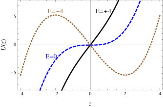
Let us consider first the unperturbed system (i.e. $p=0$). For $E>0$, the system has no equilibrium point: the particle rolls down to $-\infty$, and re-appears immediately at $+\infty$, reflecting the fact that the solution $\psi$ of the corresponding Schrödinger equation has a zero at the “time” $x$ when the particle escapes to infinity. This behaviour of the Riccati variable indicates that every $E>0$ belongs to the spectrum of the Schrödinger operator.

Equation (3.8) gives the “velocity” of the fictitious particle as a function of its position. Hence the “time” taken to go from $+\infty$ to $-\infty$ is

$$-\int_{+\infty}^{-\infty}\frac{\text{d}{z}}{z^{2}+k^{2}}=\frac{\pi}{k}\,.$$

On the other hand, the solution of the Frisch-Lloyd equation for $E>0$ and $p=0$ is the Cauchy density

(3.15) $$f(z)=\frac{N}{z^{2}+k^{2}}\;\;\text{with}\;\;N=\frac{k}{\pi}\,.$$

Therefore the normalisation constant $N$ may be interpreted as the reciprocal of the “time” that the particle takes to run through ${\mathbb{R}}$. Another equivalent interpretation is as follows: recall that, when the particle escapes to $-\infty$, it is immediately re-injected at $+\infty$ to commence a new journey through ${\mathbb{R}}$. $N$ may therefore also be viewed as the current of the fictitious particle [31], and the Rice formula

$$\lim_{z\to\pm\infty}z^{2}f(z)=N$$

can be understood as expressing a relation between the stationary distribution and a current of probability. This current equals the number of infinitudes of $z(x)$— i.e. the number of nodes of the wavefunction $\psi(x)$— per unit length. By the familiar oscillation theorem of Sturm–Liouville theory, it is therefore the same as the integrated density of states per unit length of the corresponding Schrödinger Hamiltonian.

By contrast, in the case $E=-k^{2}<0$, $k>0$, the unperturbed system has an unstable equilibrium point at $-k$, and a stable equilibrium point at $k$. Unless the particle starts from a position on the left of the unstable equilibrium, it must tend asymptotically to the stable equilibrium point. The fact that the particle cannot reach infinity more than once indicates that the spectrum lies entirely in ${\mathbb{R}}_{+}$. The solution of the Frisch–Lloyd equation is

$$f(z)=\delta(z-k)\,.$$

Let us now consider how the occurence of jumps can affect the system. For $E>0$, the jumps defined by Equation (3.9), as long as they are finite and infrequent (i.e. $p$ is small), cannot prevent the particle from visiting $-\infty$ repeatedly; the system should therefore behave in much the same way as in the unperturbed case, and we expect the density $f$ to be Cauchy-like. In particular, the interpretation of the normalisation constant in terms of a probability current remains valid because, for $z$ large enough, the deterministic part (3.8) of the evolution of the Riccati variable dominates the stochastic part (3.9). The situation for $E<0$ is more complicated. Roughly speaking, positive jumps, i.e. discontinuous increases of $z$, enable the particle to make excursions to the right of the stable equilibrium point $z=k$, but the particle can never overcome the infinite barrier and so it rolls back down towards $k$. On the other hand, negative jumps, i.e. discontinuous decreases of $z$, enable the particle to make excursions to the left of $k$. If the jump is large enough, the particle can overcome the potential barrier at $-k$ and escape to $-\infty$, raising the possibility that part of the spectrum of the Schrödinger operator lies in ${\mathbb{R}}_{-}$. For small $p$, we expect the density $f$ to be large in the neighbourhood of $z=k$.

We shall return to this useful particle analogy in later sections when we examine the detailed behaviour of the Riccati variable for specific random point scatterers.

3.4. The reduced Lyapunov exponent

Knowing the density of the invariant measure, the calculation of the Lyapunov exponent reduces, thanks to Formula (1.3), to the evaluation of a multiple integral. We will show in this subsection that, if $A$ is of the form (3.4) and the boundary matrix $B$ is triangular, then this formula may be greatly simplified. As pointed out in §3.1, there is no loss of generality in setting $E=k^{2}=1$ since the parameter $k$ may be re-introduced subsequently by rescaling. This has the advantage of making the calculation simpler.

For definiteness, let us begin with the upper triangular case, i.e. $b_{21}=0$. Then the density of the invariant measure satisfies the Frisch–Lloyd equation (3.13), again with $E=1$, and we have

(3.16) $$\left|A\begin{pmatrix}z\\ 1\end{pmatrix}\right|^{2}=\left|B\begin{pmatrix}z\\ 1\end{pmatrix}\right|^{2}=\left(b_{11}z+b_{12}\right)^{2}+\left(b_{21}z+b_{22}\right)^{2}\\ =\left(b_{21}z+b_{22}\right)^{2}\left[1+{\mathscr{B}}(z)^{2}\right]=b_{22}^{2}\left[1+{\mathscr{B}}(z)^{2}\right]\,.$$

Hence

(3.17) $$\gamma_{\mu}=\frac{1}{2}\int_{\mathbb{R}}\text{d}z\int_{\text{SL}(2,\mathbb{R})}\kappa(\text{d}B)\,\ln\frac{\left|A\begin{pmatrix}z\\ 1\end{pmatrix}\right|^{2}}{\left|\begin{pmatrix}z\\ 1\end{pmatrix}\right|^{2}}\,f(z)\\ =\frac{1}{2}\int_{\mathbb{R}}\text{d}z\int_{\text{SL}(2,\mathbb{R})}\kappa(\text{d}B)\,\ln\frac{b_{22}^{2}\left[1+{\mathscr{B}}(z)^{2}\right]}{1+z^{2}}\,f(z)$$

and, after some re-arrangement,

(3.18) $$\gamma_{\mu}={\mathbb{E}}\left(\ln|b_{22}|\right)+\frac{1}{2}\int_{\mathbb{R}}\text{d}z\int_{\text{SL}(2,\mathbb{R})}\kappa(\text{d}B)\,\ln\left[1+{\mathscr{B}}(z)^{2}\right]\,f(z)\\ -\frac{1}{2}\int_{\mathbb{R}}\text{d}z\int_{\text{SL}(2,\mathbb{R})}\kappa(\text{d}B)\,\ln(1+z^{2})\,f(z)\,.$$

Consider the second term on the right-hand side of the last equality: by changing the order of integration, and making the substitution $y={\mathscr{B}}(z)$ in the inner integral, we obtain

(3.19) $$\frac{1}{2}\int_{\mathbb{R}}\text{d}z\int_{\text{SL}(2,\mathbb{R})}\kappa(\text{d}B)\,\ln\left[1+{\mathscr{B}}(z)^{2}\right]\,f(z)\\ =\frac{1}{2}\int_{\text{SL}(2,\mathbb{R})}\kappa(\text{d}B)\,\int_{\mathbb{R}}\text{d}z\,\ln\left[1+{\mathscr{B}}(z)^{2}\right]f(z)\\ =\frac{1}{2}\int_{\text{SL}(2,\mathbb{R})}\kappa(\text{d}B)\,\int_{\mathbb{R}}\text{d}y\,\ln\left[1+y^{2}\right]f\left({\mathscr{B}}^{-1}(y)\right)\frac{\text{d}{\mathscr{B}}^{-1}}{\text{d}y}(y)\,.$$

Next, we use the letter $z$ instead of $y$, and change the order of integration again: Equation (3.18) becomes

(3.20) $$\gamma_{\mu}={\mathbb{E}}\left(\ln|b_{22}|\right)\\ +\frac{1}{2}\int_{\mathbb{R}}\,\text{d}z\int_{\text{SL}(2,\mathbb{R})}\kappa(\text{d}B)\,\left[f\left({\mathscr{B}}^{-1}(z)\right)\,\frac{\text{d}{\mathscr{B}}^{-1}}{\text{d}z}(z)-f(z)\right]\,\ln(1+z^{2})\,.$$

Finally, by making use of Equation (3.13), and then integrating by parts, we arrive at the following formula:

(3.21) $$\gamma_{\mu}=\frac{1}{p}\,\gamma$$

where

(3.22) $$\gamma:=p\,{\mathbb{E}}\left(\ln|b_{22}|\right)+\mathchoice{{\vbox{\hbox{$\textstyle-$}}\kern-4.86108pt}}{{\vbox{\hbox{$\scriptstyle-$}}\kern-3.25pt}}{{\vbox{\hbox{$\scriptscriptstyle-$}}\kern-2.29166pt}}{{\vbox{\hbox{$\scriptscriptstyle-$}}\kern-1.875pt}}\!\int_{-\infty}^{\infty}\text{d}z\,zf(z)\,,\quad b_{21}=0\,.$$

This formula remains unchanged after restoring $k$ by rescaling. A similar calculation may be carried out if, instead, $B$ is lower triangular. Equation (3.21) then holds with

(3.23) $$\gamma:=p\,{\mathbb{E}}\left(\ln|b_{11}|\right)-\mathchoice{{\vbox{\hbox{$\textstyle-$}}\kern-4.86108pt}}{{\vbox{\hbox{$\scriptstyle-$}}\kern-3.25pt}}{{\vbox{\hbox{$\scriptscriptstyle-$}}\kern-2.29166pt}}{{\vbox{\hbox{$\scriptscriptstyle-$}}\kern-1.875pt}}\!\int_{-\infty}^{\infty}\text{d}z\,\frac{E}{z}f(z)\,,\quad b_{12}=0\,.$$

The integrals in these expressions are Cauchy principal value integrals.

We shall henceforth refer to $\gamma$ as the reduced Lyapunov exponent. Although our derivation of the relation between $\gamma_{\mu}$ and $\gamma$ assumed that $E>0$, we conjecture, on the basis of the numerical evidence obtained in all the examples we considered, that it holds also when $E<0$.

Such simplified formulae for the Lyapunov exponent are well-known in the physics literature [31]. The reduced Lyapunov exponent is the rate of growth of the solution of the Schrödinger equation:

$$\gamma=\lim_{x\rightarrow\infty}\frac{1}{x}\ln\sqrt{\psi(x)^{2}+\left[\psi^{\prime}(x)\right]^{2}}\,.$$

Alternatively, using the stationarity of the process $\{z(x)\}$,

$$\gamma=\lim_{x\rightarrow\infty}\frac{1}{x}\ln\left|\psi(x)\right|+\lim_{x\rightarrow\infty}\frac{1}{x}\ln\sqrt{1+z^{2}(x)}=\lim_{x\rightarrow\infty}\frac{1}{x}\ln\left|\psi(x)\right|$$

and

$$\gamma=\lim_{x\rightarrow\infty}\frac{1}{x}\ln\left|\psi^{\prime}(x)\right|+\lim_{x\rightarrow\infty}\frac{1}{x}\ln\sqrt{1/z^{2}(x)+1}=\lim_{x\rightarrow\infty}\frac{1}{x}\ln\left|\psi^{\prime}(x)\right|\,.$$

$\gamma$ also provides a reasonable definition of (the reciprocal of) the localisation length of the system.

The presence of the expectation term on the right-hand side of Equation (3.22) may, at first sight, surprise readers familiar with the case of delta scatterers, but its occurence in our more general context is easily explained as follows: between consecutive scatterers, the wave function is continuous and so, for $x_{n}<x<x_{n+1}$, we can write

(3.24) $$\ln|\psi(x)|=\ln|\psi(x_{n}+)|+\int_{x_{n}}^{x}\text{d}y\,\frac{\text{d}}{\text{d}y}\ln|\psi(y)|\\ =\ln|\psi(x_{n}+)|+\int_{x_{n}}^{x}\text{d}y\,z(y)\,.$$

Let us denote by $b_{ij}^{(n)}$ the entry of $B_{n}$ in the $i$th row and $j$th column. If $B$ is upper triangular, we have, at $x_{n}$,

$$\psi(x_{n}+)=b_{22}^{(n)}\,\psi(x_{n}-)$$

and so the wavefunction is discontinuous there unless $b_{22}^{(n)}=1$. Reporting this in (3.24) and iterating, we obtain

$$\ln|\psi(x)|=\ln|\psi(0)|+\sum_{j=1}^{n(x)}\ln\left|b_{22}^{(j)}\right|+\int_{0}^{x}\text{d}y\,z(y)$$

where $n(x)$, as defined in §3.2, is the number of point scatterers in the interval $[0,x]$. Using

$${\mathbb{E}}(n(x))=px$$

and the ergodicity of the Riccati variable, we recover by this other route the equation (3.22) obtained earlier. It is now clear that the expectation term arises from the possible discontinuities of the wave function at the scatterers. To give two examples: for the delta scatterer, the wave function is continuous everywhere, $b_{22}=1$ and so Equation (3.22) is just the familiar formula in [31]. For the supersymmetric scatterer, however, the wavefunction has discontinuites,

$$b_{22}=\text{e}^{-w}$$

and so, as noted in [41], the formula for the reduced Lyapunov exponent must include the additional term

$${\mathbb{E}}\left(\ln|b_{22}|\right)=-{\mathbb{E}}(w)\,.$$

If $B$ is lower triangular instead, it is more natural to work with $\psi^{\prime}$: for $x_{n}<x<x_{n+1}$, we have

(3.25) $$\ln|\psi^{\prime}(x)|=\ln|\psi^{\prime}(x_{n}+)|+\int_{x_{n}}^{x}\text{d}y\,\frac{\text{d}}{\text{d}y}\ln|\psi^{\prime}(y)|\\ =\ln|\psi^{\prime}(x_{n}+)|+\int_{x_{n}}^{x}\frac{\psi^{\prime\prime}(y)}{\psi^{\prime}(y)}\,\text{d}y=\ln|\psi^{\prime}(x_{n}+)|-k^{2}\int_{x_{n}}^{x}\frac{\psi(y)}{\psi^{\prime}(y)}\,\text{d}y\\ =\ln|\psi^{\prime}(x_{n}+)|-k^{2}\int_{x_{n}}^{x}\text{d}y\,\frac{1}{z(y)}\,.$$

Using the lower triangularity of $B_{n}$, we obtain, at $x_{n}$,

$$\psi^{\prime}(x_{n}+)=b_{11}^{(n)}\,\psi^{\prime}(x_{n}-)\,.$$

By repeating our earlier argument, we recover Equation (3.23).

3.5. Halperin’s trick and the energy parameter

For the particular case of delta scatterers, Halperin [25] devised an ingenious method that, at least in some cases, by-passes the need for quadrature and yields analytical expressions for the reduced Lyapunov exponent. Let us give a brief outline of Halperin’s trick and discuss some of its consequences.

Halperin works with the Fourier transform of the invariant density:

(3.26) $$F(x):=\int_{\mathbb{R}}f(z)\,\text{e}^{-\text{i}xz}\,\text{d}z\,.$$

For the delta scatterer, the Frisch–Lloyd equation (3.14) in Fourier space is then

(3.27) $$F^{\prime\prime}(x)-E\,F(x)-p\,\frac{{\mathbb{E}}\left(\text{e}^{-\text{i}xu}\right)-1}{\text{i}x}\,F(x)=-2\pi\,N\,\delta(x)\,.$$

Let $\varepsilon>0$ and integrate over the interval $(-\varepsilon,\varepsilon)$. Using the fact that

$$F^{\prime}(-\varepsilon)=-\overline{F^{\prime}(\varepsilon)}$$

and letting $\varepsilon\rightarrow 0+$, we obtain

$$N=-\frac{1}{\pi}\text{Re}\left[F^{\prime}(0+)\right]\>.$$

Furthermore, since in this case $b_{11}=1$ and $b_{21}=0$, Equation (3.22) leads to

$$\gamma=\mathchoice{{\vbox{\hbox{$\textstyle-$}}\kern-4.86108pt}}{{\vbox{\hbox{$\scriptstyle-$}}\kern-3.25pt}}{{\vbox{\hbox{$\scriptscriptstyle-$}}\kern-2.29166pt}}{{\vbox{\hbox{$\scriptscriptstyle-$}}\kern-1.875pt}}\!\int_{-\infty}^{\infty}z\,f(z)\,\text{d}z=-\text{Im}\left[F^{\prime}(0+)\right]\,.$$

These two formulae may be combined neatly by introducing the so-called characteristic function $\Omega$ associated with the system [32, 34]:

(3.28) $$\Omega(E):=\gamma(E)-\text{i}\pi N(E)\,.$$

Then Halperin observes that

(3.29) $$\Omega(E)=\text{i}\frac{F^{\prime}(0+)}{F(0+)}$$

where, with a slight abuse of notation, $F$ is now the particular solution of the homogeneous version of Equation (3.27) satisfying the condition

$$\lim_{x\rightarrow+\infty}F(x)=0\,.$$

Thus the problem of evaluating $\gamma$ and $N$ has been reduced to that of finding the recessive solution of a linear homogeneous differential equation.

Equation (3.29) expresses a relationship between the density of states and the Lyapunov exponent— a relationship made more explicit in the Herbert–Jones–Thouless formula [26, 42] well-known in the theory of quantum disordered systems. A further consequence of the same equation is that, if the recessive solution $F$ depends analytically on the energy parameter, so does the characteristic function. $\Omega$ should thus have an analytic continuation everywhere in the complex plane, save on the cut where the essential spectrum of the Schrödinger Hamiltonian lies.

More generally, for an arbitrary scatterer, the Fourier transform $F$ of the invariant density satisfies the equation

(3.30) $$F^{\prime\prime}(x)-E\,F(x)-p\int_{\text{SL}(2,\mathbb{R})}\kappa(\text{d}B)\int_{\mathbb{R}}\text{d}z\,\frac{\text{e}^{-\text{i}x{\mathscr{B}}(z)}-\text{e}^{-\text{i}xz}}{\text{i}x}\,f(z)=0\,.$$

We shall not make explicit use of this equation in what follows: instead, we shall obtain closed formulae for the characteristic function by making use of analytic continuation. This is one important benefit of having retained the energy parameter.

3.6. Random continued fractions

There is a close correspondence between products of $2\times 2$ matrices and continued fractions. Let $z_{0}$ be an arbitrary starting value, recall the definition (1.4) and set

(3.31) $$z_{n}:={\mathscr{A}}_{n-1}\circ\cdots\circ{\mathscr{A}}_{0}(z_{0})\,.$$

Then the sequence $\{z_{n}\}_{n\in{\mathbb{N}}}$ is a Markov chain on the projective line, and $\nu$ is $\mu$-invariant if and only if it is a stationary distribution of this Markov chain. Now, reverse the order of the matrices in the product, set $\zeta_{0}=z_{0}$ and

(3.32) $$\zeta_{n}:={\mathscr{A}}_{0}\circ\cdots\circ{\mathscr{A}}_{n-1}(\zeta_{0})\,.$$

Although, for every $n$, $z_{n}$ and $\zeta_{n}$ have the same distribution, the large-$n$ behaviour of a typical realisation of the sequence $\{z_{n}\}_{n\in{\mathbb{N}}}$ differs greatly from that of a typical realisation of the sequence $\{\zeta_{n}\}_{n\in{\mathbb{N}}}$ [20].

$\{\zeta_{n}\}_{n\in{\mathbb{N}}}$ converges to a (random) limit, say $\zeta$. Write

$$A_{n}:=\begin{pmatrix}a_{n}&b_{n}\\ c_{n}&d_{n}\end{pmatrix}\,.$$

Then

(3.33) $${\mathscr{A}}_{n}(\zeta)=a_{n}/c_{n}-\frac{1/c_{n}^{2}}{d_{n}/c_{n}+\zeta}$$

and so

(3.34) $$\zeta:=a_{0}/c_{0}-\cfrac{1/c_{0}^{2}}{d_{0}/c_{0}+a_{1}/c_{1}-\cfrac{1/c_{1}^{2}}{d_{1}/c_{1}+a_{2}/c_{2}-\cfrac{1/c_{2}^{2}}{d_{2}/c_{2}+\cdots}}}\,.$$

It is immediately clear that, if $A$ is $\mu$-distributed, then

$${\mathscr{A}}(\zeta)=a/c-\frac{1/c^{2}}{d/c+\zeta}$$

has the same distribution as $\zeta$. Hence the distribution of $\zeta$ is $\mu$-invariant. Furthermore, if $\zeta$ is independent of $z_{0}$, then there can be only one $\mu$-invariant measure. So $f$ is also the density of the infinite random continued fraction $\zeta$.

By contrast, $\{z_{n}\}_{n\in{\mathbb{N}}}$ behaves ergodically. Therefore the density $f$ of the invariant measure $\nu$ should be well approximated by a histogram of the $z_{n}$. We have used this to verify the correctness of our results.

4. Some explicit invariant measures

4.1. Delta scatterers

In this section, we obtain invariant measures for products where the matrices are of the form

(4.1) $$A=\begin{pmatrix}\sqrt{k}&0\\ 0&\frac{1}{\sqrt{k}}\end{pmatrix}\begin{pmatrix}\cos(k\theta)&-\sin(k\theta)\\ \sin(k\theta)&\cos(k\theta)\end{pmatrix}\begin{pmatrix}\frac{1}{\sqrt{k}}&0\\ 0&\sqrt{k}\end{pmatrix}\begin{pmatrix}1&u\\ 0&1\end{pmatrix}$$

or

(4.2) $$A=\begin{pmatrix}\sqrt{k}&0\\ 0&\frac{1}{\sqrt{k}}\end{pmatrix}\begin{pmatrix}\cosh(k\theta)&\sinh(k\theta)\\ \sinh(k\theta)&\cosh(k\theta)\end{pmatrix}\begin{pmatrix}\frac{1}{\sqrt{k}}&0\\ 0&\sqrt{k}\end{pmatrix}\begin{pmatrix}1&u\\ 0&1\end{pmatrix}$$

where $\theta\sim\text{Exp}(p)$ and $u$ is a random variable, independent of $\theta$, whose density we denote by $\varrho:{\mathbb{R}}\rightarrow{\mathbb{R}}_{+}$. These products are associated with the generalised Kronig–Penney model for $E=k^{2}>0$ and $E=-k^{2}$ respectively, in the case where (see Example 1)

$$B=\begin{pmatrix}1&u\\ 0&1\end{pmatrix}\,.$$

The corresponding Frisch–Lloyd equation (3.14) is

$$(z^{2}+E)\,f(z)+p\int_{\mathbb{R}}\text{d}u\int_{z}^{z-u}\text{d}t\,f(t)\,\varrho(u)=N\,.$$

We change the order of integration; the equation becomes

(4.3) $$N=(z^{2}+E)\,f(z)+p\int_{\mathbb{R}}\text{d}t\,K(z-t)\,f(t)$$

where

(4.4) $$K(x)=\begin{cases}-\int_{x}^{\infty}\varrho(u)\,\text{d}u&\text{if $x>0$}\\ \int_{-\infty}^{x}\varrho(u)\,\text{d}u&\text{if $x<0$}\end{cases}\,.$$

Suppose that

(4.5) $$\pm u\sim\text{\tt Exp}(q)\,.$$

We shall show that, in this case, the Frisch–Lloyd equation reduces to a first-order differential equation. For the sake of clarity, consider first the case $u\sim\text{Exp}(q)$. For this choice of distribution,

$$K(x)=\begin{cases}-\text{e}^{-qx}&\text{if $x>0$}\\ 0&\text{if $x<0$}\end{cases}\,.$$

So we have

$$K^{\prime}(x)=-qK(x)\,,\;\;K(0+)=-1\,,$$

and equation (4.3) is

$$N=(z^{2}+E)\,f(z)+p\int_{-\infty}^{z}\text{d}t\,K(z-t)\,f(t)\,.$$

Differentiate this equation with respect to $z$:

(4.6) $$0=\frac{\text{d}}{\text{d}z}\left[(z^{2}+E)\,f(z)\right]+pK(0+)f(z)+p\int_{-\infty}^{z}\text{d}t\,K^{\prime}(z-t)\,f(t)\\ =\frac{\text{d}}{\text{d}z}\left[(z^{2}+E)\,f(z)\right]-pf(z)-qp\int_{-\infty}^{z}\text{d}t\,K(z-t)\,f(t)\\ =\frac{\text{d}}{\text{d}z}\left[(z^{2}+E)\,f(z)\right]-pf(z)-q\left[N-(z^{2}+E)\,f(z)\right]\,.$$

This is the required differential equation. The case $-u\sim\text{Exp}(q)$ is analogous, and so we find, for the general case (4.5),

(4.7) $$\frac{\text{d}}{\text{d}z}\left[(z^{2}+E)\,f(z)\right]-p\,f(z)\pm q\left[(z^{2}+E)\,f(z)\right]=\pm qN\,.$$

We seek the particular solution that satisfies the normalisation condition

(4.8) $$\int_{\mathbb{R}}f(z)\,\text{d}z=1\,.$$

This condition fixes the constant of integration $N$, and hence provides an expression for the integrated density of states for the Schrödinger Hamiltonian.

4.1.1. Product of the form (4.1)

For $E=k^{2}>0$, this leads to

(4.9) $$f(z)=\frac{\pm qN}{z^{2}+k^{2}}\exp\left[\mp qz+\frac{p}{k}\arctan\frac{z}{k}\right]\\ \times\int_{\mp\infty}^{z}\exp\left[\pm qt-\frac{p}{k}\arctan\frac{t}{k}\right]\,\text{d}t\,.$$

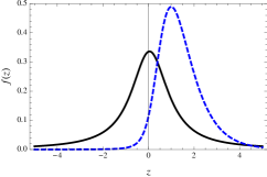
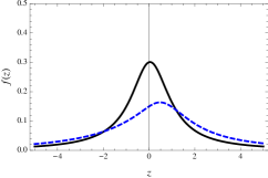
The density of the Riccati variable is plotted in Figure 3 for (a) positive $u_{n}$ and (b) negative $u_{n}$. The continuous black curves correspond to a low density of scatterers (small $p$, compared to $k$ and $1/q$) and are reminiscent of the Cauchy law obtained in the absence of scatterers. Recall that the effect of the $n$th scatterer on the Riccati variable is described by the equation

$$z(x_{n}+)=z(x_{n}-)+u_{n}\,.$$

When the $u_{n}$ are positive, any increase in the concentration of the scatterers produces a decrease in the current and so the distribution is pushed to the right; see the blue dashed curve in Figure 3 (a). On the other hand, when the $u_{n}$ are negative, any increase in the concentration of the scatterers leads to an increase in the current of the Riccati variable and so spreads the distribution; see the blue dashed curve in Figure 3 (b).

Figure 3. Plots of the invariant density $f$ for delta scatterers and positive energy $E=k^{2}=+1$. Black continuous lines correspond to a low density of scatterers, i.e. $\theta\sim{\tt Exp}(p)$ with $p=1/4$, and blue dashed lines to a high density, i.e. $p=4$. (a) $u\sim\text{\tt Exp}(1)$; (b) $-u\sim\text{\tt Exp}(1)$.

4.1.2. Product of the form (4.2)

For $E=-k^{2}<0$ and $u\sim\text{Exp}(q)$, one must take $N=0$ to obtain a normalisable solution— a reflection of the fact that the essential spectrum of the Schrödinger Hamiltonian is ${\mathbb{R}}_{+}$. Then

(4.10) $$f(z)=C^{-1}\frac{\text{e}^{-qz}}{z^{2}-k^{2}}\left(\frac{z-k}{z+k}\right)^{\frac{p}{2k}}{\mathbf{1}}_{(k,\infty)}(z)$$

where $C$ is the normalisation constant.

By contrast, in the case $-u\sim\text{\tt Exp}(q)$, one finds

(4.11) $$f(z)=\frac{qN}{z^{2}-k^{2}}\text{e}^{qz}\left|\frac{z-k}{z+k}\right|^{\frac{p}{2k}}\int_{z}^{c(z)}\text{e}^{-qt}\left|\frac{t+k}{t-k}\right|^{\frac{p}{2k}}\,\text{d}t$$

where

$$c(z)=\begin{cases}\infty&\text{if $z>k$}\\ -k&\text{if $z<k$}\end{cases}\>.$$

Figure 4. Plots of the invariant density $f$ for delta scatterers and negative energy $E=-k^{2}=-1$. Black continuous lines correspond to a “low” density of scatterers, i.e. $\theta\sim{\tt Exp}(p)$ with $p=1/4$, and blue dashed lines to a “high” density $p=4$. (a) $u\sim\text{\tt Exp}(1)$; (b) $-u\sim\text{\tt Exp}(1)$.

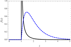
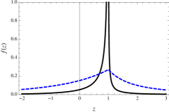
The invariant density $f$ is plotted in Figure 4 for the cases (a) $u\sim{\tt Exp}(q)$ and (b) $-u\sim{\tt Exp}(q)$ respectively. The shape of the distribution can again be explained by using the qualitative picture of §3.3. For positive $u_{n}$, the sharp peak obtained for a small concentration $p$ of scatterers (black continuous line) reflects the trapping of the process $\{z(x)\}$ by the potential well at $z=k$; recall Figure 2. When the concentration of scatterers is increased, the Riccati variable experiences positive jumps more frequently and so the distribution spreads to the right (blue dashed curve). For negative $u_{n}$, the jumps can take arbitrary negative values. This enables the “particle” to overcome the barrier at $z=-k$, and so we have a non-zero current $N$ (i.e. a non-zero density of states). This effect is enhanced as the density of the scatterers is increased (blue dashed curve).

4.1.3. Calculation of the characteristic function

Using the invariant measure, it is trivial to express the integrated density of states and the Lyapunov exponent in integral form. Such integral expressions are particularly useful when studying the asymptotics of $N$ and $\gamma$ in various limits. Even so, it is worth seeking analytical expressions (in terms of special functions) for these quantities, as they sometimes reveal unexpected connections to other problems.

Recalling the discussion in §3.5, we begin with a straightforward application of Halperin’s trick. For $\pm u\sim{\tt Exp}(q)$, we have

$${\mathbb{E}}\left(\text{e}^{-\text{i}ux}\right)=\frac{1}{1\pm\text{i}x/q}$$

and so the homogeneous version of Equation (3.27) is

$$F^{\prime\prime}(x)+\left[-E+\frac{p}{\pm q+\text{i}x}\right]\,F(x)=0\,.$$

The recessive solution is

$$F(x)=\frac{W_{\frac{-p}{2\sqrt{-E}},\frac{1}{2}}\left(2\sqrt{-E}\left[\text{i}x\pm q\right]\right)}{W_{\frac{-p}{2\sqrt{-E}},\frac{1}{2}}\left(\pm 2\sqrt{-E}q\right)}$$

where $W_{a,b}$ is the Whittaker function [1, 23]. We deduce that, for $E$ outside the essential spectrum of the Schrödinger Hamiltonian,

(4.12) $$\Omega(E):=\gamma(E)-\text{i}\pi N(E)=-2\sqrt{-E}\,\frac{W_{\frac{-p}{2\sqrt{-E}},\frac{1}{2}}^{\prime}\left(\pm 2\sqrt{-E}q\right)}{W_{\frac{-p}{2\sqrt{-E}},\frac{1}{2}}\left(\pm 2\sqrt{-E}q\right)}\,.$$

This formula for the characteristic function was discovered by Nieuwenhuizen [35]. In particular, for $k$ real,

$$\gamma(k^{2})-\text{i}\pi N(k^{2})=\Omega(k^{2}+\text{i}0+)=2\text{i}k\frac{W_{\frac{-\text{i}p}{2k},\frac{1}{2}}^{\prime}\left(\mp 2\text{i}kq\right)}{W_{\frac{-\text{i}p}{2k},\frac{1}{2}}\left(\mp 2\text{i}kq\right)}$$

and

$$\gamma(-k^{2})-\text{i}\pi N(-k^{2})=\Omega(-k^{2}+\text{i}0+)=-2k\frac{W_{\frac{-p}{2k},\frac{1}{2}}^{\prime}\left(\pm 2kq\right)}{W_{\frac{-p}{2k},\frac{1}{2}}\left(\pm 2kq\right)}\,.$$

In the case $u\sim{\tt Exp}(q)$ there is an alternative derivation of this formula which does not require the solution of a differential equation: start with the explicit form of the invariant density $f$ for $E=-k^{2}<0$, given by Equation (4.10). By using Formula 3 in [23], §3.384, we obtain the following expression for the normalisation constant:

$$C:=\int_{k}^{\infty}\frac{\text{e}^{-qz}}{z^{2}-k^{2}}\left(\frac{z-k}{z+k}\right)^{\frac{p}{2k}}\,\text{d}z=\frac{1}{2k}\Gamma\left(\frac{p}{2k}\right)\,W_{\frac{-p}{2k},\frac{1}{2}}\left(2kq\right)\,.$$

The reduced Lyapunov exponent $\gamma$ may then be obtained easily by noticing that differentiation with respect to the parameter $q$ yields an additional factor of $z$ in the integrand. Hence, for $k$ real, we find

$$\gamma(-k^{2})=\int_{k}^{\infty}\text{d}z\,z\,f(z)=-\frac{\partial}{\partial q}\ln C=-2k\,\frac{W^{\prime}_{\frac{-p}{2k},\frac{1}{2}}\left(2kq\right)}{W_{\frac{-p}{2k},\frac{1}{2}}\left(2kq\right)}\,.$$

Since $N=0$ for $E<0$, this yields

(4.13) $$\Omega(-k^{2})=-2k\,\frac{W^{\prime}_{\frac{-p}{2k},\frac{1}{2}}\left(2kq\right)}{W_{\frac{-p}{2k},\frac{1}{2}}\left(2kq\right)}\,.$$

Now, the half-line $E<0$ lies outside the essential spectrum of the Schrödinger Hamiltonian because $N=0$ along it. Hence $\Omega$ is analytic along this half-line, and we see that the “$+$ case” of our earlier Equation (4.12) is simply the analytic continuation of Equation (4.13). In particular, the formula in the case $E=k^{2}>0$ may be deduced from the formula in the case $E=-k^{2}<0$ by applying the simple substitution

$$k\mapsto-\text{i}k\,.$$

4.2. Delta–prime scatterers

Products of matrices of the form

(4.14) $$A=\begin{pmatrix}\sqrt{k}&0\\ 0&\frac{1}{\sqrt{k}}\end{pmatrix}\begin{pmatrix}\cos(k\theta)&-\sin(k\theta)\\ \sin(k\theta)&\cos(k\theta)\end{pmatrix}\begin{pmatrix}\frac{1}{\sqrt{k}}&0\\ 0&\sqrt{k}\end{pmatrix}\begin{pmatrix}1&0\\ v&1\end{pmatrix}$$

or

(4.15) $$A=\begin{pmatrix}\sqrt{k}&0\\ 0&\frac{1}{\sqrt{k}}\end{pmatrix}\begin{pmatrix}\cosh(k\theta)&\sinh(k\theta)\\ \sinh(k\theta)&\cosh(k\theta)\end{pmatrix}\begin{pmatrix}\frac{1}{\sqrt{k}}&0\\ 0&\sqrt{k}\end{pmatrix}\begin{pmatrix}1&0\\ v&1\end{pmatrix}$$

where $\theta\sim\text{Exp}(p)$ and $v$ is a random variable independent of $\theta$, are associated with the delta-prime scatterer (see Example 2)

$$B=\begin{pmatrix}1&0\\ v&1\end{pmatrix}\,.$$

The Frisch–Lloyd equation (3.14) for this scatterer is

(4.16) $$(z^{2}+E)\,f(z)+p\int_{\mathbb{R}}\text{d}v\int_{z}^{\frac{z}{1-vz}}\text{d}t\,f(t)\,\varrho(v)=N$$

where $\varrho$ is the density of $v$. The calculation of the invariant measure in this case can be reduced to the calculation of the invariant measure for some Kronig–Penney model with delta scatterers. For instance, in the negative energy case (4.15) with $k=1$, we have

$$\begin{pmatrix}0&1\\ 1&0\end{pmatrix}A\begin{pmatrix}0&1\\ 1&0\end{pmatrix}=\begin{pmatrix}\cosh\theta&\sinh\theta\\ \sinh\theta&\cosh\theta\end{pmatrix}\begin{pmatrix}1&v\\ 0&1\end{pmatrix}\,.$$

The similarity transformation of the matrix $A$ on the left corresponds to the transformation $z\mapsto 1/z$ of the Riccati variable. So the invariant densities for the delta and the delta-prime cases are in a reciprocal relationship. Accordingly, replace $z$ by $1/z$ in Equation (4.16) and set

$$g(z)=\frac{1}{z^{2}}f(1/z)\,.$$

Then

(4.17) $$N=\left(1+Ez^{2}\right)g(z)-p\int_{\mathbb{R}}\text{d}v\int_{z}^{z-v}\text{d}t\,g(t)\,\varrho(v)\\ =\left(1+Ez^{2}\right)g(z)-p\int_{\mathbb{R}}\text{d}t\,K(z-t)\,g(t)$$

where $K$ is the kernel defined by Equation (4.4). This equation for $g$ is essentially the same as Equation (4.3) save for the sign of $p$ and the dependence on the energy. For the case

$$\pm v\sim{\tt Exp}(q)$$

this equation can, by using the same tricks as before, be converted into a differential equation which is easy to solve.

4.2.1. Product of the form (4.14)

For $E=k^{2}>0$, the upshot is

(4.18) $$f(z)=\frac{\pm qN}{z^{2}+k^{2}}\exp\left[\mp\frac{q}{z}-\frac{p}{k}\arctan\frac{k}{z}\right]\\ \times\int_{\mp\infty}^{1/z}\exp\left[\pm qt+\frac{p}{k}\arctan(kt)\right]\,\text{d}t\,.$$

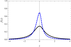
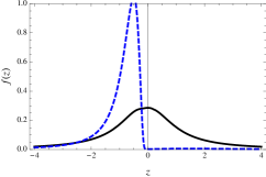
Plots of the distribution are shown in Figure 5 for (a) positive $v_{n}$ and (b) negative $v_{n}$. These plots differ somewhat from those obtained in the case of delta scatterers, and we can use the particle analogy of §3.3 to explain the differences. The jump of the particle associated with the $n$th delta-prime scatterer is given implicitly by

(4.19) $$\frac{1}{z(x_{n}+)}=\frac{1}{z(x_{n}-)}+v_{n}\,.$$

The strongly asymmetric distribution obtained for negative $v_{n}$ (Part (b) of Figure 5) can be explained as follows: starting from $+\infty$, the particle experiences its first jump at “time” $x_{1}$, and its value after the jump is approximately $1/v_{1}<0$. In fact, for $z$ negative and small in modulus, the invariant density resembles very closely that of $1/v_{1}$, i.e.

$$f(z)\sim\frac{c}{z^{2}}\text{e}^{q/z}\;\;\text{as $z\rightarrow 0-$}\,.$$

Thereafter, the particle proceeds towards $-\infty$. In particular, if $p$ is large, then the expected value of $x_{1}$ is small, and the particle spends hardly any time on the positive semi-axis.

Figure 5. Plots of the invariant density $f$ for delta-prime scatterers and positive energy $E=k^{2}=+1$. Black continuous lines correspond to a “low” density of scatterers, i.e. $\theta\sim{\tt Exp}(p)$ with $p=1/4$, and blue dashed lines to a “high” density $p=4$. (a) $v\sim\text{\tt Exp}(1)$. (b) $-v\sim\text{\tt Exp}(1)$.

Product of the form (4.15): for $E=-k^{2}<0$ and $v\sim\text{\tt Exp}(q)$, we find

(4.20) $$f(z)=C^{-1}\,\frac{\text{e}^{-q/z}}{k^{2}-z^{2}}\left(\frac{k-z}{k+z}\right)^{\frac{p}{2k}}\,{\mathbf{1}}_{(0,k)}(z)$$

where

(4.21) $$C=\frac{1}{2k}\Gamma\left(\frac{p}{2k}\right)W_{-\frac{p}{2k},\frac{1}{2}}\left(2q/k\right)\,.$$

When $E=-k^{2}<0$ and $-v\sim\text{\tt Exp}(q)$, we obtain

(4.22) $$f(z)=\frac{qN}{z^{2}-k^{2}}\text{e}^{q/z}\left|\frac{z-k}{z+k}\right|^{\frac{p}{2k}}\int_{c(z)}^{1/z}\text{e}^{-qt}\left|\frac{1+kt}{1-kt}\right|^{\frac{p}{2k}}\,\text{d}t$$

where

$$c(z)=\begin{cases}\infty&\text{if $0<z<1/k$}\\ -k&\text{otherwise}\end{cases}\,.$$

Figure 6. Plots of the invariant density $f$ for delta-prime scatterers and negative energy $E=-k^{2}=-1$. Black continuous lines correspond to a “low” density of scatterers, i.e. $\theta\sim{\tt Exp}(p)$ with $p=1/4$, and blue dashed lines to a “high” density $p=4$. (a) $v\sim\text{\tt Exp}(1)$. (b) $-v\sim\text{\tt Exp}(1)$.

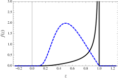
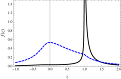
Again, we can try to understand the qualitative features of the density function $f$ for $E<0$ by invoking the particle analogy of §3.3. In view of Equation (4.19), when $v_{n}\sim{\tt Exp}(q)$ and $z(x_{n}-)>0$, the value of the Riccati variable decreases but can never become negative. So the particle, once it passes to the left of the equilibrium point at $z=k$, must remain trapped there. This explains why the density is supported on $(0,k)$; see Figure 6 (a). By contrast, when $-v_{n}\sim{\tt Exp}(q)$, the jumps are unrestricted; the “particle” can escape over the potential barrier at $z=-k$ infinitely often, leading to a non-zero current and a density $f$ spread over ${\mathbb{R}}$. This is shown in Figure 6 (b).

4.2.2. Calculation of the characteristic function

We begin with the case $v\sim{\tt Exp}(q)$ and $E=-k^{2}<0$.

The invariant density is then given by Equation (4.20). Using Formula (3.23) for the reduced Lyapunov exponent and the expression (4.21) for the normalisation constant $C$, we find

$$\gamma(-k^{2})=-k^{2}\frac{\partial}{\partial q}\ln C=-2k\frac{W_{\frac{-p}{2k},\frac{1}{2}}^{\prime}\left(2q/k\right)}{W_{\frac{-p}{2k},\frac{1}{2}}\left(2q/k\right)}\,.$$

Since $N(-k^{2})=0$ in this case, analytic continuation yields

(4.23) $$\Omega(E)=-2\sqrt{-E}\,\frac{W_{\frac{-p}{2\sqrt{-E}},\frac{1}{2}}^{\prime}\left(2q/\sqrt{-E}\right)}{W_{\frac{-p}{2\sqrt{-E}},\frac{1}{2}}\left(2q/\sqrt{-E}\right)}\,.$$

The characteristic function in the case $-v\sim{\tt Exp}(q)$ is the same, except that $q$ becomes $-q$. In particular, for $E=k^{2}>0$ and $\pm v\sim{\tt Exp}(q)$, we obtain

$$\gamma(k^{2})-\text{i}\pi N(k^{2})=\Omega(k^{2}+\text{i}0+)=2\text{i}k\frac{W_{\frac{-\text{i}p}{2k},\frac{1}{2}}^{\prime}\left(\pm 2\text{i}q/k\right)}{W_{\frac{-\text{i}p}{2k},\frac{1}{2}}\left(\pm 2\text{i}q/k\right)}\,.$$

An alternative derivation of these results could use the correspondence between the delta and delta-prime cases alluded to earlier.

4.3. Supersymmetric scatterers

We now consider products where the matrices are of the form

(4.24) $$A=\begin{pmatrix}\sqrt{k}&0\\ 0&\frac{1}{\sqrt{k}}\end{pmatrix}\begin{pmatrix}\cos(k\theta)&-\sin(k\theta)\\ \sin(k\theta)&\cos(k\theta)\end{pmatrix}\begin{pmatrix}\frac{1}{\sqrt{k}}&0\\ 0&\sqrt{k}\end{pmatrix}\begin{pmatrix}\text{e}^{w}&0\\ 0&\text{e}^{-w}\end{pmatrix}$$

or

(4.25) $$A=\begin{pmatrix}\sqrt{k}&0\\ 0&\frac{1}{\sqrt{k}}\end{pmatrix}\begin{pmatrix}\cosh(k\theta)&\sinh(k\theta)\\ \sinh(k\theta)&\cosh(k\theta)\end{pmatrix}\begin{pmatrix}\frac{1}{\sqrt{k}}&0\\ 0&\sqrt{k}\end{pmatrix}\begin{pmatrix}\text{e}^{w}&0\\ 0&\text{e}^{-w}\end{pmatrix}$$

where $\theta\sim\text{Exp}(p)$ and $w$ is a random variable independent of $\theta$. These products arise in the solution of the generalised Kronig–Penney model with the supersymmetric interaction of Example 3, i.e.

$$B=\begin{pmatrix}\text{e}^{w}&0\\ 0&\text{e}^{-w}\end{pmatrix}\,.$$

Let $\varrho$ denote the density of $w$. The Frisch–Lloyd equation (3.14) is

$$(z^{2}+E)\,f(z)+p\int_{\mathbb{R}}\text{d}w\int_{z}^{z\text{e}^{-2w}}\text{d}t\,f(t)\,\varrho(w)=N\,.$$

After changing the order of integration, this becomes

(4.26) $$N=(z^{2}+E)\,f(z)+p\int_{0}^{\infty}K\left(\frac{1}{2}\ln\frac{z}{t}\right)\,f(t)\,\text{d}t$$

where $K$ is the kernel defined by Equation (4.4).

Let

$$\pm w\sim\text{\tt Exp}(q)\,.$$

Then the kernel is supported on ${\mathbb{R}}_{\pm}$ and satisfies the differential equation

$$K^{\prime}(x)=\mp qK(x)\,,\;\;K(0\pm)=\mp 1\,.$$

We deduce

(4.27) $$\frac{\text{d}}{\text{d}z}\left[(z^{2}+E)\,f(z)\right]-p\,f(z)\pm q\frac{z^{2}+E}{2z}\,f(z)=\pm\frac{q}{2z}\,N$$

where $N$ is the integrated density of states.

Before going on to solve this equation, let us make a general remark: in the supersymmetric case, if one knows the invariant density, say $f_{+}$, for a certain distribution of the strength $w$, then one can easily deduce the invariant density, say $f_{-}$, when the sign of the strength is reversed. For instance, in the case $E=1$, the relationship between $f_{-}$ and $f_{+}$ is simply

$$f_{-}(z)=\frac{1}{z^{2}}f_{+}\left(-\frac{1}{z}\right)\,.$$

This relationship can be deduced directly from the form of the matrices in the product (4.24). It is also connected with the fact that changing the sign of the superpotential $W$ in Example 3 corresponds to swapping the functions $\phi$ and $\psi$— a manifestation of the so-called supersymmetry of the Hamiltonian.

4.3.1. Product of the form (4.24).

For $E=k^{2}>0$ and $\pm w\sim{\tt Exp}(q)$, we have

(4.28) $$f(z)=N\frac{\mp\frac{q}{2}|z|^{\mp\frac{q}{2}}}{z^{2}+k^{2}}\exp\left[\frac{p}{k}\arctan\frac{z}{k}\right]\\ \times\int_{z}^{c_{\pm}(z)}|t|^{\pm\frac{q}{2}}\exp\left[-\frac{p}{k}\arctan\frac{t}{k}\right]\frac{\text{d}t}{t}$$

where

$$c_{+}(z)=0\;\;\text{and}\;\;c_{-}(z)=\begin{cases}\infty&\text{if $z>0$}\\ -\infty&\text{if $z<0$}\end{cases}\,.$$

For the supersymmetric scatterer,

(4.29) $${\mathscr{B}}(z)=\text{e}^{2w}z\,.$$

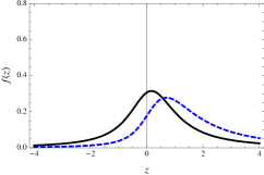
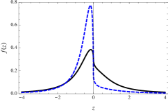
Hence, for $w\sim{\tt Exp}(q)$, the jumps increase the Riccati variable if it is already positive, and decrease it otherwise. Furthermore there is no bound on the magnitude of the jumps. It follows that the effect of increasing the density $p$ of the scatterers is to decrease the density $f$ on ${\mathbb{R}}_{-}$, and to increase it on ${\mathbb{R}}_{+}$. This is in agreement with the plots shown in Figure 7 (a).

For $-w\sim{\tt Exp}(q)$, we observe the opposite effect: as shown in Figure 7 (b), for increasing $p$, the density $f$ is lowered on ${\mathbb{R}}_{+}$ and raised on ${\mathbb{R}}_{-}$. The asymmetry of the plots for a negative strength $w$ is readily explained by using the particle analogy: starting at $+\infty$, the particle rolls down the potential, spurred along by the impurities, and quickly reaches the origin. Once the particle crosses over to the left, the impurities work against the downward force and tend to push the particle back towards the origin.

Figure 7. Plots of the invariant density $f$ for supersymmetric scatterers and positive energy $E=k^{2}=+1$. Black continuous lines correspond to a “low” density of scatterers, i.e. $\theta\sim{\tt Exp}(p)$ with $p=1/2$, and blue dashed lines to a “high” density $p=2$. (a) $w\sim\text{\tt Exp}(1)$. (b) $-w\sim\text{\tt Exp}(1)$.

4.3.2. Product of the form (4.25).

For $E=-k^{2}<0$ and $w\sim{\tt Exp}(q)$, we must take $N=0$ in Equation (4.27) to obtain a normalisable solution. This is consistent with the well-known fact that the spectrum of a supersymmetric Schrödinger Hamiltonian must be contained in $\mathbb{R}_{+}$. Hence

(4.30) $$f(z)=C_{+}^{-1}\frac{z^{-\frac{q}{2}}}{z^{2}-k^{2}}\left(\frac{z-k}{z+k}\right)^{\frac{p}{2k}}\,{\mathbf{1}}_{(k,\infty)}(z)\,.$$

For $-w\sim{\tt Exp}(q)$, the solution is, instead,

(4.31) $$f(z)=C_{-}^{-1}\frac{z^{\frac{q}{2}}}{k^{2}-z^{2}}\left(\frac{k-z}{k+z}\right)^{\frac{p}{2k}}\,{\mathbf{1}}_{(0,k)}(z)\,.$$

By Formula 8 in [23], §3.197,

(4.32) $$C_{\pm}=k^{\mp\frac{q}{2}-1}\,{\tt B}\!\left(\frac{q}{2}+1,\frac{p}{2k}\right)\,{{}_{2}}F_{1}\!\left(\frac{p}{2k}+1,\frac{q}{2}+1;\frac{p}{2k}+\frac{q}{2}+1;-1\right)$$

where ${\tt B}$ is the beta function and ${{}_{2}}F_{1}$ is Gauss’s hypergeometric function.

Figure 8. Plots of the invariant density $f$ for supersymmetric scatterers and negative energy $E=-k^{2}=-1$. Black continuous lines correspond to a “low” density of scatterers, i.e. $\theta\sim{\tt Exp}(p)$ with $p=1/4$, and blue dashed lines to a “high” density $p=4$. (a) $w\sim\text{\tt Exp}(1)$. (b) $-w\sim\text{\tt Exp}(1)$.

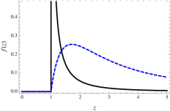
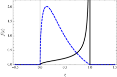
Plots of the invariant density are shown in Figure 8. As before, the particle analogy helps to explain their qualitative features: in view of Equation (4.29), when $w\sim{\tt Exp}(q)$, the “particle” must eventually end up to the right of the equilibrium point $z=k$; see Figure 8 (b). By contrast, when $-w\in{\tt Exp}(q)$ and $z>0$, the Riccati variable remains positive but its value decreases at every jump. Hence, in this case, the support of the invariant density is $(0,k)$; see Figure 8 (b).

4.3.3. Calculation of the characteristic function.

The essential spectrum— and hence also the characteristic function— is invariant under a change of sign of the strength $w$. So we need only consider the case $w\sim{\tt Exp}(q)$. For $E=-k^{2}$, we find, by using Equation (4.30),

$$\mathchoice{{\vbox{\hbox{$\textstyle-$}}\kern-4.86108pt}}{{\vbox{\hbox{$\scriptstyle-$}}\kern-3.25pt}}{{\vbox{\hbox{$\scriptscriptstyle-$}}\kern-2.29166pt}}{{\vbox{\hbox{$\scriptscriptstyle-$}}\kern-1.875pt}}\!\int_{-\infty}^{\infty}\text{d}z\,z\,f(z)=C_{+}^{-1}\int_{k}^{\infty}\text{d}z\,\frac{z^{-\frac{q}{2}+1}}{z^{2}-k^{2}}\left(\frac{z-k}{z+k}\right)^{\frac{p}{2k}}\,.$$

The normalisation constant $C_{+}$ is given explicitly by Formula (4.32), and a similar formula is available for the definite integral; it suffices to replace $q/2$ by $q/2-1$. Using (3.22) and the fact that $N(-k^{2})=0$, the result is

$$\Omega(-k^{2})=-\frac{p}{q}+k\frac{{\tt B}\left(\frac{p}{2k},\frac{q}{2}\right){{}_{2}}F_{1}\left(\frac{p}{2k}+1,\frac{q}{2};\frac{p}{2k}+\frac{q}{2};-1\right)}{{\tt B}\left(\frac{p}{2k},\frac{q}{2}+1\right){{}_{2}}F_{1}\left(\frac{p}{2k}+1,\frac{q}{2}+1;\frac{p}{2k}+\frac{q}{2}+1;-1\right)}\,.$$

This formula extends to other values of the energy by analytic continuation; it suffices to replace $k$ by $\sqrt{-E}$. In particular, for $E=k^{2}>0$, the characteristic function is obtained by replacing $k$ by $-\text{i}k$. The density of states and the Lyapunov exponent may then be deduced from the formulae (see Equation (3.28))

$$N=-\frac{1}{\pi}\,\text{Im}\,\Omega\;\;\text{and}\;\;\gamma=\text{Re}\,\Omega\,.$$

5. Extensions

In this final section, we consider possible extensions of our results: (1) to another scatterer; (2) to another distribution of the strength of the scatterers and (3) to another distribution of the spacing between consecutive scatterers.

5.1. Double impurities

The decomposition formula (1.6) gives a formal correspondence between products of $2\times 2$ matrices and generalised Kronig–Penney models of unit energy where the point scatterers are double impurities. In the particular case

$$\theta\sim{\tt Exp}(p)\,,$$

the density of the invariant measure solves the Frisch–Lloyd equation

(5.1) $$N=(z^{2}+1)f(z)+p\int_{\mathbb{R}}\int_{\mathbb{R}}\text{d}u\,\text{d}w\,\varrho(u,w)\,\int_{z}^{z\text{e}^{-2w}-u}f(y)\,\text{d}y\,.$$

We have already considered the cases where $w$ vanishes almost surely (the delta scatterer) or $u$ vanishes almost surely (the supersymmetric scatterer). The purpose of this subsection is to consider the truly multivariate case where $u$ and $w$ are independent and

$$u\sim{\tt Exp}(q_{d})\,,\;\;w\sim{\tt Exp}(q_{s})\,.$$

We shall show that the corresponding invariant density $f$ solves the differential equation

(5.2) $$\frac{\text{d}}{\text{d}z}\left[2z\left(\varphi^{\prime}-p\,f\right)\right]+\left(q_{s}+2q_{d}z\right)\left(\varphi^{\prime}-p\,f\right)+q_{d}q_{s}\varphi=q_{d}q_{s}N$$

where

$$\varphi:=(z^{2}+1)f(z)$$

and $N$ is independent of $z$. To derive this equation from (5.1), we shall consider the cases $z\leq 0$ and $z>0$ separately.

Consider the latter case; we write

$$\varrho(u,w)=\varrho_{d}(u)\,\varrho_{s}(w)\,.$$

By changing the order of integration, we find

(5.3) $$\int_{0}^{\infty}\text{d}w\,\varrho_{s}(w)\,\int_{z}^{z\text{e}^{-2w}-u}f(y)\,\text{d}y\\ =-\int_{z-u}^{z}f(y)\,\text{d}y+\int_{-u}^{z-u}K_{s}\left(\frac{1}{2}\ln\frac{z}{y+u}\right)f(y)\,\text{d}y\,,$$

where

$$K_{s}(x):=\begin{cases}-\text{e}^{-q_{s}x}&\text{if $x\geq 0$}\\ 0&\text{if $x<0$}\end{cases}\,.$$

So Equation (5.1) becomes

(5.4) $$N=\varphi(z)-p\int_{0}^{\infty}\text{d}u\,\varrho_{d}(u)\int_{z-u}^{z}f(y)\,\text{d}y\\ +p\int_{0}^{\infty}\text{d}u\,\varrho_{d}(u)\int_{-u}^{z-u}K_{s}\left(\frac{1}{2}\ln\frac{z}{y+u}\right)f(y)\,\text{d}y\,,$$

and, by using integration by parts for the first integral on the right-hand side, we find

(5.5) $$N=\varphi(z)-p\int_{0}^{\infty}\text{e}^{-q_{d}u}f(z-u)\,\text{d}u\\ +p\int_{0}^{\infty}\text{d}u\,\varrho_{d}(u)\int_{-u}^{z-u}K_{s}\left(\frac{1}{2}\ln\frac{z}{y+u}\right)f(y)\,\text{d}y\,.$$

Next, differentiate this equation with respect to $z$. By exploiting the identities

$$K_{s}^{\prime}=-q_{s}K_{s}\,,\;\;K_{s}(0+)=1$$

and

$$\frac{\text{d}}{\text{d}u}\text{e}^{-q_{d}u}=-q_{d}\,\text{e}^{-q_{d}u}\,,$$

we deduce

(5.6) $$2z\left[\varphi^{\prime}(z)-p\,f(z)\right]+q_{s}\left[\varphi(z)-N\right]=q_{s}p\int_{0}^{\infty}\text{e}^{-q_{d}u}\,f(z-u)\,\text{d}u\,.$$

The integral term may be eliminated by differentiating once more with respect to $z$, and we obtain eventually Equation (5.2).

The same equation is obtained if, instead, $z<0$. It is a trivial exercise to adapt these arguments to cater for cases where one or both of $u$ and $w$ is always negative. We do not know how to express the solution of this second-order linear differential equation in terms of known functions, except in the limiting cases

$$q_{d}\;\text{fixed}\,,\;q_{s}\rightarrow\infty\,,$$

and

$$q_{d}\rightarrow\infty\,,\;q_{s}\;\text{fixed}\,,$$

that have already been considered in §4.1 and §4.3 respectively.

5.2. Delta scatterers with a gamma distribution

The equation (4.3) with the kernel (4.4) can be reduced to a purely differential form whenever $\varrho$ solves a linear differential equation with piecewise constant coefficients. For instance, suppose that

$$\pm u\sim{\tt Gamma}(2,1/q)\,,$$

i.e.

$$\varrho(u)=\pm q^{2}u\text{e}^{\mp qu}{\mathbf{1}}_{{\mathbb{R}}_{\pm}}(u)\,.$$

Then

$$\left(\frac{\text{d}}{\text{d}u}\pm q\right)^{2}\varrho=0\,.$$

Using the same trick as before, we obtain the following differential equation for $\varphi:=(z^{2}+E)f$:

(5.7) $$\left(\frac{\text{d}}{\text{d}z}\pm q\right)^{2}\varphi-p\left(\frac{\text{d}}{\text{d}z}\pm 2q\right)\frac{\varphi}{z^{2}+E}=q^{2}N\,.$$

Suppose that $E=k^{2}>0$ and use the ansatz

$$\varphi(z):=\exp\left[\mp qz+\frac{p}{k}\arctan\frac{z}{k}\right]h(z)\,.$$

Then

(5.8) $$(z^{2}+k^{2})\,h^{\prime\prime}+p\,h^{\prime}\mp p\,q\,h=0\,.$$

This equation may be solved in terms of hypergeometric series and, by imposing suitable auxiliary conditions, we can find a particular solution $h$ that is positive. The method of variation of constants then yields

(5.9) $$f(z)=\frac{q^{2}N}{z^{2}+k^{2}}\exp\left[\mp qz+\frac{p}{k}\arctan\frac{z}{k}\right]h(z)\\ \times\int_{\mp\infty}^{z}\exp\left[\pm qt-\frac{p}{k}\arctan\frac{t}{k}\right]H(t)\,\text{d}t\,,$$

where

$$H(z):=\frac{\text{e}^{\mp qz}}{h^{2}(z)}\int_{\mp\infty}^{z}\text{e}^{\pm qt}h(t)\,\text{d}t\,.$$

We now return to the calculation of the function $h(z)$ appearing in this formula. The general solution of Equation (5.8) takes a remarkably simple form when

$$p\,q=j(j-1)\,,\;\;j\in{\mathbb{N}}\,.$$

Indeed, substitute

(5.10) $$h(z):=\sum_{i=0}^{\infty}\frac{a_{i}}{i!}z^{i}\,,\;\;a_{0}=1\,,$$

into Equation (5.8). This yields a recurrence relation for the $a_{i}$:

$$k^{2}a_{i+2}=-p\,a_{i+1}+\left[p\,q-i(i-1)\right]a_{i-1}=0\,,\;\;i=0,\,1,\,\ldots\,.$$

By choosing $a_{1}$ so that $a_{j+1}=0$, the infinite series reduces to a polynomial, say $P_{j}$:

$$P_{2}(z)=1+2\,{\frac{pz}{{p}^{2}+2\,{k}^{2}}}+2\,{\frac{{z}^{2}}{{p}^{2}+2\,{k}^{2}}}\,.$$

$$P_{3}(z)=1+6\,{\frac{\left({p}^{2}+4\,{k}^{2}\right)z}{p\left({p}^{2}+10\,{k}^{2}\right)}}+18\,{\frac{{z}^{2}}{{p}^{2}+10\,{k}^{2}}}+24\,{\frac{{z}^{3}}{p\left({p}^{2}+10\,{k}^{2}\right)}}\,.$$

(5.11) $$P_{4}(z)=1+12\,{\frac{p\left({p}^{2}+16\,{k}^{2}\right)z}{{p}^{4}+28\,{p}^{2}{k}^{2}+72\,{k}^{4}}}+72\,{\frac{\left({p}^{2}+6\,{k}^{2}\right){z}^{2}}{{p}^{4}+28\,{p}^{2}{k}^{2}+72\,{k}^{4}}}\\ +240\,{\frac{p{z}^{3}}{{p}^{4}+28\,{p}^{2}{k}^{2}+72\,{k}^{4}}}+360\,{\frac{{z}^{4}}{{p}^{4}+28\,{p}^{2}{k}^{2}+72\,{k}^{4}}}\,.$$

Another solution may be found by setting

$$h(z):=(z^{2}+k^{2})\exp\left[-\frac{p}{k}\arctan\frac{z}{k}\right]\sum_{i=0}^{\infty}\frac{b_{i}}{i!}\,z^{i}\,,\;\;b_{0}=1\,.$$

Then

$$k^{2}b_{i+2}=p\,b_{i+1}+\left[p\,q-(i+2)(i+1)\right]b_{i}=0\,,\;\;i=0,\,1,\,\ldots\,.$$

By choosing $b_{1}$ so that $b_{j-1}=0$, this series reduces to another polynomial, say $Q_{j}$:

$$Q_{2}(z)=1\,.$$

$$Q_{3}(z)=1-\frac{4}{p}z\,.$$

$$Q_{4}(z)=1-10\,{\frac{pz}{6\,{k}^{2}+{p}^{2}}}+30\,{\frac{{z}^{2}}{6\,{k}^{2}+{p}^{2}}}\,.$$

Hence the general solution of Equation (5.8) is

(5.12) $$h(z)=c_{1}P_{j}(z)+c_{2}Q_{j}(z)(z^{2}+k^{2})\exp\left[-\frac{p}{k}\arctan\frac{z}{k}\right]\,.$$

Even with such detailed knowledge, it is not straightforward to identify the particular solution $h$ that yields the density. We end with the remark that the characteristic function may, nevertheless, be constructed by using Halperin’s trick: in this case, the homogeneous version of Equation (3.27) is

$$F^{\prime\prime}(x)+\left\{-E\pm\frac{p/q}{(1\pm\text{i}x/q)^{2}}\left[2\pm\text{i}x/q\right]\right\}F(x)=0\,.$$

The solutions are expressible in terms of Whittaker functions; in particular, for $k$ real,

$$\Omega(k^{2})=\gamma(k^{2})-\text{i}\pi N(k^{2})=2\text{i}k\,\frac{W_{-\text{i}\frac{p}{2k},\frac{\sqrt{1\pm 4pq}}{2}}^{\prime}\left(\mp 2\text{i}kq\right)}{W_{-\text{i}\frac{p}{2k},\frac{\sqrt{1\pm 4pq}}{2}}\left(\mp 2\text{i}kq\right)}\,.$$

This result was originally found by Nieuwenhuizen [35].

5.3. An alternative derivation of the Frisch–Lloyd equation

In deriving Equation (3.14), we made explicit use of the fact that, when the spacing $\theta_{j}:=x_{j+1}-x_{j}$ is exponentially distributed,

$$n(x):=\#\left\{x_{j}:\;x_{j}<x\right\}$$

is a Poisson process. In this subsection, we outline an alternative derivation of the Frisch–Lloyd equation which generalises to other distributions of the $\theta_{j}$.

There is no real loss of generality in setting $E=1$. We use the decomposition

$$A=\begin{pmatrix}\cos\theta&-\sin\theta\\ \sin\theta&\cos\theta\end{pmatrix}\,B\,.$$

Then

$${\mathscr{A}}^{-1}={\mathscr{B}}^{-1}\circ{\mathscr{R}}_{-\theta}$$

where

$${\mathscr{R}}_{\theta}(z):=\frac{z\cos\theta-\sin\theta}{z\sin\theta+\cos\theta}\,.$$

Denote by $\varrho$ the density of the random variable $\theta$ and by $\kappa$ the distribution of $B$. Equation (1.5) for the invariant density $f$ then becomes

(5.13) $$f(z)=\int_{\mathbb{R}}\text{d}\theta\,\varrho(\theta)\int_{\text{SL}\left(2,{\mathbb{R}}\right)}\kappa(\text{d}B)\left[f\circ{\mathscr{B}}^{-1}\circ{\mathscr{R}}_{-\theta}\right](z)\frac{\text{d}}{\text{d}z}\left[{\mathscr{B}}^{-1}\circ{\mathscr{R}}_{-\theta}\right](z)\\ =\int_{\mathbb{R}}\text{d}\theta\,\varrho(\theta)\int_{\text{SL}\left(2,{\mathbb{R}}\right)}\kappa(\text{d}B)\left[f\circ{\mathscr{B}}^{-1}\right](w)\frac{\text{d}{\mathscr{B}}^{-1}}{\text{d}z}(w)\,\frac{\partial w}{\partial z}$$

where

$$w:={\mathscr{R}}_{-\theta}(z)=\frac{z\cos\theta+\sin\theta}{-z\sin\theta+\cos\theta}\,.$$

The same equation can also be written in the more compact form

(5.14) $$f(z)=\int_{\mathbb{R}}\text{d}\theta\,\varrho(\theta)\frac{\partial}{\partial z}\int_{\text{SL}\left(2,{\mathbb{R}}\right)}\kappa(\text{d}B)\int_{0}^{{\mathscr{B}}^{-1}(w)}\text{d}tf(t)\,.$$

Now,

$$\frac{\partial w}{\partial\theta}=(1+z^{2})\frac{\partial w}{\partial z}\,.$$

Hence, if we multliply Equation (5.14) by $1+z^{2}$, we obtain

$$(1+z^{2})f(z)=\int_{\mathbb{R}}\text{d}\theta\,\varrho(\theta)\frac{\partial}{\partial\theta}\int_{\text{SL}\left(2,{\mathbb{R}}\right)}\kappa(\text{d}B)\int_{0}^{{\mathscr{B}}^{-1}(w)}\text{d}tf(t)\,.$$

Next, differentiate with respect to $z$:

(5.15) $$\frac{\text{d}}{\text{d}z}\left[(1+z^{2})f(z)\right]=\int_{\mathbb{R}}\text{d}\theta\,\varrho(\theta)\frac{\partial^{2}}{\partial z\partial\theta}\int_{\text{SL}\left(2,{\mathbb{R}}\right)}\kappa(\text{d}B)\int_{0}^{{\mathscr{B}}^{-1}(w)}\text{d}tf(t)\\ =\int_{\mathbb{R}}\text{d}\theta\,\varrho(\theta)\frac{\partial^{2}}{\partial\theta\partial z}\int_{\text{SL}\left(2,{\mathbb{R}}\right)}\kappa(\text{d}B)\int_{0}^{{\mathscr{B}}^{-1}(w)}\text{d}tf(t)\,.$$

We may then use integration by parts for the outer integral; in the particular case

$$\varrho(\theta)=p\text{e}^{-p\theta}{\mathbf{1}}_{[0,\infty)}$$

the Frisch–Lloyd equation (3.14) follows easily after invoking (5.14) once more.

We can use the same trick whenever the density of $\theta$ satisfies a linear differential equation with constant coefficients. For instance, in the case

$$\theta\sim{\tt Gamma}(2,p)$$

it may be shown that

$$\frac{\text{d}}{\text{d}z}\left[(1+z^{2})\varphi^{\prime}(z)\right]-2p\varphi^{\prime}(z)+p^{2}f(z)=p^{2}\int_{\text{SL}\left(2,\mathbb{R}\right)}\kappa(\text{d}B)\left[f\circ{\mathscr{B}}^{-1}\right](z)\frac{\text{d}{\mathscr{B}}^{-1}}{\text{d}z}(z)$$

where

$$\varphi(z)=(1+z^{2})f(z)\,.$$

6. Conclusion

In this article we have studied the invariant measure of products of random matrices in $\text{SL}\left(2,{\mathbb{R}}\right)$. This study relied on the correspondence between such products and a certain class of random Schrödinger equations in which the potential consists of point scatterers. We have considered several instances of this correspondence: delta, delta-prime and supersymmetric scatterers. By generalising the approach developed by Frisch & Lloyd for delta scatterers, we have obtained an integral equation for the invariant density of a Riccati variable; this density yields the invariant measure of the product of random matrices. For the three cases of point scatterers we have obtained explicit formulae for the invariant measures. These are the main new results of this paper.

The integrated density of states and the Lyapunov exponent of these models were also calculated. Two approaches were used for this purpose: the first is “Halperin’s trick” and is specific to the case of delta scatterers (cf. section 3.5); the second uses analytic continuation of the characteristic function and depends on the explicit knowledge of the invariant measure in some interval of the energy outside the spectrum. By the first of these methods we have recovered the results of Nieuwenhuizen in the case of delta scatterers. By the second method we have found new explicit formulae for the integrated density of states and for the Lyapunov exponent in the cases of delta-prime and of supersymmetric scatterers.

All these analytical results were obtained when the spacing between consecutive scatterers, as well as the impurity strength, have exponential distributions. Possible extensions to the gamma distribution were also discussed.

A more complicated type of scatterer, combining the delta and the supersymmetric scatterers, has also been examined. We called this scatterer the “double impurity”; it is interesting because every product of matrices in $\text{SL}\left(2,{\mathbb{R}}\right)$ may in principle be studied by considering a Schrödinger problem whose potential consists of double impurities. Although we succeeded in deriving a differential equation for the invariant measure associated with a particular distribution of such scatterers, we were unable to express its solution in terms of known functions.

In this paper we have played down the physical aspects of the models. Apart from the inverse localisation length and the density of states, there are other physical quantities that bear some relation to the Riccati variable and whose statistical properties are of interest. Let us mention three of them: the most obvious is the phase of the reflexion coefficient on the disordered region; for a semi-infinite disordered region, its distribution is trivially related to the invariant density of the Riccati variable [5, 22, 32]. Another quantity is the Wigner time delay (the derivative of the phase shift with respect to the energy); it has been considered in the contexts of the Schrödinger [28, 40] and Dirac [39] equations. A third quantity is the transmission coefficient (i.e. conductance) [4, 16, 37]. The study of the distributions of the Wigner time delay and of the transmission coefficient is mathematically more challenging because it requires the analysis of some joint distributions; for this reason it has been confined so far to limiting cases.

Some of the physical aspects arising from our results will form the basis of future work.

Appendix A Scattering, transfer and boundary matrices

We discuss in this section the relationship between the scattering matrix $S$, defined by (2.9), and the boundary matrix $B$, defined by (2.3). Here we need not assume that the scatterer is necessarily pointlike; the scattering matrix and the corresponding boundary matrix could equally well describe the effect of a potential supported on an interval.

We first write the scattering matrix in terms of transmission and reflexion probability amplitudes $t$, $t^{\prime}$ and $r$, $r^{\prime}$ :

$$S=\begin{pmatrix}r&t^{\prime}\\ t&r^{\prime}\end{pmatrix}\>.$$

Current conservation implies

$$|a^{\text{out}}_{+}|^{2}+|a^{\text{out}}_{-}|^{2}=|a^{\text{in}}_{-}|^{2}+|a^{\text{in}}_{+}|^{2}$$

and so forces the scattering matrix to be unitary, i.e. $S\in U(2)$. The constraints on the coefficients, namely

$$|r|^{2}+|t|^{2}=|r^{\prime}|^{2}+|t^{\prime}|^{2}=|r^{\prime}|^{2}+|t|^{2}=|r|^{2}+|t^{\prime}|^{2}=1\,,$$

$${r^{\prime}}/{t^{\prime}}=-\overline{{r}/{t}}\;\;\text{and}\;\;{r}/{t^{\prime}}=-\overline{{r^{\prime}}/{t}}\,,$$

are conveniently built into the following parametrisation, which also illustrates the factorisation $U(2)=U(1)\times{}SU(2)$:

(A.1) $$S=\text{i}\text{e}^{\text{i}\theta}\begin{pmatrix}\text{e}^{\text{i}\varphi}\sqrt{1-\tau}&-\text{i}\text{e}^{-\text{i}\chi}\sqrt{\tau}\\[2.84544pt] -\text{i}\text{e}^{\text{i}\chi}\sqrt{\tau}&\text{e}^{-\text{i}\varphi}\sqrt{1-\tau}\end{pmatrix}\>.$$

This representation of the scattering matrix is interesting because the four real parameters have a clear physical interpretation: $\tau\in[0,1]$ is the probability of transmission through the scatterer; $\theta$ is the global phase of the matrix, i.e.

$$\det{}S=-\text{e}^{2\text{i}\theta}\,.$$

It is sometimes referred to as the “Friedel phase” since it is the phase appearing in the Krein–Friedel sum rule relating the local density of states of the scattering region to a scattering property. The phase $\varphi$ is a measure of the left-right asymmetry ($\varphi=0$ or $\pi$ corresponds to a scattering invariant under $x\to-x$). Finally the phase $\chi$ is of magnetic origin, since time reversal corresponds to transposition of the scattering matrix.

Next, we introduce the transfer matrix $T$ relating left and right amplitudes:

$$\begin{pmatrix}a^{\text{out}}_{+}\\[2.84544pt] a^{\text{in}}_{+}\end{pmatrix}=T\begin{pmatrix}a^{\text{in}}_{-}\\[2.84544pt] a^{\text{out}}_{-}\end{pmatrix}\hskip 14.22636pt\mbox{where}\hskip 14.22636ptT=\begin{pmatrix}\overline{1/t}&-\overline{r/t}\\[2.84544pt] -r/t^{\prime}&1/t^{\prime}\end{pmatrix}\>.$$

This matrix is useful when considering the cumulative effect of many scatterers because it follows a simple composition law. Again, current conservation implies that the transfer matrix is unitary:

$$\left|a_{+}^{\text{out}}\right|^{2}-\left|a_{+}^{\text{in}}\right|^{2}=\left|a_{-}^{\text{in}}\right|^{2}-\left|a_{-}^{\text{out}}\right|^{2}\,.$$

In other words, $T\in{}U(1,1)$ (note that $\det{}T=t/t^{\prime}=\text{e}^{2\text{i}\chi}$).

The boundary matrix is also a “transfer matrix” in the sense that it connects properties of the wavefunction on both sides of the scatterer. The relation between $T$ and $B$ is easily found: from

$$\begin{pmatrix}\psi^{\prime}(0\pm)\\ \psi(0\pm)\end{pmatrix}=\begin{pmatrix}\text{i}k&-\text{i}k\\ 1&1\end{pmatrix}\begin{pmatrix}a_{\pm}^{\begin{subarray}{c}\text{out}\\ \text{in}\end{subarray}}\\[2.84544pt] a_{\pm}^{\begin{subarray}{c}\text{in}\\ \text{out}\end{subarray}}\end{pmatrix}$$

we deduce

$$B=U\,T\,U^{\dagger}\hskip 14.22636pt\mbox{where}\hskip 14.22636ptU=\frac{\text{e}^{-\text{i}\pi/4}}{\sqrt{2k}}\begin{pmatrix}\text{i}k&-\text{i}k\\ 1&1\end{pmatrix}\>.$$

Then, using the parametrisation (A.1), we arrive at the following alternative form of Equation (2.3):

(A.2) $$B=\frac{\text{e}^{\text{i}\chi}}{\sqrt{\tau}}\begin{pmatrix}\cos\theta-\sin\varphi\,\sqrt{1-\tau}&-k\left[\sin\theta+\cos\varphi\,\sqrt{1-\tau}\right]\\[2.84544pt] \frac{1}{k}\left[\sin\theta-\cos\varphi\,\sqrt{1-\tau}\right]&\cos\theta+\sin\varphi\,\sqrt{1-\tau}\end{pmatrix}$$

In particular, this expression shows clearly that

$$\text{e}^{-\text{i}\chi}B\in\mathrm{SL}(2,{\mathbb{R}})\,.$$

In one dimension, if a magnetic field is present, it may always be removed by a gauge transformation. Furthermore, setting the magnetic phase in the exponential factor to zero does not affect the spectrum of the Schrödinger operator. Hence there is no loss of generality in restricting our attention to the case $B\in\mathrm{SL}(2,{\mathbb{R}})$.

We end this appendix with some examples of scatterers, expressed in terms of the parameters $\chi$, $\tau$, $\theta$ and $\varphi$.

Example 1.

For $\tau=1$, $\varphi=0$ and $\chi=0$, $B$ is the matrix describing a rotation of angle $\theta=k\ell$. In this case, the “scattering” is equivalent to free propagation through an interval of length $\ell$.

Example 2.

The scattering matrix for the delta impurity may be written as

$$S=\text{e}^{\text{i}\theta}\begin{pmatrix}\text{i}\sin\theta&\cos\theta\\ \cos\theta&\text{i}\sin\theta\end{pmatrix}$$

where

$$\theta=-\arctan\frac{u}{2k}\in(-\pi/2,\,\pi/2)\,.$$

The other parameters are given by $\chi=0$,

$$\varphi=\begin{cases}0&\text{if $u<0$}\\ \pi&\text{if $u>0$}\end{cases}$$

and

$$\tau=\left[1+\left(\frac{u}{2k}\right)^{2}\right]^{-1}\,.$$

Example 3.

For the delta-prime scatterer, the scattering matrix $S$ has the same form as in the previous example, but this time with

$$\theta=\arctan\frac{vk}{2}\in(-\pi/2,\,\pi/2)\,,$$

$$\chi=0\,,$$

$$\varphi=\begin{cases}0&\text{if $v<0$}\\ \pi&\text{if $v>0$}\end{cases}\,,$$

and

$$\tau=\left[1+\left(\frac{vk}{2}\right)^{2}\right]^{-1}\,.$$

Example 4.

The supersymmetric scatterer corresponds to taking $\chi=\theta=0$, $\varphi=-\pi/2$ and $\tau=\text{sech}^{2}w$.

References

- [1] M. Abramowitz and I. A. Stegun, Handbook of Mathematical Functions, Dover, New York, 1965.
- [2] S. Albeverio, L. Dabrowski and P. Kurasov, Symmetries of the Schrödinger operators with point interactions, Lett. Math. Phys. 45 (1998) 33–47.
- [3] S. Albeverio, F. Gesztesy, R. Høegh-Krohn and H. Holden, Solvable Models in Quantum Mechanics, Springer–Verlag, Berlin, 1988.
- [4] T. N. Antsygina, L. A. Pastur and V. A. Slyusarev, Localization of states and kinetic properties of one-dimensional disordered systems, Sov. J. Low Temp. Phys. 7 (1981) 1–21.
- [5] C. Barnes and J.-M. Luck, The distribution of the reflection phase of disordered conductors, J. Phys.A: Math. Gen. 23 (1990) 1717.
- [6] P. Bougerol and J. Lacroix, Products of Random Matrices with Applications to Schrödinger Operators, Birhaüser, Basel, 1985.
- [7] J.-P. Bouchaud, A. Comtet, A. Georges, and P. Le Doussal, Classical diffusion of a particle in a one-dimensional random force field, Ann. Phys. (N.Y.) 201 (1990) 285–341.
- [8] P. Carmona, F. Petit and M. Yor, On the distribution and asymptotic results for exponential functionals of Lévy processes, in: M. Yor (editor), Exponential Functionals and Principal Values Related to Brownian Motion, pp. 173-221, Biblioteca de la Revista Matemática Iberoamericana, con la colaboración de la Universidad autónoma de Madrid, 1997.
- [9] R. Carmona and J. Lacroix, Spectral Theory of Random Schrödinger Operators, Birkhaüser, Boston, 1990.
- [10] J.–F. Chamayou and G. Letac, Explicit stationary distributions for compositions of random functions and products of random matrices, J. Theor. Prob. 4 (1991) 3–36.
- [11] T. Cheon and T. Shigehara, Continuous spectra of generalized Kronig-Penney model, J. Phys. Soc. Jpn. 73 (2004) 2986–2990.
- [12] T. Cheon and T. Shigehara, Realizing discontinuous wave functions with renormalized short-range potentials, Phys. Lett. A 243 (1998) 111–116.
- [13] P. R. Chernoff and R. J. Hughes, A new class of point interactions in one dimension, J. Funct. Anal. 111 (1993) 97–117.
- [14] A. Comtet and C. Texier, One-dimensional disordered supersymmetric quantum mechanics: a brief survey, in Supersymmetry and Integrable Models, edited by H. Aratyn et al, Lecture Notes in Physics, Vol. 502, pages 313–328, Springer, 1998, (also available as cond-mat/97 07 313).
- [15] F. Cooper, A. Khare and U. P. Sukhatme, Supersymmetry in Quantum Mechanics, World Scientific, Singapore, 2001.
- [16] L. I. Deych, A. A. Lisyansky and B. L. Altshuler, Single parameter scaling in 1-D Anderson localization. Exact analytical solution, Phys. Rev. B 64 (2001) 224202.
- [17] P. Exner, Lattice Kronig-Penney models, Phys. Rev. Lett. 74 (1995) 3503.
- [18] W. Feller, An Introduction to Probability Theory and its Applications, vol. 2, Wiley, New York, 1971.
- [19] H. L. Frisch and S. P. Lloyd, Electron levels in a one-dimensional lattice, Phys. Rev. 120 (1960) 1175–1189.
- [20] H. Furstenberg, Noncommuting random products, Trans. Amer. Math. Soc. 108 (1963) 377–428.
- [21] H. K. Gjessing and J. Paulsen, Present value distributions with application to ruin theory and stochastic equations, Stochastic Process. Appl. 71 (1997) 123–144.
- [22] I. Goldhirsch, S. H. Noskowicz and Z. Schuss, Spectral degeneracy in the one-dimensional Anderson problem: A uniform expansion in the energy band, Phys. Rev. B 49 (1994) 14504–14522.
- [23] I. S. Gradstein and I. M. Ryzhik In: A. Jeffrey, Editor, Tables of Integrals, Series and Products, Academic Press, New York, 1964.
- [24] V. Gurarie and J. T. Chalker, Bosonic excitations in random media, Phys. Rev. B 68 (2003) 134207.
- [25] B. I. Halperin, Green’s functions for a particle in a one-dimensional random potential, Phys. Rev. 139 (1965) A104–A117.
- [26] D. C. Herbert and R. Jones, Localized states in disordered systems, J. Phys. C: Solid State Phys. 4 (1971) 1145.
- [27] K. Ishii, Localization of eigenstates and transport phenomena in the one dimensional disordered system, Prog. Theor. Phys. (Suppl.) 53 (1973) 77–138.
- [28] A. M. Jayannavar, G. V. Vijayagovindan and N. Kumar, Energy dispersive backscattering of electrons from surface resonances of a disordered medium and noise, Z. Phys. B – Condens. Matter 75 (1989) 77.
- [29] S. Kotani, On asymptotic behaviour of the spectra of a one-dimensional Hamiltonian with a certain random coefficient, Publ. RIMS, Kyoto Univ. 12 (1976) 447–492.
- [30] R. de L. Kronig and W. G. Penney, Quantum mechanics of electrons in crystal lattices, Proc. Roy. Soc. London A 130 (1931) 499–513.
- [31] I. M. Lifshits, S. A. Gredeskul and L. A. Pastur, Introduction to the Theory of Disordered Systems, Wiley, New York, 1988.
- [32] J.-M. Luck, Systèmes désordonnés unidimensionnels, Alea, Saclay, 1992.
- [33] J. Marklof, Y. Tourigny and L. Wolowski, Explicit invariant measures for products of random matrices, Trans. Amer. Math. Soc. 360 (2008) 3391–3427.
- [34] T. M. Nieuwenhuizen, A new approach to the problem of disordered harmonic chains, Physica A 113 (1982) 173–202.
- [35] T. M. Nieuwenhuizen, Exact electronic spectra and inverse localization lengths in one-dimensional random systems: I. Random alloy, liquid metal and liquid alloy, Physica A 120 (1983) 468–514.
- [36] M. Pollicott, Maximal Lyapunov exponents for random matrix products, Invent. Math. (2010) DOI: 10.1007/S00222-004-0357-4.
- [37] H. Schomerus and M. Titov, Band-center anomaly of the conductance distribution in one-dimensional Anderson localization, Phys. Rev. B 67 (2003) 100201.
- [38] P. S̆eba, The generalized point interaction in one dimension, Czech. J. Phys. 36 (1986) 667–673.
- [39] M. Steiner, Y. Chen, M. Fabrizio and A. O. Gogolin, Statistical properties of localization-delocalization transition in one dimension, Phys. Rev. B 59 (1999) 14848.
- [40] C. Texier and A. Comtet, Universality of the Wigner time delay distribution for one-dimensional random potentials, Phys. Rev. Lett. 82 (1999) 4220–4223.
- [41] C. Texier and C. Hagendorf, One-dimensional classical diffusion in a random force field with weakly concentrated absorbers, Europhys. Lett. 86 (2009) 37011.
- [42] D. J. Thouless, A relation between the density of states and range of localization for one-dimensional random systems, J. Phys. C: Solid State Phys. 5 (1972) 77.