Luminous Red Galaxies in Simulations: Cosmic Chronometers?
Abstract
There have been a number of attempts to measure the expansion rate of the universe at high redshift using Luminous Red Galaxies (LRGs) as ”chronometers”. The method generally assumes that stars in LRGs are all formed at the same time. In this paper, we quantify the uncertainties on the measurement of H(z) which arise when one considers more realistic, extended star formation histories. In selecting galaxies from the Millennium Simulation for this study, we show that using rest-frame criteria significantly improves the homogeneity of the sample and that can be recovered to within 3% at even when extended star formation histories are considered. We demonstrate explicitly that using Single Stellar Populations to age-date galaxies from the semi-analytical simulations provides insufficient accuracy for this experiment but accurate ages are obtainable if the complex star formation histories extracted from the simulation are used. We note, however, that problems with SSP-fitting might be overestimated since the semi-analytical models tend to over predict the late-time star-formation in LRGs. Finally, we optimize an observational program to carry out this experiment.
keywords:
galaxies - galaxies: evolution - cosmological parameters - cosmology: observations1 Introduction
An important constraint on cosmological models is the evolution of the Hubble parameter, which is defined as:
| (1) |
Most tests of cosmology use measures of the luminosity distance or the angular diameter distance, which include an integral over , but measuring directly can potentially provide a more direct constraint on cosmological parameters (Jimenez & Loeb 2002). can be determined at high redshifts by measuring the time-interval, , corresponding to a redshift interval, , to obtain an approximation of the derivative in equation (1). A number of authors have attempted to use this method (Ferreras, Mechiorre, & Silk 2001, Jimenez & Loeb 2002, Jimenez et al. 2003, Capozziello et al. 2004, Ferreras, Melchoirre, & Tocchini-Valentini 2003, Simon et al. 2005, Dantas et al. 2007, Verkhodanov, Parijskij, & Starobinsky 2007, Samushia et al. 2009) to track the evolution of as a function of redshift, and place constraints on cosmological parameters. Most recently, Stern et al. (2010) extended the studies of Jimenez et al. (2003) to a larger, more homogeneous sample to make the measurement of H(z) from LRGs.
Jimenez & Loeb (2002) suggested using spectroscopic age-dating of Luminous Red Galaxies (LRGs) to measure . LRGs are galaxies selected from the Sloan Digital Sky Survey (SDSS, York et al. 2000) by apparent magnitude to trace the evolution of a homogeneous, volume-limited sample of red galaxies (Eisenstein et al. 2001). Jimenez et al. (2003) used LRGs from the SDSS to measure km s-1 Mpc-1 (the Hubble parameter at z=0). Simon et al. (2005) used the same method to find as a function of redshift for . In both cases, the authors assume that LRGs are drawn from the same parent population with the bulk of their stars formed at high redshift and fit single-burst equivalent ages to the galaxies. Although there is evidence that LRGs make up a fairly homogeneous population of galaxies consisting mostly of old populations, Roseboom et al. (2006) have shown that this is not completely true. Furthermore, Barber et al. (2007) find that these galaxies have a range of formation ages and stellar histories. Jimenez and Loeb (2002) note that galaxies would not have formed at exactly the same time and explore what effect this would have on one’s ability to discriminate between different models for w(z). They do not, however, discuss the consequences of star formation being extended over a period in each galaxy (they assume all stars form at exactly the same time in a galaxy). This extended star formation history (SFH) needs to be considered when one defines and measures an age for a galaxy. In Jimenez et al (2003), the question is addressed in a little more detail: they simulate LRG spectra and add a contribution from a small fraction of stars formed at late times; they then age-date the galaxies and conclude that the age ”edge” is not significantly different from the theoretical expectation. They do not attempt to quantify what uncertainties arise as a result of the extended star formation.
Given the importance of correct estimates of uncertainties on the measured H(z), we explore, in this paper, the uncertainties that arise from LRGs having extended and varied SFHs. We use LRGs identified in the Millennium Simulation (MS, Springel et al. 2005) since the only way to reliably determine uncertainties is in a simulation where the SFH and input cosmology are known. The MS is currently one of the most detailed simulations of the evolution of galaxies and large-scale structure and has been tuned to reflect observational data. Almeida et al. (2008) studied LRGs in simulations and showed that the luminosity function and the clustering of LRGs are reasonably well-modelled in their semi-analytical models of galaxy evolution, which also reproduce many other observables. The parameters of the de Lucia et al. (2006) semi-analytical model have also been successfully tuned to match the luminosity, colour, and morphology of local elliptical galaxies, the more massive candidates of which would be LRGs.
On the other hand, galaxies are not modelled perfectly in the simulations: there are indications that model galaxies assemble later than observations may suggest (Collins et al. 2009) but more reliable estimates of stellar mass are required. It should be noted that these models overestimate the small amount of evolution seen in the properties of LRGs (Wake et al. 2006, 2008) and likely over predict the amount of growth occurring in these sources (Masjedi et al. 2008). Specifically for LRGs, Barber et al. (2007) find similar star formation rates, but younger ages than the de Lucia models. In addition, properties of local galaxies can be reproduced with different models for galaxy formation (e.g. Kereš et al. 2009). However, the simulations provide viable models of extended SFHs, allowing us to quantify associated uncertainties and optimize analysis methods before applying them to observational data.
In this paper, we optimize the selection of LRGs based on their properties in the MS and examine how well can be recovered from their mass-weighted age. To explore and quantify the uncertainties associated with extended SFHs, we then investigate how well can be determined, if the mass-weighted age of these LRGs were measurable, using three different methods. In practice, mass-weighted ages are not directly measurable and accurate age-dating using LRG spectra is potentially a bigger challenge for the cosmic chronometer approach. We carry out an initial study of age-dating, and its implications for measurements, using the stellar population models of Bruzual & Charlot (BC2003, 2003) to synthesize spectra. In contrast to fitting only single stellar population models (SSPs) (e.g. Simon et al. 2005) or dual-burst population models (Jimenez et al. (2003)) to determine the LRG spectral ages, we make a comparison of SSP results to those using more complicated SFHs. In a companion paper (Olivier et al. 2009), we delve much deeper into issues of age-dating galaxy spectra.
The outline of the paper is as follows: In §2 we discuss the extraction of LRGs from the MS. In §3 we investigate how well is recovered in the MS using LRGs identified in the simulation. In §4, we describe the modelling and age-dating of LRG spectra. In §5, we discuss an observational program to measure . We summarize our results and conclusions in §6. Throughout this work, we adopt the cosmology used in de Lucia et al. (2006) of , , and .
2 Identifying LRGs in the Millennium Simulation
The Millennium Simulation is a dark-matter-only N-body simulation run using the Gadget code of Springel et al. (2005). The simulation has particles distributed in a 500 Mpc3 box. Dark matter halos are identified in snapshots of the simulation at 63 different times and merger trees of halos are constructed. Semi-analytical modelling of galaxy evolution is carried out using the merger trees, providing a catalogue of galaxies in each snapshot, where each galaxy has an array of observational properties associated with it (Baugh et al. 2005, Bower et al. 2006, de Lucia et al. 2006). Properties of the halos and simulated galaxies are stored in a database which can be accessed from the web.
Here, we focus on the galaxy catalogues constructed using the semi-analytical models of de Lucia et al. (2006). We identify simulated galaxies with LRG properties in various snapshots (corresponding to a particular set of redshifts near ) and then extract the star formation histories. The model does reproduce many properties of local galaxies and LRGs (Croton et al. 2006, de Lucia et al. 2006), but a number of weakness are apparent as outlined in the introduction.
In addition to the de Lucia models, we examined the models by Bower et al. (2006, hereafter Durham models), which also uses the Millennium Simulation. However, the two models are different in the implementation of their semi-analytical models. For our purposes, the most relevant difference between the models is in their handling of gas cooling, star formation, and feedback as these are directly related to the star formation histories of the galaxies. We save the comparison of other semi-analytical models and how they would affect the calculation of for future work.
2.1 Selecting LRGs using SDSS criteria
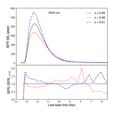
Initially we extracted LRGs using the apparent magnitude constraints for SDSS data from Eisenstein et al. (2001). Our target redshift is close to the redshift where the SDSS ‘Cut I’ must be replaced with the ‘Cut II’ colour selection criteria (At , the Balmer break moves into the r-band and a different colour selection is required to identify LRGs). In Fig. 1, we plot the average SFH for three redshift snapshots at . The SFHs, especially once normalized to the SFH at , show significant differences. Importantly, there is no monotonic behaviour for successive . In Table 1, we summarize the average formation parameters for the population. There is a significant dispersion in formation redshift (), the redshift of peak star formation (), and the redshift of last major star formation epoch (), which is defined as the redshift where the star formation rate falls below 10 . For galaxies in the MS at , almost have had a burst of star formation greater than 5 in the previous gigayear and up to are greater than 3 away from the average star formation history.
In addition, the change in the average mass-weighted age, , does not correspond to the change in the age of the Universe at these redshifts. Between , the age of the simulated Universe changes by 1.13 Gyr, whereas the change in corresponds to 1.27 Gyr. For , the values are 0.26 and 0.18 Gyr, respectively. A key assumption of this technique is that the galaxies are passively evolving. If true, then the change in their age with redshift should corresponding to the change in the age of the Universe. However, that is not the case for this sample.
The sample selected using the SDSS cuts in the MS are not very homogeneous. A source of this inhomogeneity is the selection of galaxies in apparent magnitude space. Due to the width of the redshift bin within which the apparent colour cuts are defined, different types of galaxies are selected near the edges of the redshift bin including a large number of galaxies that have more extended SFHs. Inclusion of these galaxies decreases the sensitivity of this method for determining . Furthermore, the observing efficiency is reduced if only the oldest galaxies are used unless they can be pre-selected.
| Cut | z | 111The fraction of galaxies with within 1 Gyr of the redshift. | |||||
|---|---|---|---|---|---|---|---|
| SDSS | 0.32 | 0.32 | 0.13 | ||||
| SDSS | 0.46 | 0.03 | 0.19 | ||||
| SDSS | 0.51 | 0.29 | 0.17 | ||||
| Our Cut | 0.32 | 0.14 | 0.15 | ||||
| Our Cut | 0.46 | 0.14 | 0.15 | ||||
| Our Cut | 0.51 | 0.14 | 0.15 |
2.2 Selecting a more homogeneous sample
Since the age-dating experiment assumes a similar SFH for LRGs at different redshifts, we explored other selection criteria that would yield a more homogeneous set of objects. The MS includes rest-frame luminosities, and instead of the SDSS selection, we chose to use absolute magnitude cuts in the rest-frame to select LRG-like objects. In a real age-dating experiment, this would require having a large sample of galaxies with multi-band photometry and spectroscopic (or high quality photometric) redshifts. For , this selection can easily be done from the SDSS data (e.g. the 2SLAQ catalog of Cannon et al. 2006).
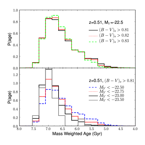
The effect of varying the colour and brightness on the normalized distribution of mass-weighted ages of simulated galaxies is shown in Fig. 2 for galaxies at . We demonstrate that by selecting the brightest galaxies, we are able to select galaxies with narrower SFHs; that is, galaxies in which more of the stars are formed at earlier times. In the lower panel, we show the effect of changing the colour-cut, demonstrating that the SFHs are not very sensitive to the rest-frame colour-cut we choose. Using these results, we decided to use a rest-frame colour-cut of and an absolute magnitude cut of . A brighter magnitude cut does produce an even more homogeneous sample, but results in a dramatic drop in the number of sources (a factor of 10 decrease with a 0.5 mag increase).
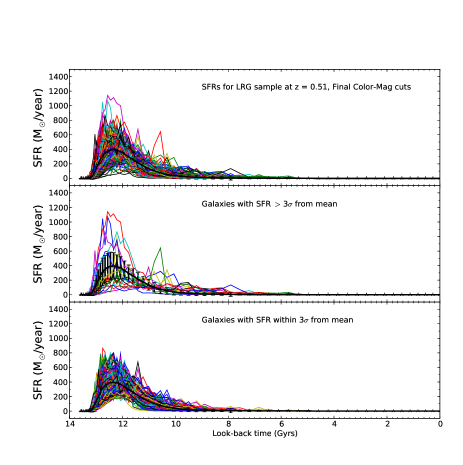
In Fig. 3, we plot the average SFHs of galaxies selected using our rest-frame cuts at four redshifts (upper panel) as well as the ratio of SFR to that obtained at z=0.32 (lower panel). It is clear, as compared to Fig. 1, that the galaxies selected in this way have more homogeneous SFHs, and the small change from low to high redshift is monotonic. To demonstrate the variation in SFH for galaxies selected in this way at a particular redshift, we plot, in Fig. 4, SFHs of 200 randomly chosen galaxies from the sample at . In the lower panels, we break the 100 galaxies into two samples: those that are more than 3 away from the mean and those that are within 3 of the mean.
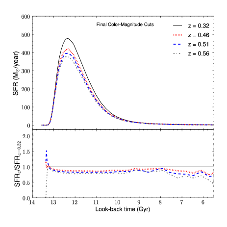
The formation properties of these galaxies are compared to the SDSS sample in Table 1. On average, this population shows similar dispersion to the objects selected from the SDSS cuts. However, a smooth and gradual change is evident for our cut as opposed to the dramatic change seen using the SDSS cuts. In addition, a constant and lower percentage of objects have had significant events of star formation in the past as opposed to the SDSS cuts.
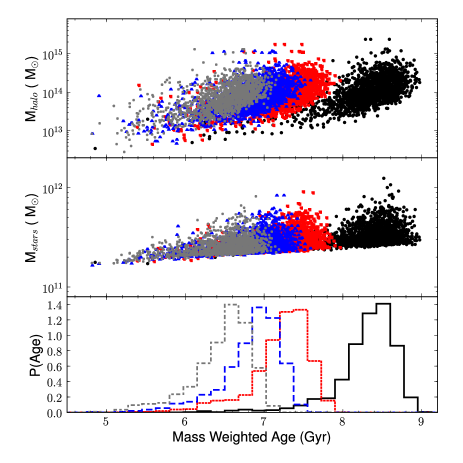
To investigate further the properties of the LRGs selected with the new cuts, we plot, in the top panel of Fig. 5, the mass of the halo which hosts the galaxies vs. the mass-weighted age of our selected LRGs for four snapshots. We note the more massive halos contain older galaxies, a correlation which arises naturally in hierarchical structure formation scenarios (de Lucia et al. 2006) and corresponds to the observed phenomenon of downsizing (Cowie et al. 1996).
In addition, these galaxies have large stellar masses with values typically above with a peak value just above . There is a strong, lower mass cut-off in each of the redshift bins due to the absolute magnitude cut in the selection function. The overall stellar mass values are in good agreement for stellar masses calculated for LRGs by Barber et al. (2007), but their data does not show the strong correlation between age and stellar mass for SDSS selected LRGs that is seen in the de Lucia models.
When we substitute metallicity for halo mass, we see no correlation. The lower panel of Fig. 5 shows a normalized distribution of the mass-weighted ages of galaxies from our selection. Even at very close redshifts, the ages of the galaxies are separated into distinct groups, although a small tail of younger galaxies is still present.
For the rest of the paper, we refer to these galaxies as LRGs. Galaxies selected using the old cut will be referred to as SDSS LRGs. At four different redshift (), the total number of LRGs extracted from the MS are 1705, 1491, 1448, and 1337 galaxies respectively.
2.3 Selecting LRGs from Durham Models
We applied both the SDSS and the absolute magnitude cuts to the Durham model. Although similar density of objects were found in the Durham model at z=0.51 by using the SDSS cuts, the density of LRGs after the absolute magnitude cut was down by an order of magnitude as compared to both the real object density and the de Lucia model. This was due to the lack of bright objects in the Durham model at intermediate redshifts. This was previously shown by Almeida et al. (2008) in the mismatch between the observed luminosity function of 2SLAQ LRGs and the Durham models, where the Durham model has an excess of faint LRGs.
For the selection of objects that were found in the Durham model, they had an elevated level of star formation, bluer colors, less regular stellar histories, and a large spread in the stellar ages. These results are consistent with results found by Almeida et al. (2008) and Gonzalez et al. (2009) in studies of the Durham model and LRGs. Further study is necessary to ascertain the reasons for the differences between the models and the observations, and for this reason, we focus on the results from the de Lucia models for the remainder of this paper.
3 Recovering from Millennium LRGs
In this section, we explore the uncertainties on related to the extended star formation histories of LRGs and ignore difficulties associated with measuring the age of LRGs. We use only the galaxies selected with our rest-frame magnitude and color cuts. We use the mass-weighted ages, which are shown in the bottom panel of Fig. 5, for galaxies in the four redshift snapshots initially used. In addition to these redshifts, we extract another set of galaxies from snapshots with , where we have adjusted our color cuts relative to to account for passive evolution.
The distribution of the ages, despite refining the cuts to provide a narrow distribution, are still highly non-Gaussian with a tail reaching to younger ages. With this in mind, we compare three different methods to determine the characteristic age at a given redshift: (1) Calculating the average of the ages, (2) fitting a function to the distribution of ages, and (3) matching pairs of galaxies. For each approach, we calculate using equation (1). If we assume no error in the redshift, the error in will only depend on the age at the two redshift bins:
| (2) |
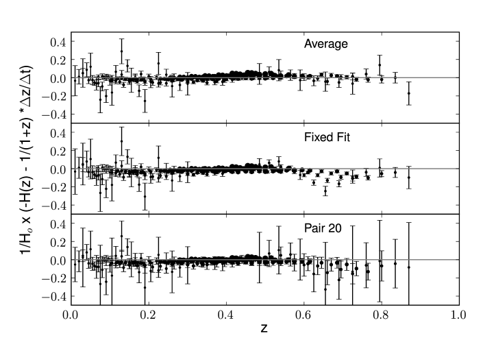
In Fig. 6, we present estimates of according to various methods. We plot the difference between our calculated value, , and the expected value for based on equation (3) in Jimenez & Loeb (2002):
| (3) |
where is the equation of state parameter for the dark energy, and in a model of de Lucia et al. (2006), .
The average method (top panel) recovers over a range of redshifts reasonable well. If we assume an error in the mean age at a specific redshift of 0.03 Gyr (this error will be discussed in §5), then can be calculated to a precision of at (using the redshift interval between and ). As can be seen in equation (2), the error in goes as the inverse of the difference in age: the closer the redshift bins, the larger the error. Between and , a small, systematic error in the mean age of as little as will result in the calculation of to be off by . Because of the small curvature of over these redshift ranges, large values in do not introduce a systematic difference in the value of .
The middle panel presents the results for fitting the distribution of ages to a function and determining a characteristic age. This is akin to fitting the envelope of oldest galaxies as in Jimenez et al. (2003). The data were fitted to the following function:
| (4) |
where,
| (5) |
For the first test, we allowed , , and to be free parameters along with . In the second test, we set and , which were the average parameters found during the free fits, and solved for from the best fit value of . The results for between the free and fixed fits were very similar and Fig. 6 (middle panel) shows the results for the fixed fit. Unlike the average estimate, is slightly underestimated at the highest redshifts. This is probably a result of the fitting function in equation (4) not fitting the normalized age distribution at higher redshifts well. At , can be calculated to by using our full sample at .
Finally, we calculate the value of at a given redshift based on the distribution of calculated between each pair of galaxies in the different redshift bins. If we used the entire sample, overlap between the age distributions significantly skews the results. Less than 10 galaxies results in anomalous values of . Using the 20 oldest galaxies minimizes both the systematic and random errors on the calculation of , however the results are not substantially different for using the 1000 oldest galaxies. Once we have calculated the value of from all of the pairs, at a given redshift is the three-sigma clipped mean of the distribution. The error is then given by the standard deviation of the sigma-clipped distribution. The estimate at high redshifts is also slightly below the model, but well within the errors. At , can be calculated to
It is reassuring that we can recover at a a single redshift using various metrics for the characteristic age of the population. Even the very gross estimate of the mean of the distribution provides very high accuracy () on the calculation of . Obviously using the ages from the MS is a best case scenario where the galaxy ages are determined without any error. In the next section, we explore the errors associated with age-dating LRGs.
4 Modelling and Age-Dating LRG spectra
There are a number of stellar population synthesis codes available which can be used to generate synthetic spectra once a star formation history has been determined (e.g. Fioc and Rocca-Volmerange 1997, Bruzual & Charlot 2003). However, the underlying physics is not always well understood: thermally-pulsating AGB stars may not be correctly modelled which effects infrared magnitudes significantly (Maraston 2005); an evolving Initial Mass Function (IMF) might be required to model cluster red-sequence galaxies which include many LRGs (van Dokkum 2008); related to the IMF, the alpha-element enhancement of old galaxies is not correctly modelled (Walcher et al. 2009); and, finally, dust modelling remains uncertain. Newer generations of models are currently being developed and tested (e.g. Maraston 2005, Conroy et al. 2009) along with improvements in the underlying stellar evolution models (Marigo et al. 2008). In addition, there is also uncertainty in the best method for deriving accurate ages both at low redshift (Kannappan & Gawiser 2007, Wolf et al. 2007, Trager & Somerville 2009) and at high redshift (Longhetti & Saracco 2009, Maraston et al. 2009, Muzzin et al. 2009). Unfortunately, the focus in these studies is more on broad-band and low-resolution spectra rather than the high-resolution, high-signal to noise (SNR) spectra we expect to need.
In this paper, we carry out a simple study of the age-dating question and leave a detailed discussion for the companion paper, including a comparison of different population synthesis models, age-dating techniques, and comments on IMF evolution, alpha-element enhancement and the role of AGB stars.
4.1 Modelling LRG Spectra
We build synthetic spectra of LRGs by combining single stellar population (SSP) spectral libraries of BC2003. The libraries are tabulated at ages ranging from years to years at a resolution of 3 Å across the whole wavelength range from 3200 to 9500 Å for a wide range of metallicities ( to ). Spectral coverage over a larger wavelength range, from 91 Å to 160 is also available but at lower resolution. For our studies here we have assumed the standard Salpeter initial mass function, with mass cut-offs at 0.1 and 100 . We refer the reader to BC2003 for details about the stellar evolution prescription used in constructing their libraries.
From the semi-analytic models of galaxy evolution based on the MS, one can extract both the star formation rate and metallicity of the cold gas out of which the stars are formed, as a function of time. Using these and the BC2003 SSP spectral libraries as input we calculate the emergent spectrum according to
| (6) |
In this equation, is the emergent spectrum in the rest frame; , the look-back time from the redshift of interest; , the look-back time at the start of formation’ , the star formation rate per unit mass per unit time; , the spectrum of an SSP as a function of age; and metallicity normalized to unit mass of stars and is the metallicity as a function of look back time. We ignore the effects of dust, since these LRGs are assumed to be devoid of any remaining gas and dust (Barber et al. 2007).
We generate spectra for all 1705, 1491, 1448, and 1337 galaxies selected from the MS at . In particular, we use the galaxies to examine the limitations in age dating the stellar populations.
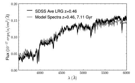
We used the revised colour-magnitude cuts discussed in §2.2 to extract a sample of galaxies from the SDSS catalogue (Abazajian et al. 2009). In Fig. 7, we present the average spectrum of the first 200 galaxies that match our cuts. For comparison, we plot the best fit model spectrum at . The fit was made from 3500-6000 Å, which includes only the high-resolution portion of the models. The best fit model has a mass-weighted age of Gyrs. The overall shape of the model is in good agreement with the observed spectrum although there are some inconsistencies at the edges.
4.2 Age-dating simulated LRG spectra with SSPs
In our first attempt to age-date simulated LRGs, we determine the ages for the 1448 model galaxies at using the SSP template library. For each source, we fit the full spectrum from Å using the SSP library described in §4. We do not add any flux errors or noise to the spectra and determine the best fit by minimizing the .
For our entire sample, the systematic and random errors from fitting the SSPs are listed in Table 2 as a function of redshift. It is not surprising to find a systematic error in the age determination using SSPs as compared to the mass-weighted age as the most appropriate comparison would be to the light-weighted age. Trager & Somerville (2009) perform a similar comparison for red galaxies in the Coma cluster comparing observed and simulated populations with SSPs. They also find that the SSPs underestimate the age of the galaxies and the SSP age is poorly correlated with the mass-weighted age due to recent star formation dominating the spectra. We also find that the offset in the systematic error does not correlate with the age of the Universe. The differential ages are less sensitive to systematic errors (Jimenez et al. 2004), and if the systematic errors were constant, this would not affect the calculation of . Since the bias does change with redshift, this prevents SSP-determined ages from being very useful for determining .
Based on the sample from McCarthy et al. (2004) of early type galaxies, Simon et al. (2005) claim they are well fit by a single burst population and use these ages to recover a value of . This is consistent with our results presented here as the resolution of their spectroscopic data ( Å) and the precision on are much greater than those that we examine here. McCarthy et al. (2004) do fit a majority of their objects with burst of less than 0.1 Gyrs, but the objects have a range of ages and formation redshifts that vary as much as 3 Gyrs. This is consistent with SSP fitting being dominated by the most recent star formation.
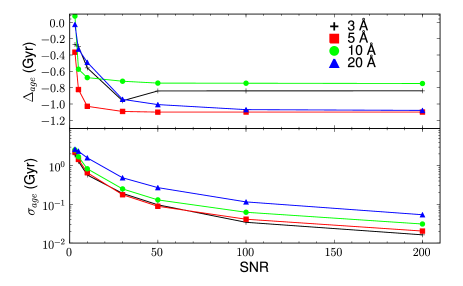
To explore the SSP fitting in more detail and to gain insight into the effects of changing the SNR and resolution of spectra, we performed Monte Carlo simulations for a subset of 10 galaxies. We selected ten random model galaxy spectra from our sample at . The template library and the spectra were convolved to a resolution of Å. Noise was added to each spectrum to give a range of signal to noise from . The SNR is here defined as the average SNR per resolution element of the spectrum between 3000 and 9000 Å, assuming simple shot noise. minimization was used to find the metallicity, age and normalization of the best fitting SSP spectrum. For each galaxy, this process was repeated 1000 times. Fig. 8 shows the average of the results from these simulations. As an example of the typical spread in ages, at a value of and Å, the minimum and maximum values for the ten galaxies were Gyrs and Gyrs .
The precision in this method, even when using the SSP, improves with increasing SNR as expected, and this method can very reliably reproduce the same age at high SNR for all resolutions. The random error on the age does decrease for smaller resolutions allowing for a better determination of the age. However, the poor accuracy of SSPs is again highlighted in Fig. 8. The mean offset in age seems to settle at a given value at , but it does not seem to be a monotonic function of the spectral resolution.
The accuracy of the age-dating is clearly critical for calculating . Unless systematic biases are constant with redshift and can be subtracted out or are well behaved and can be removed with modelling, they will contribute a significant systematic error to the age calculation. Even in this relatively straight forward simulation of using model galaxies from the MS, the SSPs are not able to reproduce the age without significant bias and are thus not adequate for the cosmic chronometer method.
| SSP Fit | Model Fit | ||||||
| z | Age222Age of the Universe in Gyrs. | Age | 333Mean difference between measured age and mass-weighted age. | 444 Standard deviation of difference between measured age and mass-weighted age. | Age | b | c |
| 0.32 | 10.08 | 8.15 | 0.14 | 1.85 | 8.32 | 0.01 | 0.29 |
| 0.46 | 8.95 | 7.42 | 0.20 | 1.72 | 7.22 | 0.01 | 0.33 |
| 0.51 | 8.59 | 7.06 | 0.23 | 1.65 | 6.83 | 0.02 | 0.33 |
| 0.56 | 8.25 | 6.62 | 0.16 | 1.69 | 6.48 | 0.01 | 0.33 |
4.3 Age-dating LRGs with model spectra
The large model library of different LRGs that we have created provide a mapping from spectra to mass-weighted ages. We can potentially use these spectra as our templates instead of the SSP templates. To test this, we extracted one spectrum from the models and then used the remaining models to age date that spectrum. Then, we repeated this for all of the other spectra. For each spectrum, we used its mass weighted age as its fiducial age. Testing the entire sample for 1448 model galaxies, we find a difference between the mass-weighted age and the measured age of Gyr with a dispersion of Gyrs. The result for the other redshifts are listed in Table 2. The systematic error, , and dispersion, , have been substantially reduced as compared to using SSPs. In addition, these ages can be used to measure because they have very small, regular bias with respect to the age of the Universe.
5 An Observing Program
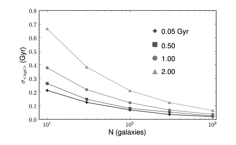
In this section, we explore the minimum observing time required to recover to a precision of , and at . Table 2 indicates that uncertainties on individual ages of galaxies could be as low as 0.3 Gyr if suitable templates can be used. However, since it is still unclear what the uncertainty on individual ages of galaxies will be in a realistic experiment, we explore observing requirements for four values of this uncertainty (0.05 Gyr, 0.5 Gyr, 1 Gyr and 2 Gyr). We consider observations at two redshifts: and , giving a redshift interval of . To simplify our estimate, the mean ages at the two redshifts are calculated using the average age of LRGs at each redshift (the first method discussed in §3). According to equation (2), the uncertainty on the mean ages will have to be Gyr to measure with precision.
To estimate the uncertainty in mean age as a function of the number of galaxies and the uncertainty on individual ages, we do a simple Monte Carlo simulation. We assume the uncertainty on individual galaxy ages are normally distributed, and the galaxy ages are drawn from the probability distribution for galaxies at given by the fit to equation (4) to the normalized age distribution. For each N, the simulation is repeated 1000 times and the standard deviation in the mean age is calculated. The results are presented in Fig. 9 and are used to calculate the total number of galaxies required to reach our desired precision.
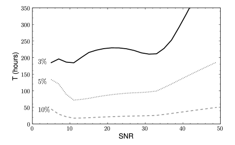
The other constraint on the total observing time is the exposure time per galaxy. We assume that we are only able to measure one galaxy at a time but note that multi-object spectroscopy could be used. In Fig. 8, the SNR for different spectral resolutions was presented. Even though the results in Fig. 8 are obtained using SSP fitting, we use them to provide a crude estimate of the resolution and signal to noise required to derive the random error on the ages of individual galaxies. In Fig. 10, we plot the total time needed as a function of signal to noise to calculate with different precision using the Robert Stobie Spectrograph (RSS, Kobulnicky et al. 2003) on the Southern African Large Telescope. We estimate that a 10% measurement is feasible using less than 20 hours of observing time but that a 3% measurement could require hours, even with our fairly optimistic estimates of .
We note however, that the RSS can be used in multi-object mode and, depending on the clustering, several LRGs may be expected in each field of view. Using our cuts, we estimate the space density of LRGs to be from the SDSS (without considering the effects of incompleteness), which is comparable to the value of from the MS. If we are able to observe two additional LRGs per set-up with while calculating to as outlined above, it would give us a sufficient numbers of LRGs to calculate to at redshifts between . This would put a far tighter constraint on the value of than measuring it from two redshift bins alone.
6 Conclusions
In this paper, we have shown that within the self-consistent Universe of the Millennium Simulation that Luminous Red Galaxies, when selected in an appropriate manner, can be used as cosmic chronometers. By selecting the galaxies from their rest-frame properties, we find that we can create a more homogeneous sample of objects than the apparent magnitude cuts used by Eisenstein et al. (2001). For galaxies at , we find that cuts of and select a sample of galaxies with similar star formation histories and formation redshifts in the MS.
The galaxies selected in our final cut do show very similar star formation histories with very few of the galaxies showing any star formation since . The ages also show something akin to downsizing (Cowie et al. 1996): the oldest galaxies are in the most massive halos. The distribution of the ages are very similar with each showing a small tail towards younger age, but with the very strong peak at a single age.
However we do note limitations in the use of the models of de Lucia et al. (2006). They are able to reproduce some of the major trends seen in local galaxy populations and seem to have similar number density as the SDSS out to . However, the model does have some limitations in reproducing some of the observed properties of LRGs while alternative models produce equally acceptable fits to the data. One such model explored here (Bower et al. 2006) was unsatisfactory in matching the observed number density of LRGs defined by an absolute magnitude cut at a .
Even though these galaxies have extended SFHs, they can be used as cosmic chronometers to recover the cosmology used in the MS. Using only galaxies selected from two redshifts, can be calculated to a precision of less than using three different methods. All three methods (averaging the ages, calculating a fit to the distribution, and comparing the ages of pairs of galaxies) were able to recover the cosmology used in de Lucia et al. (2006).
In §4, we showed that SSPs were not sufficient to accurately recover the ages for individual galaxies, which has also been shown for other samples (Maraston et al. 2009, Trager & Somerville 2009). Despite the relatively simple nature of the SFHs in Fig. 3, the calculated SSP ages were dominated by the most recent burst of star formation. If we use the average star formation history from the MS, we are able to replicate the properties of the model spectra, but in the next paper, we look in far greater detail at the modelling and fitting of LRG spectra. However, the semi-analytic models likely overestimate the extent of star formation in LRGs, and SSP models may provide better fits than indicated here.
Finally, we estimated the required time to complete the project using RSS on SALT. If systematics in the age can be controlled, at can be calculated to in a total of hours, which includes observing overheads. It is likely that tighter constraints could be put on the evolution of with additional data that could be obtained while making these observations. In addition to constraining , it would contribute a wealth of detailed information about the evolution of the most massive galaxies at intermediate redshift.
Throughout this work, we have highlighted a number of assumptions that we have made. Even with our refined selection, the star formation histories of these galaxies are not perfectly homogeneous as assumed by Jimenez & Loeb (2002), but can still be calculated to an accuracy better than . Other improvements on the measurement can be made by selecting a larger or more homogeneous sample as done by Stern et al. (2010). Uncertainties in the star formation history of simulated galaxies introduce far smaller errors than the contribution associated with age-dating the galaxies. In our next paper, we explore age-dating in more detail and note that increased uncertainties resulting from age-dating may lead to increased observing requirements.
Acknowledgments
We wish to thank Bruce Bassett for the original inspiration for this paper and for hosting the SA Cosmo Workshop, where the work begun in earnest. We greatly appreciate the constructive criticism received from our referee. SMC acknowledges SAAO and the NRF for support during this project, AR and CC acknowledges the South African SKA project, National Research Foundation (South Africa) and Centre for High Performance Computing for financial support. The Millennium Simulation databases used in this paper and the web application providing online access to them were constructed as part of the activities of the German Astrophysical Virtual Observatory. We acknowledge use of the Sloan Digital Sky Survey (SDSS and SDSS-II; see //www.sdss.org/ for funding, management, and participating institutions).
References
- Abazajian et al. (2009) Abazajian, K. N., et al. 2009, ApJS, 182, 543
- Almeida et al. (2008) Almeida, C., Baugh, C. M., Wake, D. A., Lacey, C. G., Benson, A. J., Bower, R. G., & Pimbblet, K. 2008, MNRAS, 386, 2145
- Barber et al. (2007) Barber, T., Meiksin, A., & Murphy, T. 2007, MNRAS, 377, 787
- Baugh et al. (2005) Baugh, C. M., Lacey, C. G., Frenk, C. S., Granato, G. L., Silva, L., Bressan, A., Benson, A. J., & Cole, S. 2005, MNRAS, 356, 1191
- Bower et al. (2006) Bower, R. G., Benson, A. J., Malbon, R., Helly, J. C., Frenk, C. S., Baugh, C. M., Cole, S., & Lacey, C. G. 2006, MNRAS, 370, 645
- Bruzual & Charlot (2003) Bruzual, G., & Charlot, S. 2003, MNRAS, 344, 1000
- Cannon et al. (2006) Cannon, R., et al. 2006, MNRAS, 372, 425
- Capozziello et al. (2004) Capozziello, S., Cardone, V. F., Funaro, M., & Andreon, S. 2004, PhRvD, 70, 123501
- Collins et al. (2009) Collins, C. A., et al. 2009, Nat, 458, 603
- Conroy et al. (2009) Conroy, C., Gunn, J. E., & White, M. 2009, ApJ, 699, 486
- Cowie et al. (1996) Cowie, L. L., Songaila, A., Hu, E. M., & Cohen, J. G. 1996, AJ, 112, 839
- Croton et al. (2006) Croton, D. J., et al. 2006, MNRAS, 365, 11
- Dantas et al. (2007) Dantas, M. A., Alcaniz, J. S., Jain, D., & Dev, A. 2007, A&A, 467, 421
- De Lucia et al. (2006) De Lucia, G., Springel, V., White, S. D. M., Croton, D., & Kauffmann, G. 2006, MNRAS, 366, 499
- Eisenstein et al. (2001) Eisenstein, D. J., et al. 2001, AJ, 122, 2267
- Ferreras et al. (2001) Ferreras, I., Melchiorri, A., & Silk, J. 2001, MNRAS, 327, L47
- Ferreras et al. (2003) Ferreras, I., Melchiorri, A., & Tocchini-Valentini, D. 2003, MNRAS, 344, 257
- Fioc & Rocca-Volmerange (1997) Fioc, M., & Rocca-Volmerange, B. 1997, A&A, 326, 950
- González et al. (2009) González, J. E., Lacey, C. G., Baugh, C. M., Frenk, C. S., & Benson, A. J. 2009, MNRAS, 397, 1254
- Jimenez & Loeb (2002) Jimenez, R., & Loeb, A. 2002, ApJ, 573, 37
- Jimenez et al. (2004) Jimenez, R., MacDonald, J., Dunlop, J. S., Padoan, P., & Peacock, J. A. 2004, MNRAS, 349, 240
- Jimenez et al. (2003) Jimenez, R., Verde, L., Treu, T., & Stern, D. 2003, ApJ, 593, 622
- Kannappan & Gawiser (2007) Kannappan, S. J., & Gawiser, E. 2007, ApJL, 657, L5 bibitem[Kereš et al.(2009)]2009MNRAS.395..160K Kereš, D., Katz, N., Fardal, M., Davé, R., & Weinberg, D. H. 2009, MNRAS, 395, 160
- Kobulnicky et al. (2003) Kobulnicky, H. A., Nordsieck, K. H., Burgh, E. B., Smith, M. P., Percival, J. W., Williams, T. B., & O’Donoghue, D. 2003, Proc. SPIE, 4841, 1634
- Longhetti & Saracco (2009) Longhetti, M., & Saracco, P. 2009, MNRAS, 394, 774
- Maraston (2005) Maraston, C. 2005, MNRAS, 362, 799
- Maraston et al. (2009) Maraston, C., Strömbäck, G., Thomas, D., Wake, D. A., & Nichol, R. C. 2009, MNRAS, 394, L107
- Marigo et al. (2008) Marigo, P., Girardi, L., Bressan, A., Groenewegen, M. A. T., Silva, L., & Granato, G. L. 2008, A&A, 482, 883
- Masjedi et al. (2008) Masjedi, M., Hogg, D. W., & Blanton, M. R. 2008, ApJ, 679, 260
- McCarthy et al. (2004) McCarthy, P. J., et al. 2004, ApJL, 614, L9
- Muzzin et al. (2009) Muzzin, A., Marchesini, D., van Dokkum, P. G., Labbé, I., Kriek, M., & Franx, M. 2009, arXiv:0906.2012
- Roseboom et al. (2006) Roseboom, I. G., et al. 2006, MNRAS, 373, 349
- Samushia et al. (2009) Samushia, L., Dev, A., Jain, D., & Ratra, B. 2009, arXiv:0906.2734
- Simon et al. (2005) Simon, J., Verde, L., & Jimenez, R. 2005, PhRvD, 71, 123001
- Springel et al. (2005) Springel, V., et al. 2005, Nat, 435, 629
- Stern et al. (2010) Stern, D., Jimenez, R., Verde, L., Kamionkowski, M., & Stanford, S. A. 2010, Journal of Cosmology and Astro-Particle Physics, 2, 8
- Trager & Somerville (2009) Trager, S. C., & Somerville, R. S. 2009, MNRAS, 395, 608
- Verkhodanov et al. (2005) Verkhodanov, O. V., Parijskij, Y. N., & Starobinsky, A. A. 2005, Bull. Special Astrophys. Obs., 58, 5
- van Dokkum (2008) van Dokkum, P. G. 2008, ApJ, 674, 29
- Wake et al. (2006) Wake, D. A., et al. 2006, MNRAS, 372, 537
- Wake et al. (2008) Wake, D. A., et al. 2008, MNRAS, 387, 1045
- Walcher et al. (2009) Walcher, C. J., Coelho, P., Gallazzi, A., & Charlot, S. 2009, arXiv:0906.5000
- Wolf et al. (2007) Wolf, M. J., Drory, N., Gebhardt, K., & Hill, G. J. 2007, ApJ, 655, 179
- York et al. (2000) York, D. G., et al. 2000, AJ, 120, 1579