CMB Constraints on Primordial non-Gaussianity from the Bispectrum ($f_{\rm NL}$) and Trispectrum ($g_{\rm NL}$ and $\tau_{\rm NL}$) and a New Consistency Test of Single-Field Inflation

Abstract

We outline the expected constraints on non-Gaussianity from the cosmic microwave background (CMB) with current and future experiments, focusing on both the third ($f_{\rm NL}$) and fourth-order ($g_{\rm NL}$ and $\tau_{\rm NL}$) amplitudes of the local configuration or non-Gaussianity. The experimental focus is the skewness (two-to-one) and kurtosis (two-to-two and three-to-one) power spectra from weighted maps. In adition to a measurement of $\tau_{\rm NL}$ and $g_{\rm NL}$ with WMAP 5-year data, our study provides the first forecasts for future constraints on $g_{\rm NL}$. We describe how these statistics can be corrected for the mask and cut-sky through a window function, bypassing the need to compute linear terms that were introduced for the previous-generation non-Gaussianity statistics, such as the skewness estimator. We discus the ratio $A_{\rm NL}=\tau_{\rm NL}/(6f_{\rm NL}/5)^{2}$ as an additional test of single-field inflationary models and discuss the physical significance of each statistic. Using these estimators with WMAP 5-Year V+W-band data out to $l_{\rm max}=600$ we constrain the cubic order non-Gaussianity parameters $\tau_{\rm NL}$, and $g_{\rm NL}$ and find $-7.4<g_{\rm NL}/10^{5}<8.2$ and $-0.6<\tau_{\rm NL}/10^{4}<3.3$ improving the previous COBE-based limit on $\tau_{\rm NL}<10^{8}$ nearly four orders of magnitude with WMAP.

I Introduction

We have now entered an exciting time in cosmological studies where we are now beginning to constrain simple slow-roll inflationary models with high precision observations of the cosmic microwave background (CMB) and large-scale structure. In addition to constraining inflationary model parameter space with traditional parameters such as the spectral index $n_{s}$ and the tensor-to-scalar ratio $r$, we may soon be able to use parameters associated with primordial non-Gaussianity to improve model selection.

In the simplest realistic inflationary models, the field(s) responsible for inflation have minimal interactions. Such an interaction-less situation should have led to Gaussian primordial curvature perturbations, assuming that pertubations in the inflaton field generates the curvature perturbation. In this case, the two point correlation function contains all the informations on these perturbations. If the early inflation field(s) have non-trivial interactions, higher-order correlation functions of the curvature perturbations will contain connected pieces encoding information about the primordial inflationary interactions. This is analogous to the situation encountered in particle physics where correlation functions can be separated into unconnected and connected Feynman diagrams, the later containing information about the underlying interactions (see Fig. 1 for an example involving the four-point function). A detection of non-Gaussianity therefore gives an important window into the nature of the inflation field(s) and their interactions.

To parameterize the non-Gaussianity of a nearly Gaussian field, such as the primordial curvature perturbations $\zeta({\bf x})$, we can expand them perturbatively Kogo:2006kh to second order as:

$$\zeta({\bf x})=\zeta_{g}({\bf x})+{3\over 5}f_{\rm NL}\left[\zeta_{g}^{2}({\bf x})-\langle\zeta^{2}_{g}({\bf x})\rangle\right]+{9\over 25}g_{\rm NL}\zeta_{g}^{3}({\bf x}),$$ (1)

where $\zeta_{g}({\bf x})$ is the purely Gaussian part with $f_{\rm NL}$ and $g_{\rm NL}$ parametrizing the first and second order deviations from Gaussianity. This parameterization of the curvature perturbations is known as the local model as this definition is local in space.

Much effort has already gone into measuring non-Gaussianity at first-order in curvature perturbations using the bispectrum of the CMB anisotropies or large-scale structure galaxy distribution parametrerized by $f_{\rm NL}$ (see Eq. 1). These studies have found $f_{\rm NL}$ to be consistent with zero Yadav:2007yy ; Smith:2009jr ; Komatsu:2010fb ; Smidt:2009ir . However, there is hope that a significant detection may be possible by future surveys that will lead to improved errors Komatsu:2009kd .

Figure 1: Four point correlation function for the $\phi^{3}$ theory. The correlation functions breaks up into interaction-less unconnected diagrams and connected diagrams containing information about the interactions.

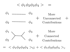
In the trispectrum, two parameters of second-order non-Gaussianity at fourth-order in curvature perturbations, $\tau_{\rm NL}$ and $g_{\rm NL}$, can be measured. In this paper we also introduce a third parameter, $A_{\rm NL}$ is an additional parameter that compares $\tau_{\rm NL}$ of the trispectrum to $(6f_{\rm NL}/5)^{2}$ from the bispectrum as a ratio:

$$A_{\rm NL}={\tau_{\rm NL}\over(6f_{\rm NL}/5)^{2}}.$$ (2)

This ratio can be quite different for many inflationary models Byrnes:2010em ; Chen:2009bc and, as will be shown below, $A_{\rm NL}\neq 1$ rules out single-field inflationary models altogether, including the standard curvaton scenario (which neglects perturbations from the inflaton field).

In this paper we discuss the skewness and kurtosis power spectra method for probing primordial non-Gaussianity and give constraints for the first ($f_{\rm NL}$) and second-order ($g_{\rm NL}$ and $\tau_{\rm NL}$) amplitudes of the local model in addition to their ratio $A_{\rm NL}$. Using the bispectrum of CMB anisotropies as seen by WMAP 5-year data, Smidt et al. (2009) found $-36.4<f_{\rm NL}<58.4$ at 95% confidence Smidt:2009ir . This is to be compared with the most recent WMAP 7 measurement of $-10<f_{\rm NL}<74$ Komatsu:2010fb , where part of the discrepancy is due to a difference in optimization Smith . As outlined in Section VI, using the trispectrum of the same data we find that $-0.6<\tau_{\rm NL}/10^{4}<3.3$ and $-7.4<g_{\rm NL}/10^{5}<8.2$ at 95% confidence level showing second order non-Gaussianity is consistent with zero in WMAP. This paper serves as a guide to the analysis process behind our derived limits on $\tau_{\rm NL}$, $g_{\rm NL}$ and $A_{\rm NL}$.

Furthermore, in this paper we analyze what to realistically expect when measuring non-Gaussianity from CMB temperature data. We believe establishing what constraints can be placed upon $f_{\rm NL}$, $\tau_{\rm NL}$, $g_{\rm NL}$ and $A_{\rm NL}$ by future experiments is important in determining what models may and may not be tested by future data. We also highlight several advantages of our work, including ways to correct the cut-sky and mask through a window function without using linear terms which are computationally prohibative Creminelli:2005hu ; Yadav:2007ny .

This paper is organized as follows: In Section II we review how non-Gaussianity may be used to distinguish between common inflationary models and stress the physical significance of each statistic. In Section III we describe the skewness and kurtosis power spectra and explain how they may be used to extract information about primordial non-Gaussianity from the CMB. In Section IV, we describe the signal-to-noise of each estimator, how to add the experimental beam and noise to these calculations and discuss why these power spectra have the advantage for dealing with a cut sky. In Section V we calculate the fisher bounds for upcoming experiments for each statistic. In Section VI we discuss the technical details for measuring non-Gaussianity in the trispectrum and in Section VII we conclude with a discussion.

II Non-Gaussianity From Common Inflationary Models

Non-Gaussinity is a powerful tool that may be used to distinguish between inflationary models. The simplest models do not produce a detectable amount of non-Gaussianity. Maldacena Maldacena:2002vr has shown that a single-field, experiencing slow roll with canonical kinetic energy and an initial Bunch-Davies vacuum state produces

$$f_{\rm NL}={5\over 12}(n_{s}+f(k)n_{t}).$$ (3)

Here $n_{s}$ and $n_{t}$ are the scalar and tensor spectral indices respectively. The function $f(k)$ has a range $0\leq f(k)\leq{5\over 6}$ based on the triangle shapes (see below) of the $k_{i}$ such that $f=0$ in the squeezed limit and $f={5\over 6}$ for an equilateral triangle. For this reason, $f_{\rm NL}<1$ will remain undetectable in the simple slow roll scenario with CMB data alone.

Figure 2: Plot of the shape functions $S^{\rm local}(1,k_{2},k_{3})$ and $S^{\rm equil}(1,k_{2},k_{3})$ normalized such that $S(1,1,1)=1$. In these plots only values satisfying the triangle inequality $k_{2}+k_{3}\geq k_{1}=1$ as well as the requirement $k_{2}\leq k_{3}$ to prevent showing equivalent configurations are non-zero. The plot on top verified $S^{local}$ is maximized when $k_{1}\sim k_{3}\gg k_{2}$ whereas the bottom plot verifies $S^{equal}$ is maximised when $k_{1}\sim k_{2}\sim k_{3}$.

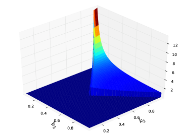
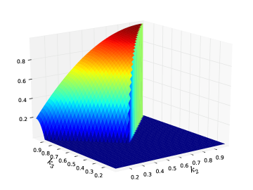
If any of the above assumptions are violated, very specific types of non-Gaussianity are produced Komatsu:2009kd ; Baumann:2009ds ; Komatsu:2010hc . In the bispectrum $B_{\zeta}(k_{1},k_{2},k_{3})$ defined by

$$\left<\zeta_{{\bf k}_{1}}\zeta_{{\bf k}_{2}}\zeta_{{\bf k}_{3}}\right>=(2\pi)^{3}\delta({\bf k}_{1}+{\bf k}_{2}+{\bf k}_{3})B_{\zeta}(k_{1},k_{2},k_{3}),$$ (4)

where $\zeta$ is the primordial curvature perturbation, non-Gaussianities show up as triangles in Fourier space. Different triangle shapes are be produced by different underlying physics, for example:

• squeezed triangle ($k_{1}\sim k_{2}\gg k_{3}$) This is the dominating shape from multi-field, curvaton, inhomogeneous reheating and Ekpyrotic models.

• equilateral triangle ($k_{1}=k_{2}=k_{3}$) This shape is produced by non-canonical kinetic energy with higher derivative interactions and non-trivial speeds of sound.

• folded triangle ($k_{1}=2k_{2}=2k_{3}$) These triangles are produced by non-adiabatic-vacuum models.

Additionally, linear combinations of the above shapes or intermediate cases such as elongated triangles ($k_{1}=k_{2}+k_{3}$) and isosceles triangles ($k_{1}>k_{2}=k_{3}$) are possible Komatsu:2009kd ; Baumann:2009ds ; Komatsu:2010hc . The most recent WMAP 7 constraints on the amount of non-Gaussinaity from each shape is $-10<f^{\rm local}_{\rm NL}<74$, $-214<f^{\rm equil}_{\rm NL}<266$ and $-410<f^{\rm orthog}_{\rm NL}<6$ at 95% confidence Komatsu:2010fb .

A convenient way to distinguish between shapes is to introduce the shape function defined as

$$S(k_{1},k_{2},k_{3})\equiv{1\over N}(k_{1}k_{2}k_{3})^{2}B_{\zeta}(k_{1},k_{2},k_{3}),$$ (5)

where N is a normalization factor often taken to be $1/f_{\rm NL}$. Using a notation introduced by Fergusson and Shellard Fergusson , we can give the shape function for the more common configurations as:

$$S^{\rm local}(k_{1},k_{2},k_{3}) \propto {K_{3}\over K_{111}},$$ (6)

$$S^{\rm equil}(k_{1},k_{2},k_{3}) \propto {\tilde{k}_{1}\tilde{k}_{2}\tilde{k}_{3}\over K_{111}},$$ (7)

$$S^{\rm folded}(k_{1},k_{2},k_{3}) \propto {1\over K_{111}}(K_{12}-K_{3})+4{K_{2}\over\tilde{k}_{1}\tilde{k}_{2}\tilde{k}_{3}},$$ (8)

where

$$K_{p} = \sum_{i}(k_{i})^{p}\ \ \ {\rm with}\ \ \ K=K_{1},$$ (9)

$$K_{pq} = {1\over\Delta_{pq}}\sum_{i\neq j}(k_{i})^{p}(k_{j})^{q},$$ (10)

$$K_{pqr} = {1\over\Delta_{pqr}}\sum_{i\neq j\neq l}(k_{i})^{p}(k_{j})^{q}(k_{l})^{r},$$ (11)

$$\tilde{k}_{ip} = K_{p}-2(k_{i})^{p}\ \ \ {\rm with}\ \ \ \tilde{k}_{i}=\tilde{k}_{i1},$$ (12)

with $\Delta_{pq}=1+\delta_{pq}$ and $\Delta_{pqr}=\Delta_{pq}(\Delta_{qr}+\delta_{pr})$ (no summation). Plots for the local and equilateral shapes are given in Figure 2.

In addition to $f_{\rm NL}$ being generated by different shapes, it also may vary with scale. Recently, a new parameter has been introduced to measure this scale dependance defined as:

$$n_{f_{\rm NL}}(k)={d\ln{\left|f_{\rm NL}(k)\right|}\over d\ln k}.$$ (13)

This scale dependance has the ability to test the ansatz 1 to test whether the local model should allow for $f_{\rm NL}$ to vary with scale Byrnes:2009pe . Using the results of Smidt et al.(2009) (Fig. 16 of Ref Smidt:2009ir ) and assuming

$$f_{\rm NL}(l)=f_{\rm NL_{200}}\left({l\over l_{200}}\right)^{n_{f_{\rm NL}}(l)},$$ (14)

we can constrain $n_{f_{\rm NL}}(l)$ to roughly $-2.5<n_{f_{\rm NL}}(l)<2.3$ at 95% confidence. We therefore find $f_{\rm NL}$ is consistent with having no scale dependance.

In this paper we focus on the local model that probes non-Gaussianty of a squeezed shape. As mentioned above, simple inflationary models can not produce a detectable amount of non-Gaussinity for local models. We now review the prediction for local non-Gaussianity for the most common models.

II.1 Review Of The $\delta N$ formalism.

The curvature perturbation can be conveniently described using the $\delta N$ formalism Starobinsky:1982ee ; Starobinsky:1986fxa ; Byrnes:2006vq ; Lyth:2005fi ; Suyama:2007bg . During inflation, spacetime expands by a certain number of e-folds N. By Heisenberg’s uncertainty principle, expansion for each point in space ends at slightly different times producing a spatially dependent total e-fold:

$$N(x)=\int_{t_{i}}^{t^{f}}H(x,t)dt,$$ (15)

where $H(x,t)$ is the Hubble parameter allowing us to define $N(x)={\bar{N}}+\delta N(x)$. The fluctuations in e-fold about the mean value ${\bar{N}}$, which correspond to perturbations in local expansion, are the curvature perturbations $\zeta=\delta N$.

In addition to a spatial parameterization, we may parameterize the number of e-folds by the underlying fields $\zeta=N(\phi^{A})-{\bar{N}}$ where $\phi^{A}$ represents the initial values for the scalar fields . If we write out the fields as $\phi^{A}={\bar{\phi}}^{A}+\delta\phi^{A}$ we can expand the curvature perturbations as

$$\zeta=\delta N=\sum_{n}{1\over n!}N_{A_{1}A_{2}...A_{n}}\delta\varphi^{A_{1}}\delta\varphi^{A_{1}}...\delta\varphi^{A_{n}}.$$ (16)

The $N_{x}$ means the derivative of N with respect to the fields $x$. For example, $N_{A_{1}A_{2}}\equiv{\partial^{2}N\over\partial\varphi^{A_{1}}\partial\varphi^{A_{2}}}$. In this equation there is an implicit sum over the $A_{i}$. Einstein summation is implicit in all equations relating to the $\delta N$ formalism.

Using this formalism we may compute to first order from $\zeta=N_{A}\delta\varphi^{A}$:

$$\left<\zeta_{\bf k}\zeta_{\bf k^{\prime}}\right> = N_{A}N_{B}C^{AB}(k)(2\pi)^{3}\delta^{3}({\bf k}+{\bf k^{\prime}}),$$ (17)

where $C^{AB}(k)$ in the slow roll limit becomes to leading order $\delta^{AB}P(k)$.

Likewise, we can calculate the bispectrum and trispectrum in this formalism;

$$B_{\zeta}(k_{1},k_{2},k_{3}) = N_{A}N_{BC}N_{D}[C^{AB}(k_{1})C^{BD}(k_{2})$$

$$+\ C^{AB}(k_{1})C^{BD}(k_{2})+C^{AB}(k_{1})C^{BD}(k_{2})],$$

$$T_{\zeta}(k_{1},k_{2},k_{3},k_{4}) = N_{A_{1}A_{2}}N_{B_{1}B_{2}}N_{C}N_{D}$$ (19)

$$\times[C^{A_{2}B_{2}}(k_{13}) C^{A_{1}C}(k_{2})C^{B_{1}D}(k_{2})+(11\;{\rm perms)}]$$

$$+N_{A_{1}A_{2}A_{3}}N_{B}N_{C}N_{D}$$

$$\times[C^{A_{1}B}(k_{13}) C^{A_{2}C}(k_{2})C^{A_{3}D}(k_{2})+(3{\rm\;perms)}],$$

where $k_{ij}=|{\bf k}_{i}+{\bf k}_{j}|$. In the slow roll limit to leading order these expressions may be rewritten as:

$$B_{\zeta}(k_{1},k_{2},k_{3}) = {6\over 5}f_{\rm NL}[P_{\zeta}(k_{1})P_{\zeta}(k_{2})+$$

$$P_{\zeta}(k_{2})P_{\zeta}(k_{3})+P_{\zeta}(k_{3})P_{\zeta}(k_{1})],$$

$$T(k_{1},k_{2},k_{3},k_{4}) = \tau_{\rm NL}[P_{\zeta}(k_{13})P_{\zeta}(k_{3})P_{\zeta}(k_{4})+(11\;{\rm perms)}]$$ (21)

$$+\ {54\over 25}g_{\rm NL}[P_{\zeta}(k_{2})P_{\zeta}(k_{3})P_{\zeta}(k_{4})+(3\;{\rm perms)}],$$

where $P_{\zeta}(k)=N_{A}N_{B}C^{AB}(k)$ and therefore in the slow roll limit $P_{\zeta}(k)=N_{A}N^{A}P(k)$.

From the above two expressions we can read off the values for each statistic:

$$f_{\rm NL} = {5\over 6}{N_{A}N_{B}N^{AB}\over\left(N_{C}N^{C}\right)^{2}};$$ (22)

$$\tau_{\rm NL} = {N_{AB}N^{AC}N^{B}N_{C}\over\left(N_{D}N^{D}\right)^{3}};$$ (23)

$$g_{\rm NL} = {25\over 54}{N_{ABC}N^{A}N^{B}N^{C}\over\left(N_{D}N^{D}\right)^{3}};$$ (24)

$$A_{\rm NL} = {\tau_{\rm NL}\over(6f_{\rm NL}/5)^{2}}.$$ (25)

II.2 General Single-Field Models

For a single scalar field $\varphi$ perturbing $N(\varphi)$ we may expand $\zeta$, using the above formalism Byrnes:2006vq , as:

$$\zeta=N^{\prime}\delta\varphi+{1\over 2}N^{\prime\prime}\delta\varphi^{2}+{1\over 6}N^{\prime\prime\prime}\delta\varphi^{3}+...,$$ (26)

where $N^{\prime}=dN/d\varphi$. Note that we do not require that $\varphi$ is the inflaton field, it could be the curvaton or a field which modulates the efficiency of reheating. From equations 22-24 we may immediately read off

$$f_{\rm NL} = {5\over 6}{N^{\prime\prime}\over\left(N^{\prime}\right)^{2}};$$ (27)

$$\tau_{\rm NL} = {\left(N^{\prime\prime}\right)^{2}\over\left(N^{\prime}\right)^{4}};$$ (28)

$$g_{\rm NL} = {25\over 54}{N^{\prime\prime\prime}\over\left(N^{\prime}\right)^{3}};$$ (29)

$$A_{\rm NL} = 1.$$ (30)

Equations 27 and 28 yield a very important consequence of single-field models namely $\tau_{\rm NL}=(6f_{\rm NL}/5)^{2}$. This is a general result and therefore $A_{\rm NL}\neq 1$ may be used to rule out single-field models all together.

II.3 Multi-Field Inflationary Models

Suyama and Yamaguchi showed in general $\tau_{\rm NL}\geq(6f_{\rm NL}/5)^{2}$ by the Cauchy-Schwartz inequality and equality only holds if $N_{A}$ is an eigenmode of $N_{AB}$ Suyama:2007bg . Models where equality does not hold can not be those of a single-field. We now examine such models.

Unlike the single-field case, using the $\delta N$ formalism to make general statements about multi-field models is nearly impossible. Instead, one is forced to work with specific models that utilize simplifying assumptions. We now present a class of multi-field models that we believe is sufficiently general to uncover many details that are characteristic of multi-field models in general.

Recently, Byrnes and Choi reviewed two field models with scalar fields $\varphi$ and $\chi$ that have a separable potential $W(\varphi,\chi)=U(\varphi)V(\chi)$ Byrnes:2010em ; Vernizzi:2006ve ; Choi:2007su ; Battefeld:2006sz ; Seery:2006js . The slow roll parameters for these models are:

$$\epsilon_{\varphi} = {M_{p}^{2}\over 2}\left({U_{,\varphi}\over U}\right)^{2},\;\epsilon_{\chi}={M_{p}^{2}\over 2}\left({V_{,\chi}\over V}\right)^{2},$$ (31)

$$\eta_{\varphi\varphi} = M_{p}^{2}{U_{,\varphi\varphi}\over U},\hskip 2.84544pt\eta_{\varphi\chi}=M_{p}^{2}{U_{,\varphi}V_{,\chi}\over W},\hskip 2.84544pt\eta_{\chi\chi}=M_{p}^{2}{V_{,\chi\chi}\over V},$$

from which we can define

$$\tilde{r}={\epsilon_{\chi}\over\epsilon_{\varphi}}e^{2(\eta_{\varphi\varphi}-\eta_{\chi\chi})N}.$$ (33)

For this class of models, in the regions where $|f_{NL}|>1$ we have

$$f_{\rm NL} = {5\over 6}\eta_{\chi\chi}{\tilde{r}\over(1+\tilde{r})^{2}}e^{2(\eta_{\varphi\varphi}-\eta_{\chi\chi})N};$$ (34)

$$g_{\rm NL} = {10\over 3}{\tilde{r}(\eta_{\varphi\varphi}-2\eta_{\chi\chi})-\eta_{\chi\chi}\over 1+\tilde{r}}f_{\rm NL};$$ (35)

$$\tau_{\rm NL} = {1+\tilde{r}\over\tilde{r}}\left({6f_{\rm NL}\over 5}\right)^{2};$$ (36)

$$A_{\rm NL} = {1+\tilde{r}\over\tilde{r}}.$$ (37)

It is worth noting that both $\tau_{\rm NL}$ and $g_{\rm NL}$ are related to $f_{\rm NL}$ for this class of models. Here we have $|g_{\rm NL}|<|f_{\rm NL}|$ which will therefore be much harder to detect. On the contrary, $\tau_{\rm NL}>(6f_{\rm NL}/5)^{2}$ so that non-Gaussinity may in fact be easier to detect in the trispectrum than the bispectrum for some multi-field models. Here we find $A_{\rm NL}={(1+\tilde{r})/\tilde{r}}>1$. The scale dependance of $f_{\rm NL}$ has also been worked out for this class of models and was found to be $n_{f_{\rm NL}}=-4(\eta_{\varphi\varphi}-\eta_{\chi\chi})/(1+\tilde{r})<0$.

II.4 Curvaton Models

In the curvaton scenario, a weakly interacting scalar field $\chi$ exists in conjunction to the inflaton $\varphi$ Enqvist:2009N ; Enqvist:2009T ; Byrnes:2010em ; Byrnes:2006vq ; Huang:2008bg ; Enqvist:2009ww . During inflation, the curvaton field is subdominant, but after inflation $\chi$ can dominate the energy density. The decay of the inhomogeneous curvation field in this scenario produces the curvature perturbations and not the inflaton.

If such a curvaton field is the soul contributor to curvature perturbations, we can write out the perturbations using the $\delta N$ formalism as we did in the single field case:

$$\zeta=N^{\prime}\delta\chi+{1\over 2}N^{\prime\prime}\delta\chi^{2}+{1\over 6}N^{\prime\prime\prime}\delta\chi^{3}+...,$$ (38)

where now $N^{\prime}=dN/d\chi$. Immediately we recover the relations 27-29 and find for such curvaton models $A_{\rm NL}=1$ as should be expected from curvature perturbations generated by a single-field.

Recently, curvation models with generic potentials of the form

$$V={1\over 2}m^{2}\chi^{2}+\lambda\chi^{n+4},$$ (39)

have been analyzed Huang:2008bg ; Enqvist:2009ww . Here $m$ is the curvaton’s mass and $\lambda$ is a coupling constant. For such models $N$ in Equation 38 has been worked out giving:

$$f_{\rm NL} = {5\over 4r_{\chi}}(1+h)-{5\over 3}-{5r_{\chi}\over 6},$$ (40)

$$g_{\rm NL} = {25\over 54}\Bigg{[}{9\over 4r_{\chi}^{2}}(\tilde{h}+3h)-{9\over r_{\chi}}(1+h)$$

$$+{1\over 2}(1-9h)+10r_{\chi}+3r_{\chi}^{2}\Bigg{]},$$

where

$$r_{\chi}={3\Omega_{\chi,D}\over 4-\Omega_{\chi,D}},\hskip 8.5359pth={\chi_{0}\chi_{0}^{\prime\prime}\over\chi_{0}^{\prime 2}},\hskip 8.5359pt\tilde{h}={\chi^{2}_{0}\chi_{0}^{\prime\prime\prime}\over\chi_{0}^{\prime 3}}.$$ (42)

Here $\Omega_{\chi,D}$ is the energy density at time of curvaton decay, $\chi_{0}$ is the curvation field during oscillations just before decay and the primes here denote derivatives with respect to time.

Unlike single scalar field inflation, curvaton models can have large self interactions. Enqvist et al. pointed out that even if $f_{\rm NL}$ is small, $g_{\rm NL}$ can be large for significant levels of self-interactions Enqvist:2009ww . This places a physical significance on $g_{\rm NL}$ that can be thought of as parameterizing large self-interactions.

II.5 Brief Summary

In this section we have discussed the physical significance of each statistic $f_{\rm NL}$, $g_{\rm NL}$, $\tau_{\rm NL}$ and $A_{\rm NL}$. In the bispectrum, $f_{\rm NL}$ receives contributions from different shaped triangles in Fourier space related to different underlying physics. By analyzing the amount of non-Gaussianity from these different shapes we can distinguish between models with multiple fields, non-canonical kinetic energy and non-adiabatic vacuums.

In addition we stressed the physical significance of local non-Gaussianity in the trispectrum. The relation $A_{\rm NL}=\tau_{\rm NL}/(6f_{\rm NL}/5)^{2}$ is an important constraint of multi-field models. A general result for single-field models is $A_{\rm NL}=1$. Lastly, $g_{\rm NL}$ will place important constraints on the level of self-interactions.

III Power Spectra Estimators For First and Second-Order Non-Gaussianity.

We would like to find a way to measure the non-Gaussianity of these fields from something directly observable. Fortunately, information about the curvature perturbations are contained within the CMB through the spherical harmonic coefficients of the temperature anisotropies:

$$a_{lm} = 4\pi(-i)^{l}\int\frac{d^{3}{\bf k}}{(2\pi)^{3}}\Phi({\bf k})g_{Tl}(k)Y_{l}^{m*}({\hat{\bf k}}),$$ (43)

$$\theta(\hat{\bf n}) = \frac{\delta T}{T}(\hat{\bf n})=\sum_{lm}a_{lm}Y_{l}^{m*}({\hat{\bf n}})\,,$$ (44)

where $\Phi({\bf k})$ are the primordial curvature perturbations, $g_{Tl}$ is the radiation transfer function that gives the angular power spectrum $C_{l}=(2/\pi)\int k^{2}dkP_{\Phi}(k)g^{2}_{{\rm T}l}(k)$, $\theta$ is the field of temperature fluctuations in the CMB and $Y^{l}_{m}$’s are the spherical harmonics. (In this equation, the curvature perturbation $\Phi$ is related to $\zeta$ through the relation $\Phi=(3/5)\zeta$.)

If the curvature perturbations are purely Gaussian, all the statistical information we can say about them is contained in the two point correlation function $\left<\Phi({\bf x_{1}})\Phi({\bf x_{2}})\right>$. The information contained in the two point function is usually extracted in spherical harmonic space, leading to the power spectrum $C_{l}$, defined by:

$$C_{l}=\left<a_{lm}a_{lm}\right>={1\over(2l+1)}\sum_{m}a_{lm}a^{*}_{lm}.$$ (45)

However, if the curvature perturbations are slightly non-Gaussian, this two point function is no longer sufficient to articulate all the information contained in the field. With non-Gaussianity, extra information can be extracted from the three, four and higher n-point correlation functions Komatsu:2009kd .

We now discuss estimators that can be used to measure non-Gaussianity at first and second order corresponding to the third and fourth-order in curvature perturbations respectively.

III.1 Skewness Power Spectrum Estimator for the Bispectrum.

In order to detect Gaussianity at first order, we must turn to the three point correlation function of the primordial curvature perturbations $\left<\Phi({\bf x_{1}})\Phi({\bf x_{2}})\Phi({\bf x_{3}})\right>$. As mentioned above, we can extract information from the curvature perturbations by analyzing the $a_{lm}$s of the CMB. The three point correlation function of the $a_{lm}$s is called the bispectrum can be decomposed as followsKomatsu:2002db :

$$\langle a_{lm}a_{l^{\prime}m^{\prime}}a_{l^{\prime\prime}m^{\prime\prime}}\rangle=B_{ll^{\prime}l^{\prime\prime}}\left(\begin{array}[]{ c c c }l&l^{\prime}&l^{\prime\prime}\\ m&m^{\prime}&m^{\prime\prime}\end{array}\right).$$ (48)

where

$$B_{ll^{\prime}l^{\prime\prime}}\equiv\sqrt{(2l+1)(2l^{\prime}+1)(2l^{\prime}+1)\over 4\pi}\left(\begin{array}[]{ c c c }l&l^{\prime}&l^{\prime\prime}\\ 0&0&0\end{array}\right)b_{ll^{\prime}l^{\prime\prime}}.$$ (51)

Here the symbols in parenthesis are called the Wigner-3j symbols and enforce rotational invariance of the CMB, as well as ensuring the proper triangle equality holds between $l$, $l^{\prime}$ and $l^{\prime\prime}$ namely: $|l_{i}-l_{j}|\leq l_{k}\leq|l_{i}+l_{j}|$ for any combination of $i$, $j$ and $k$. For more information on the wigner 3j symbols, the reader is directed to the appendix of Ref. Komatsu:2002db .

The quantity $b_{ll^{\prime}l^{\prime\prime}}$, known as the reduced bispectrum, encases all the other information in the bispectrum and for the local model can be computed analytically as:

$$b_{l_{1}l_{2}l_{3}}=2f_{NL}\int r^{2}dr\left[\alpha_{l_{1}}(r)\beta_{l_{2}}(r)\beta_{l_{3}}(r)+{\rm cyc.perm.}\right],$$ (52)

where

$$\alpha_{l}(r) \equiv {2\over\pi}\int_{0}^{\infty}k^{2}dkg_{Tl}(k)j_{l}(kr),$$

$$\beta_{l}(r) \equiv {2\over\pi}\int_{0}^{\infty}k^{2}dkP_{\Phi}(k)g_{Tl}(k)j_{l}(kr).$$ (53)

Here, $P_{\Phi}(k)\propto k^{n_{s}-4}$ is the primordial power spectrum of curvature perturbations, $g_{Tl}(k)$ is defined above, $j_{l}(kr)$ are the spherical Bessel functions and $r$ parameterizes the line of sight.

Figure 3: The top plot compares various $\beta(r)$ for different $\tau_{*}$ and the bottom is the same for $\alpha(r)$.

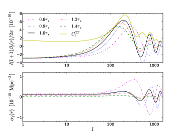
Traditionally, the non-Gaussianity parameter $f_{\rm NL}$ is given as a single number where the information from all the triangles configurations are collapsed into a single number called skewness ($S_{3}$) defined as

$$S_{3}\equiv\int r^{2}dr\int d{\bf{\hat{n}}}A(r,{\bf{\hat{n}}})B^{2}(r,{\bf{\hat{n}}}).$$ (54)

where $A(r,{\bf{\hat{n}}})$ and $B(r,{\bf{\hat{n}}})$, are defined below in equations 55 and 56. Recently, new techniques have been developed to measure $f_{\rm NL}$ from a power spectrum called the skewness power spectrum Cooray:2001ps ; Munshi:2009ik . These new estimators based on the analysis of power spectra are equivalent to $S_{3}$ in the limit of homogeneous noise Komatsu:2010fb but have certain advantages discussed at the bottom of this subsection. These advantages include the ability to separate foregrounds and other secondary non-Gaussian signals and the ability to correct for the cut-sky without having to compute so-called linear terms.

To extract the skewness power spectrum from data we must begin with temperature maps optimally weighted for the detection of non-Gaussianity following Komatsu:2003iq :

$$A(r,{\bf{\hat{n}}}) \equiv \sum_{lm}Y_{lm}({\bf{\hat{n}}})A_{lm}(r);~{}A_{lm}(r)\equiv{\alpha_{l}(r)\over{\cal C}_{l}}b_{l}a_{lm},$$ (55)

$$B(r,{\bf{\hat{n}}}) \equiv \sum_{lm}Y_{lm}({\bf{\hat{n}}})B_{lm}(r);~{}B_{lm}(r)\ \equiv{\beta_{l}(r)\over{\cal C}_{l}}b_{l}a_{lm}.$$ (56)

Here ${\cal C}_{l}\equiv C_{l}b_{l}^{2}+N_{l}$ where $b_{l}$ and $N_{l}$ are the beam transfer functions and noise power spectrum respectively as described below in Section IV.2 and $C_{l}$ is the usual two point correlation function defined above in equation 45.

From the two above weighted maps we can create two unique two-one power spectra, each of which contribute to the full $C_{l}^{(2,1)}$ estimator defined as:

$$C_{l}^{A,B^{2}} \equiv \int r^{2}dr~{}C_{l}^{A,B^{2}}(r),$$ (57)

$$C_{l}^{AB,B} \equiv \int r^{2}dr~{}C_{l}^{AB,B}(r),$$ (58)

where

$$C_{l}^{A,B^{2}}(r) = {1\over 2l+1}\sum_{m}{\rm Real}\left\{A_{lm}(r)B_{lm}^{(2)}(r)\right\};$$ (59)

$$C_{l}^{AB,B}(r) = {1\over 2l+1}\sum_{m}{\rm Real}\left\{(AB)_{lm}(r)B_{lm}(r)\right\}.$$ (60)

It should make sense that the integrals with respect to the line of sight are needed since the final power spectra must only be an $l$ dependent quantity.

In the above equations, the squared multipole moments are defined in relation to the squared optimized temperature maps as:

$$B(r,{\bf{\hat{n}}})^{2} = \sum_{lm}B_{lm}^{(2)}(r)Y_{l}^{m*}({\hat{\bf n}});$$ (61)

$$A(r,{\bf{\hat{n}}})B(r,{\bf{\hat{n}}}) = \sum_{lm}(AB)_{lm}(r)Y_{l}^{m*}({\hat{\bf n}}).$$ (62)

Combining the two unique contributions from equations 57 and 58 gives us our full skewness power spectrum estimator:

$$C_{l}^{(2,1)}\equiv(C_{l}^{A,B^{2}}+2C_{l}^{AB,B}).$$ (63)

Once $C_{l}^{(2,1)}$ has been extracted from data, we can compute the amount of non-Gaussianity found therein by relating this estimator to its analytical expression for a model with $f_{\rm NL}=1$ that turns out to be:

$$C_{l}^{(2,1)}={f_{NL}\over(2l+1)}\sum_{l^{\prime}}\sum_{l^{\prime\prime}}\left\{{B_{ll^{\prime}l^{\prime\prime}}\hat{B}_{ll^{\prime}l^{\prime\prime}}\over{\cal C}_{l}{\cal C}_{l^{\prime}}{\cal C}_{l^{\prime\prime}}}\right\}.$$ (64)

Here, ${\cal C}_{l}$ is the weighted two point power spectrum defined below equation 56, $\hat{B}_{ll^{\prime}l^{\prime\prime}}$ is the full bispectrum and $B_{ll^{\prime}l^{\prime\prime}}$ is the local model with $f_{\rm NL}=1$ calculated from equations 51 and 52.

Measuring non-Gaussianity using a power spectrum has a few advantages related to the fact that all information is not squeezed into a single number. First, different physics that contribute to the bispectrum, such as point sources and secondaries, can be directly accounted for and measured using curve fitting techniques utilizing each quantities two-one spectrum and fitting all parameters simultaneously as was done recently in Smidt et. al 2009 Smidt:2009ir . Second, each statistic can be tested for scale dependance with ease. This was also done in Smidt:2009ir where it was found that $f_{\rm NL}$ is consistant with zero for all $l$. Third, effects due to the cut sky can be removed easily without needing to calculate linear terms needed with $S_{3}$. We discuss this later issue in Section IV.3. Lastly, for the trispectrum analysis discussed below, both second order statistics $\tau_{\rm NL}$ and $g_{\rm NL}$ can be calculated simultaneously using the two kurtosis spectra.

III.2 Kurtosis Power Spectrum Estimators for the Trispectrum

In order to extract non-Gaussianity at second order we must consider the trispectrum or four point function of temperature anisotropies which conveniently breaks into a Gaussian and non-Gaussian or connected piece Hu:2001fa :

$$\left<a_{l_{1}m_{1}}a_{l_{2}m_{2}}a_{l_{3}m_{3}}a_{l_{4}m_{4}}\right> =$$ (65)

$$\left<a_{l_{1}m_{1}}a_{l_{2}m_{2}}a_{l_{3}m_{3}}a_{l_{4}m_{4}}\right>_{G}\, + \left<a_{l_{1}m_{1}}a_{l_{2}m_{2}}a_{l_{3}m_{3}}a_{l_{4}m_{4}}\right>_{c}.$$

where the connected and unconnected part of the trispectrum can be expanded as:

$$\left<a_{l_{1}m_{1}}a_{l_{2}m_{2}}a_{l_{3}m_{3}}a_{l_{4}m_{4}}\right>_{G}=$$ (66)

$$\sum_{LM}(-1)^{M}G_{l_{1}l_{2}}^{l_{3}l_{4}}(L)\left(\begin{array}[]{ccc}l_{1}&l_{2}&L\\ m_{1}&m_{2}&M\end{array}\right) \left(\begin{array}[]{ccc}l_{3}&l_{4}&L\\ m_{3}&m_{4}&-M\end{array}\right),$$ (71)

$$\left<a_{l_{1}m_{1}}a_{l_{2}m_{2}}a_{l_{3}m_{3}}a_{l_{4}m_{4}}\right>_{c}=$$ (72)

$$\sum_{LM}(-1)^{M}T_{l_{1}l_{2}}^{l_{3}l_{4}}(L)\left(\begin{array}[]{ccc}l_{1}&l_{2}&L\\ m_{1}&m_{2}&M\end{array}\right) \left(\begin{array}[]{ccc}l_{3}&l_{4}&L\\ m_{3}&m_{4}&-M\end{array}\right),$$ (77)

where we can solve for $G_{l_{1}l_{2}}^{l_{3}l_{4}}(L)$ and $T_{l_{1}l_{2}}^{l_{3}l_{4}}(L)$ analytically as:

$$T^{l_{1}l_{2}}_{l_{3}l_{4}}(L)=(5/3)^{2}\tau_{\rm NL}h_{l_{1}l_{2}L}h_{l_{3}l_{4}L}\times$$ (78)

$$\int r_{1}^{2}dr_{1}r_{2}^{2}dr_{2}F_{L}(r_{1},r_{2})\alpha_{l_{1}}(r_{1}) \beta_{l_{2}}(r_{1})\alpha_{l_{3}}(r_{2})\beta_{l_{4}}(r_{2})$$

$$+g_{\rm NL}h_{l_{1}l_{2}L}h_{l_{3}l_{4}L}\times$$

$$\int r^{2}dr\beta_{l_{2}}(r)\beta_{l_{4}}(r)[\mu_{l_{1}}(r)\beta_{l_{3}}(r) +\mu_{l_{3}}(r)\beta_{l_{1}}(r)],$$

$$G_{l_{1}l_{2}}^{l_{3}l_{4}}(L)=(-1)^{l_{1}+l_{3}} \sqrt{(2l_{1}+1)(2l_{2}+2)}C_{l_{1}}C_{l_{3}}\delta_{L0}\delta_{l_{1}l_{2}}\delta_{l_{3}l_{4}}$$

$$(2L+1)C_{l_{1}}C_{l_{2}} \left[(-1)^{l_{2}+l_{3}+L}\delta_{l_{1}l_{3}}\delta_{l_{2}l_{4}}+\delta_{l_{1}l_{4}}\delta{l_{2}l_{3}}\right],$$ (79)

with $\tau_{\rm NL}$ and $g_{\rm NL}$ being parameters of second order primordial non-Gaussianity (see discussion in next subsection for more information). Written in this form, $T^{l_{1}l_{2}}_{l_{3}l_{4}}(L)$ above is called the reduced trispectrum and contains all the physical information about non-Gaussian sources Kogo:2006kh . The full trispectrum, in general, contains additional terms based on permutations of $l_{i}$. We approximate the full trispectrum with the reduced trispectrum since we will be optimizing the estimator with weights to measure a single term of the full trispectrum. There are additional cross terms in our analysis that we then ignore. The approximation we implement here is already costly computationally and the lack of including extra cross terms associated with permutation, at most, causes our error bars on the non-Gaussian parameters to be overestimated. Furthermore, as we measure non-Gaussian parameters using the reduced trispectrum, we can direcly compare our results with the previous predictions that also utilized the same approximation Kogo:2006kh ; Okamoto:2002ik .

In above, the quantity $h_{l_{1}l_{2}l_{3}}$ is defined such that

$$h_{l_{1}l_{2}l_{3}}=\sqrt{(2l_{1}+1)(2l_{2}+1)(2l_{3}+1)\over 4\pi}\left(\begin{array}[]{ c c c }l_{1}&l_{2}&l_{3}\\ 0&0&0\end{array}\right),\\$$ (80)

and

$$F_{L}(r_{1},r_{2}) \equiv \frac{2}{\pi}\int k^{2}dkP_{\Phi}(k)j_{L}(kr_{1})j_{L}(kr_{2}).$$ (81)

Here, $P_{\Phi}(k)\propto k^{n_{s}-4}$ is the primordial power spectrum of curvature perturbations, the $\alpha(r)$, $\beta(r)$ and $g_{Tl}(k)$ are defined above and $j_{l}(kr)$ are the spherical bessel functions and $r$ parameterizes the line of sight.

As with the bispectrum, we would like to figure out how to calculate power spectra that can be related to analytical expressions proportional to $\tau_{\rm NL}$ and $g_{\rm NL}$. To do this we begin with the same weighted maps defined in equations 55 and 56 which leads to the spectra:

$${\cal K}_{l}^{(3,1)} = (5/3)^{2}\tau_{\rm NL}{\cal J}_{l}^{ABA,B}+2g_{\rm NL}{\cal L}_{l}^{AB^{2},B},$$ (82)

$${\cal K}_{l}^{(2,2)} = (5/3)^{2}\tau_{\rm NL}{\cal J}_{l}^{AB,AB}+2g_{\rm NL}{\cal L}_{l}^{AB,B^{2}},$$ (83)

where the unique two-two and three-one power spectra are:

$${\cal J}_{l}^{ABA,B} = \int r_{1}^{2}dr_{1}\int r_{2}^{2}dr_{2}{\cal J}_{l}^{ABA,B}(r_{1},r_{2});$$ (84)

$${\cal L}_{l}^{AB^{2},B} = \int r^{2}dr{\cal L}_{l}^{AB^{2},B}(r);$$ (85)

$${\cal J}_{l}^{AB,AB} = \int r_{1}^{2}dr_{1}\int r_{2}^{2}dr_{2}{\cal J}_{l}^{AB,AB}(r_{1},r_{2});$$ (86)

$${\cal L}_{l}^{AB,B^{2}} = \int r^{2}dr{\cal L}_{l}^{AB,B^{2}}(r).$$ (87)

Here ${\cal J}_{l}^{ABA,B}(r_{1},r_{2})$, ${\cal L}_{l}^{AB^{2},B}(r)$, ${\cal J}_{l}^{AB,AB}(r_{1},r_{2})$, and ${\cal L}_{l}^{AB,B^{2}}(r)$ are the angular power spectra of their respective maps. For example ${\cal L}_{l}^{AB^{2},B}(r)$ is defined as:

$${\cal L}_{l}^{AB^{2},B}(r)={1\over 2l+1}\sum_{m}(AB^{2})_{lm}B^{*}_{lm}$$ (88)

where $(AB^{2})_{lm}$ and$B^{*}_{lm}$ are defined analogously with equations 61 and 62.

Once the kurtosis estimators have been extracted from temperature data, we can fit the two unknowns $\tau_{\rm NL}$ and $g_{\rm NL}$ from the two estimators simultaneously by comparing them to their analytical expressions with $\tau_{\rm NL}=g_{\rm NL}=1$ that turn out to be Munshi:2009wy :

$${{\cal K}}_{l}^{(2,2)} = {1\over(2l+1)}\sum_{l_{i}}{1\over(2l+1)}{T_{l_{1}l_{2}}^{l_{3}l_{4}}(l)\hat{T}^{l_{1}l_{2}}_{l_{3}l_{4}}(l)\over{\cal C}_{l_{1}}{\cal C}_{l_{2}}{\cal C}_{l_{3}}{\cal C}_{l_{4}}};$$ (89)

$${{\cal K}}_{l}^{(3,1)} = {1\over(2l+1)}\sum_{l_{i}L}{1\over(2L+1)}{T^{l_{1}l_{2}}_{l_{3}l}(L)\hat{T}^{l_{1}l_{2}}_{l_{3}l}(L)\over{\cal C}_{l_{1}}{\cal C}_{l_{2}}{\cal C}_{l_{3}}{\cal C}_{l}}.$$ (90)

where $\hat{T}_{l_{1}l_{2}}^{l_{3}l_{4}}(l)$ is the full bispectrum and $T_{l_{1}l_{2}}^{l_{3}l_{4}}(l)$ is the local model with $\tau_{\rm NL}=g_{\rm NL}=1$ calculated from equation 78.

IV Fisher bounds

IV.1 The Ideal Experiment

In order to determine the optimal error bars for these estimators we must properly calculate their signal-to-noise ratios. For the bispectrum, the signal-to-noise ratio takes on the simple form

$$\left({S\over N}\right)^{2}_{(2,1)} = \sum_{l}(2l+1)C_{l}^{(2,1)},$$ (91)

where $C_{l}^{(2,1)}$ is defined above in eq 64.

For the trispectrum we must calculate the signal-to-noise for both ${{\cal K}}_{l}^{(2,2)}$ and ${{\cal K}}_{l}^{(3,1)}$. In a best case scenario, the two estimators above are not correlated. In this case the signal-to-noise for each estimator is:

$$\left({S\over N}\right)^{2}_{(2,2)} = \sum_{l}(2l+1){{\cal K}}_{l}^{(2,2)};$$ (92)

$$\left({S\over N}\right)^{2}_{(3,1)} = \sum_{l}(2l+1){{\cal K}}_{l}^{(3,1)}.$$ (93)

Given the positive definite nature of $\left(S/N\right)^{2}$, the signal-to-noise increases as one computes to higher $l$ values. In fact, for the trispectrum it has been shown that $\left(S/N\right)^{2}\sim l_{{\rm max}}^{4}$ where $l_{\rm max}$ represents the maximum $l$ used in the analysis Kogo:2006kh .

In addition to the estimators themselves being correlated, contributions to the terms proportional to $\tau_{\rm NL}$ and $g_{\rm NL}$ come from different quadratic contributions in Fourier space. This further allows us to calculate the signal-to-noise for each of these terms in each estimator by setting the other to zero. For example, we can determine the optimal signal-to-noise for the $\tau_{\rm NL}$ term from say the ${{\cal K}}_{l}^{(2,2)}$ estimator by setting $g_{\rm NL}=0$ embedded in equation 92.

Once the signal-to-noise is known, we immediately have a bound on the optimal error bars for our estimators through the inverse square root. For example, if we wanted to know the optimal $1\sigma$ error bar that can be placed on $\tau_{\rm NL}$ from the ${{\cal K}}_{l}^{(2,2)}$ estimator, we can compute the Fisher bound as

$$\sigma(\tau_{\rm NL})={1\over\sqrt{\left({S\over N}\right)_{(2,2)}^{2}|_{\tau_{\rm NL}}}}\,,$$ (94)

with the restriction on $\left(S/N\right)^{2}_{(2,2)}$ to $\tau_{\rm NL}$ by setting $g_{\rm NL}=0$ in this calculation.

IV.2 The Realistic Experiment.

In the above equations we assumed a “perfect” experiment with no noise or beam with a full sky. We now must take in to account that real world experiments have an inherent noise associated with the detector and a beam to characterize its angular resolution. Both the noise and the beam reduce the signal-to-noise. Furthermore, the mask yields a cut sky that must be dealt with properly.

The noise is often reasonably approximated assuming a homogeneous spectrum calculating $N_{l}$ from the following relation:

$$N_{l} = \sigma_{\rm pix}^{2}\Omega_{\rm pix},$$ (95)

where $\sigma_{\rm pix}$ is the rms noise per pixel and $\Omega_{\rm pix}$ is the solid angle per pixel.

For the noise calculation taking into the inhomogeneous coverage of real world experiments and a cut sky $N_{l}$ is to be calculated by:

$$N_{l}=\Omega_{\rm pix}\int{d^{2}{\bf\hat{n}}\over 4\pi f_{\rm sky}}{\sigma_{\rm pix}^{2}M({\bf\hat{n}})\over N_{\rm obs}({\bf\hat{n}})},$$ (96)

where $f_{\rm sky}$ is the fraction of sky observed and $N_{\rm obs}$ is the number of observations per pixel Komatsu:2010fb .

In addition to noise, realistic detectors have limits to their resolving power. The resolution limits of the instrument, encoded in the parameter $\theta_{\rm FWHM}$ which represents the full-width-half-max of the resolving power. We can map this information into harmonic space in the beam transfer function $b_{l}$

$$b_{l} = \exp{\left(-l^{2}\sigma_{\rm beam}^{2}\right)},$$ (97)

$$\sigma_{\rm beam} = {\theta_{\rm FWHM}\over\sqrt{(8\ln(2))}}.$$ (98)

Beam transfer functions for the WMAP, Planck and EPIC experiments are plotted in Figure 4. As one would expect, a larger $\theta_{\rm FWHM}$ results in the suppression of information on larger scales.

Figure 4: Beam transfer functions. The frequency band used for each experiment is in brackets.

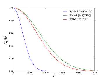
Mission	$\theta_{\rm FWHM}$	$\sigma_{\rm pix}$	$\Omega_{\rm pix}$	Frequency
Planck	7.1’	$2.2\times 10^{-6}$	0.0349	143 (GHz)
EPIC	5.0’	$8\times 10^{-9}$	0.002	150 (GHz)

Table 1: Parameters used to calculate the simulated noise and beam transfer functions for the Planck and EPIC experiment :2006uk ; Baumann:2008aq . We obtained WMAP noise and beam function from publicly available data.

Figure 5: Noise and $b_{l}$ relation, $N_{l}/b_{l}^{2}$, for each experiment plotted against $C_{l}$ taken from WMAP 7-Year best fit parameters. The frequency band used for each experiment is in brackets.

Working in spherical harmonic space, it is easy to correct our estimators ${{\cal K}}_{l}^{(2,2)}$ and ${{\cal K}}_{l}^{(3,1)}$ for the effects due to noise and the beam. All that must be done is to preform the transformation:

$$C_{L}\rightarrow C_{l}+{N_{l}\over b_{l}^{2}}.$$ (99)

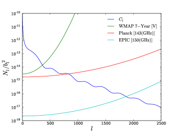
in the denominator of Eq. 89 and 89. As should be intuitively expected, a large amount of noise, or poor resolution will result in a smaller signal-to-noise. Therefore, how much the signal-to-noise is effected is related to the relationship between $C_{l}$ and $N_{l}/b_{l}^{2}$. For $N_{l}/b_{l}^{2}>>C_{l}$, the signal is greatly diminished. The relation between $C_{l}$ and $N_{l}/b_{l}^{2}$ for the WMAP, Planck and EPIC experiments is plotted in Figure 5

IV.3 Mask And Cut Sky

To remove cut sky effects using the traditional $S_{3}$ estimator, many linear terms must be computed that must be subtracted off Creminelli:2005hu ; Yadav:2007ny ; Komatsu:2008hk . Furthermore, the number of terms that must be computed grows for higher n-correlation functions. The difficulty arises because the cut sky effects are compressed into a single number, making it difficult to subtract out.

One advantage of probing primordial non-Gaussianity with skewness power spectra is that we can use techniques pioneered by Hivon et al. to remove mask effects from the spectra Hivon:2001jp . This technique is relatively simple and works identically for correlation functions of arbitrary order.

When one uses realistic data, a mask $W({\bf n})$ must be applied to an all sky map $M({\bf n})$ to get rid of unwanted sources such as the galactic plane. This mask therefore affects the $a_{lm}$s derived from the all sky $A(r,{\bf{\hat{n}}})$ and $B(r,{\bf{\hat{n}}})$ defined in equations 55 and 56 used in the bispectrum and trispectrum analysis producing cut sky $\tilde{a}_{lm}$s:

$$\tilde{a}_{lm} = \int d{{\bf{\hat{n}}}}M({\bf{\hat{n}}})W({\bf n})Y^{m*}_{l}({\bf{\hat{n}}}),$$ (100)

$$= \sum_{l^{\prime}m^{\prime}}a_{l^{\prime}m^{\prime}}\int d{{\bf{\hat{n}}}}Y^{m^{\prime}}_{l^{\prime}}({{\bf{\hat{n}}}})W({\bf{\hat{n}}})Y^{m*}_{l}({{\bf{\hat{n}}}}),$$ (101)

$$= \sum_{l^{\prime}m^{\prime}}a_{l^{\prime}m^{\prime}}K_{lml^{\prime}m^{\prime}}[W],$$ (102)

Here $a_{l^{\prime}m^{\prime}}$ is for the full sky, $M({\bf{\hat{n}}})$ represents an arbitrary full sky map and $K_{\ell ml^{\prime}m^{\prime}}[W]$ now contains all the cut sky information.

Hivon et al. showed that a power spectrum based on such masked data can be corrected by:

$$\tilde{C}_{l}=\sum_{l^{\prime}}M_{ll^{\prime}}C_{l^{\prime}},$$ (103)

where $M_{ll^{\prime}}$ is a matrix defined by

$$M_{ll^{\prime}}=\frac{2l^{\prime}+1}{4\pi}\sum_{l^{\prime\prime}}(2l^{\prime\prime}+1){W}_{l^{\prime\prime}}{\left(\begin{array}[]{lcr}l&l^{\prime}&l^{\prime\prime}\\ 0&0&0\end{array}\right)}^{2}.$$ (104)

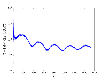
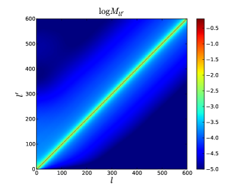
Here ${W}_{l}$ is the power spectrum of the mask $W({\bf n})$. The power spectrum for the KQ75 mask is plotted in Figure 6 and the corresponding $M_{ll^{\prime}}$ is plotted in Figure 7.

Figure 6: The power spectrum $W_{l}$ of the KQ75 mask.

Figure 7: The matrix $M_{ll^{\prime}}$ used for correcting the cut sky taken from the KQ75 mask.

Furthermore, it has been shown that any power spectra of rank $C_{l}^{(p,q)}$ for any $p$ and $q$ can be corrected with the same method using $M_{ll^{\prime}}$ Munshi:2009wy . Thus, we can correct the skewness and kurtosis power spectrum estimators for the bispectrum (rank $p$ = 2, $q$ = 1) and the trispectrum (rank $p$ = 2, $q$ = 2 and rank $p$ = 3, $q$ = 1) using this same technique. For example, a plot showing the effectiveness of this correction on the $K_{l}^{(2,2)}$ estimator is seen in figure 8.

Figure 8: On the bottom we see the results of 250 full sky gaussian simulations of ${\cal K}_{l}^{(2,2)}$ with the cut sky results without correcting with $M_{ll^{\prime}}$. On the top we see the same except the cut sky has received the proper correction.

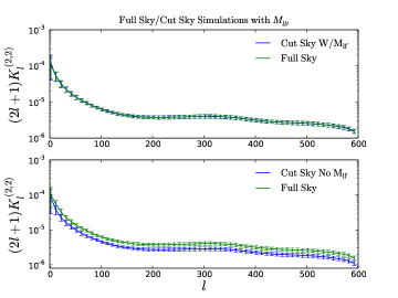
This correction technique is unique to the power spectrum approach to detect non-Gaussianity because not all $l$ dependent effects of the mask have collapsed into a single number. Therefore, the ability to correct for the mask in this approach is much easier and more efficient than calculating linear terms needed to correct for masking effects in for the traditional skewness statistic $S_{3}$.

V Fisher Analysis and Results

We now calculate the signal-to-noise for each of our estimators in order to give reasonable expectations for non-Gaussianity detection from upcoming experiments using skewness and kurtosis power spectra. These constraints assume only temperature data from one frequency band per experiment is used. For the WMAP 7-Year analysis we use the V frequency band and for Planck and EPIC we use the 143 and 150 GHz frequency bands respectively. The noise and beam for the WMAP 7-Year V band was taken from the WMAP team and those for Planck and EPIC were computed using the values in Table 1 as described in Section IV.2 .

It should be noted that combining different frequency bands and adding polarization can further reduce the expected error. For example. with the recent WMAP 7-year findings error bars on $f_{\rm NL}$ from one frequency band, V or W, is $\pm 24$ but the full temperature analysis combining V+W bands gives a reduced error bar of $\pm 21$. (About a 12.5% improvement over one temperature frequency band alone.)

For each of these calculations $C_{l}$, $\alpha(r)$, $\beta(r)$ and $F_{L}(r_{1},r_{2})$ were calculated from Eq. III.1 and  81 using a modified version of CAMB based on the WMAP 7-Year best fit cosmological parameter values. The quantities $C_{l}$, $\alpha(r)$ and $\beta(r)$ are plotted in Figure 3.

For the bispectrum we can form one skewness power spectrum estimator $C_{l}^{(2,1)}$ which places bounds on the first order non-Gaussian parameter $f_{\rm NL}$. To calculate the signal-to-noise, we compute Eq. 91 from Eq. 64 summing all $l$ up to some $l_{\rm max}$ between $2<l<1000$. After calculating this signal-to-noise we calculate the $l_{\rm max}$ dependent error bars from the Fisher matrix in eq. 94.

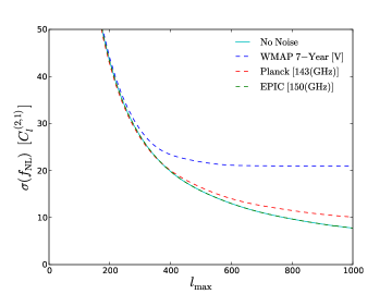
The results of this calculation are seen in Fig.9 and shown in Table 2. This calculation is done for the case of no noise nor beam, as well as with the noise and beam for the experiments WMAP 7-Year, Planck and EPIC. As, expected, the error bars drop for higher $l_{\rm max}$ until one reaches the limits of detection for each experiment. For the case with no noise, the error bars fall off as $\sim 1/\sqrt{f_{\rm NL}l^{2}}$.

Figure 9: Fisher bounds on $f_{\rm NL}$ for the ${\cal C}_{l}^{(2,1)}$ estimator of the bispectrum. This is calculated from a model with $f_{\rm NL}=1$. The frequency band used for each experiment is in brackets.

For the trispectrum we can form two skewness power spectrum estimators, ${\cal K}_{l}^{(2,2)}$ and ${\cal K}_{l}^{(3,1)}$. For primordial non-Gaussianity detection that together place bounds on the second order non-Gaussian parameters $\tau_{\rm NL}$ and $g_{\rm NL}$. The first of these, ${\cal K}_{l}^{(2,2)}$, is computed from eq. 89. After this calculation, the signal-to-noise is computed from eq. 92 summing all $l$ up to some $l_{\rm max}$ between $2<l<1000$ for all $l$ except the diagonal one. (The diagonal being the $l$ in parenthesis of $T^{l_{1}l_{2}}_{l_{3}l_{4}}(l)$.) It was confirmed, as was previously reported Kogo:2006kh , that nearly all the signal-to-noise can be calculated only summing up the $l$ in the diagonal of the trispectrum up to $l=10$, saving a tremendous amount of computational time. In this analysis, however, we summed up the diagonal in both trispectrum estimators to $l=20$ so as to be more conservative. The error bars on $\tau_{\rm NL}$ and $g_{\rm NL}$ from this estimator are then computed from equation eq. 94.

Figure 10: On top we have Fisher bounds on $\tau_{\rm NL}$ for the ${\cal K}_{l}^{(2,2)}$ estimator and on bottom for ${\cal K}_{l}^{(3,1)}$. The frequency band used for each experiment is in brackets.

Figure 11: Top: Fisher bounds on $g_{\rm NL}$ for the ${\cal K}_{l}^{(2,2)}$ estimator. Bottom: Fisher bounds on $g_{\rm NL}$ for the ${\cal K}_{l}^{(3,1)}$ estimator. The frequency band used for each experiment is in brackets.

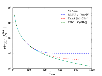
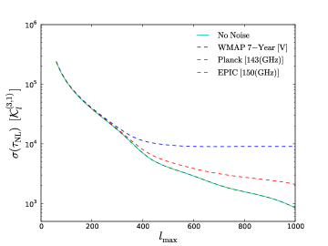
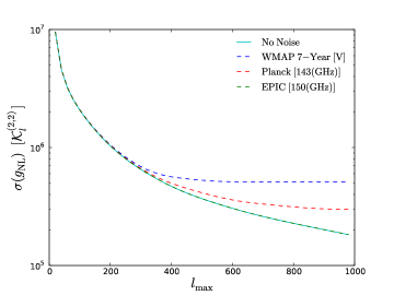
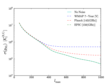
Results from this estimator for $\tau_{\rm NL}$ are seen in Fig. 10. As with the $C_{l}^{(2,1)}$ estimator above, we show the 1$\sigma$ bound for the case without noise and beam as well as for the WMAP 7-Year, Planck and EPIC experiments. For the case of no noise or beam, the error bars for this estimator fall off as $\sim 1/\sqrt{\tau_{\rm NL}l^{4}}$.

Also plotted in the figure is the amplitude $A_{\rm NL}$ assuming $f_{\rm NL}=32$, the WMAP 7-year best fit value. Therefore, if $f_{\rm NL}=32$ than we must have $A_{\rm NL}>1$ for Planck to be able to have a detection of $\tau_{\rm NL}$. However, even if $A_{\rm NL}\sim 1$, EPIC should be able to detect $\tau_{\rm NL}$, especially since EPIC will be able to use data much past $l_{\rm max}=1000$.

We also compute error bars for $\tau_{\rm NL}$ from our second skewness power spectrum estimator for the trispectrum ${\cal K}_{l}^{(3,1)}$ by first calculating the signal-to-noise from Eq. 90 and 93 then solving for $\sigma(\tau_{\rm NL})$ from the fisher matrix 94. Results for this calculation are plotted in Fig. 10. Along with the 1$\sigma$ error bars for each experiment, is the amplitude $A_{\rm NL}$ assuming $f_{\rm NL}=50$. The purpose of setting the amplitude to this value is to demonstrate that if $f_{\rm NL}$ is large enough, models with $A_{\rm NL}<1$ may be able to be tested by upcoming experiments, especially EPIC.

In addition to $\tau_{\rm Nl}$, bounds can be put on $g_{\rm NL}$ from the two before mentioned four point estimators. To do this, we calculate the estimators from eq. 89 and 90 setting $\tau_{\rm NL}=0$ and $g_{\rm NL}=1$. From here, we calculate the signal-to-noise from eq. 92 and 93 whereupon we compute Fisher bounds from equation 94. The results are seen in Fig. 11.

Combining the two estimators ${\cal K}_{l}^{(2,2)}$ and ${\cal K}_{l}^{(3,1)}$ gives the minimum error bars for $\tau_{\rm NL}$ and $g_{\rm NL}$ seen in Table 2 as well as Figure 12. These are comparable to those of Kogo:2006kh and Okamoto:2002ik who calculated Fisher bounds assuming only cosmic variance limited sky. They did not use the power skewness estimator, however, their estimator is equivalent in the limit of homogeneous noise Komatsu:2010fb . Kogo and Komastu Kogo:2006kh found a higher signal-to-noise than did Okamoto and Hu Okamoto:2002ik . This paper finds a signal-to-nose in between these values.

$l_{\rm max}$	500	1000	1500	2000
$f_{\rm NL}$ Planck	16	10	8	8
EPIC	15	7.5	5	3
$\tau_{\rm NL}$ Planck	4350	1640	1550	1550
EPIC	3700	920	400	225
$g_{\rm NL}$ Planck	$1.6\times 10^{5}$	$1.4\times 10^{5}$	$1.3\times 10^{5}$	$1.3\times 10^{5}$
EPIC	$1.5\times 10^{5}$	$1.1\times 10^{5}$	$8.4\times 10^{4}$	$6.0\times 10^{4}$
$A_{\rm NL}$ Planck	$3.0$	$1.1$	$1.0$	$1.0$
EPIC	$2.5$	$0.6$	$0.3$	0.15

Table 2: The minimum error bars at 1$\sigma$ for $f_{\rm NL}$, $\tau_{\rm NL}$ and $g_{\rm NL}$, using both ${\cal K}_{l}^{(2,2)}$ and ${\cal K}_{l}^{(3,1)}$ estimators, for the Planck and EPIC experiments up to $l_{\rm max}=2000$. As stated in text, this assumes only one temperature frequency band is used in the analysis.

Figure 12: Fisher confidence intervals for $f_{\rm NL}$, $g_{\rm NL}$ and $\tau_{\rm NL}$. The dark and light blue represent the 68% and 95% intervals respectively for Planck. The red and orange represent the 68% and 95% intervals respectively for EPIC.

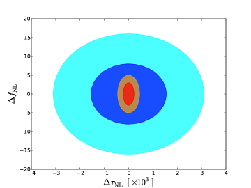
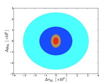
From this table we see that $\tau_{\rm NL}$ can be detected at $95\%$ confidence level by Planck if $\tau_{\rm NL}>3000$ and EPIC for $\tau_{\rm NL}>600$. If $f_{\rm NL}=32$ in the bispectrum, this equivalently means $\tau_{\rm NL}$ can be detected if $A_{\rm NL}>2$ and $A_{\rm NL}>0.4$ respectively, again alluding to the fact that EPIC will be able to test some inflationary models with $A_{\rm NL}<1$.

Furthermore, as can be seen in Fig. 13, for large enough $A_{\rm NL}$, the trispectrum is more sensitive to non-Gaussianity, even for Planck. This may turn out to be very important as some models predict $A_{\rm NL}>1$. It is therefore imperative that Planck examines the trispectrum for non-Gaussianity as it may turn out to be more likely to get a detection there than in the bispectrum.

Figure 13: Comparison of the sensitivity of both the bispectrum and the trispectrum to non-Gaussianity assuming different values of $f_{\rm NL}$ and $A_{\rm NL}$.

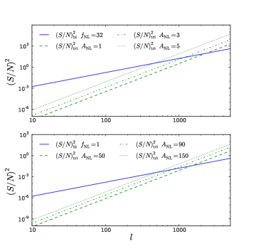
Some models predict an undetectable amount of non-Gaussianity in the bispectrum (For example, $f_{\rm NL}\sim 1$) with a large amount of non-Gaussianity in the trispectrum. These plots let us know just how big $A_{\rm NL}$ must be in order for a detection of non-Gaussianity to be made in the trispectrum for such scenarios.

From these plots we see, for $f_{\rm NL}=1$, the trispectrum becomes more sensitive to non-Gaussianity than the bispectrum at $l=1450$, $830$, and $500$ for $A_{\rm NL}=50$, 90 and 120 respectively. For $f_{\rm NL}=32$, the trispectrum has more sensitivity at $l=2350$, $1150$, and $450$ for $A_{\rm NL}=1$, 3 and 10 respectively and for $f_{\rm NL}=50$ we have more sensitivity at $l=1500$, $750$, and $300$ for $A_{\rm NL}=1$, 3 and 10 respectively.

Figure 14 shows $(A_{\rm NL}-1)/\Delta A_{\rm NL}$ for both Planck and EPIC. In this plot it is clear that both Planck and EPIC are in a position to rule out single field inflation by determining $A_{\rm NL}\neq 1$. Large sections of the parameter space, consistent with current measurements, will rule out $A_{\rm NL}$ equal to unity by $>5\sigma$.

Figure 14: The top plot shows $(A_{\rm NL}-1)/\Delta A_{\rm NL}$ for Planck and the bottom for EPIC. The color bands show to how many sigma $A_{\rm NL}$ would differ from unity for possible best fit values for Planck and EPIC. If Planck or EPIC find best fit $f_{\rm NL}$ and $\tau_{\rm NL}$ values anywhere in the white region, single-field inflation will be ruled out by $>5\sigma$. The black ellipse marks the 68% confidence region for the Smidt et al.(2009) best fit $f_{\rm NL}$ and Smidt et al.(2010) best fit $\tau_{\rm NL}$ values respectively Smidt:2009ir .

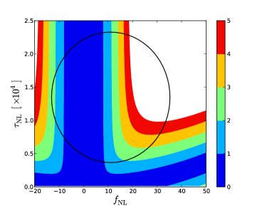
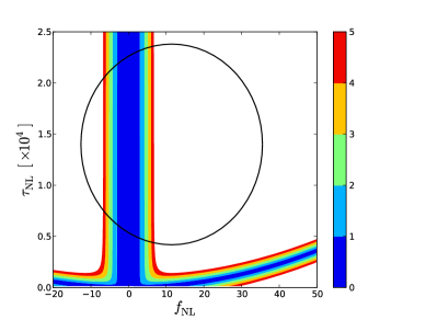
Note from table 2 that the expected bound on $g_{\rm NL}$ is about two orders of magnitude weaker than that on $\tau_{\rm NL}$, even though both parameters are suppressed by a power spectrum cubed in (21). One reason is that the $k$ dependent shape factor multiplying $\tau_{\rm NL}$ in (21) diverges whenever $k_{ij}\rightarrow 0$, while the factor multiplying $g_{\rm NL}$ only diverges when one of the $k_{i}\rightarrow 0$ (and in this case the same applies for $\tau_{\rm NL}$ as well).

VI Prior Analysis Using These Estimators

These skewness and kurtosis power spectrum estimators have recently been employed to constrain non-Gaussianity in the WMAP 5-year data. Using the bispectrum, Smidt et al. (2009) found that $-36.4<f_{\rm NL}<58.4$ at 95% confidence Smidt:2009ir . This bound puts the 1$\sigma$ error bars at $\pm 23.5$, within about 12% of the optimal Fisher bound.

The analysis for the trispectrum is more difficult and we therefore elaborate about it here. Our recipe for analysis is

1. We calculate ${\cal K}_{l}^{(3,1)}$ and ${\cal K}_{l}^{(2,2)}$ in Eq. 89- 90 for $\tau_{\rm NL}$ and $g_{\rm NL}=1$.

2. We extract ${\cal K}_{l}^{(3,1)}$ and ${\cal K}_{l}^{(2,2)}$ directly from WMAP 5-year data.

3. We perform the extraction of ${\cal K}_{l}^{(3,1)}$ and ${\cal K}_{l}^{(2,2)}$ from 250 Gaussian maps, allowing us to determine error bars and the Gaussian piece of each estimator.

4. We subtract off the Gaussian contribution to these estimators to ensure we are fitting to the non-Gaussian contribution.

5. We fit the two unknowns $\tau_{\rm NL}$ and $g_{\rm NL}$ from data using the two equations simultaneously. The amplitudes the theoretical curves must be scaled by gives the values for $\tau_{\rm NL}$ and $g_{\rm NL}$

6. We constrain $A_{\rm NL}$ by comparing $\tau_{\rm NL}$ from the trispectrum with $(6f_{\rm NL}/5)^{2}$ coming from the bispectrum.

This recipe is described in grater detail below:

First we calculate ${\cal K}_{l}^{(3,1)}$ and ${\cal K}_{l}^{(2,2)}$ theoretically using equations Eq. 78- 81 and Eq. 89- 90 for a model with $\tau_{\rm NL}$ and $g_{\rm NL}=1$. To obtain $C_{l}$ we use CAMB Lewis:1999bs with the WMAP 5-year best fit parameters and use the beam transfer functions from the WMAP team. We then obtain the connected piece using a modified version of the CMBFAST code Seljak:1996is . Plots of many of the quantities used for these calculations can be found in Ref. Smidt:2009ir .

Plots of ${\cal K}_{l}^{(2,2)}$ and ${\cal K}_{l}^{(3,1)}$ are shown in Figure 15. These curves will be compared with estimators derived from data to determine the magnitude of each statistic. Since we have two estimators, we can solve for the two unknowns $\tau_{\rm NL}$ and $g_{\rm NL}$ by fitting both estimators simultaneously.

To calculate the estimators from data, used in the lefthand side of equations (89) and (90), we use both the raw and foreground-cleaned WMAP 5-Year Stokes I maps for V- and W-bands masked with the KQ75 mask . We use the Healpix library to analyze the maps. For this analysis we only considered data out to $l_{\rm max}=600$. We correct for the KQ75 mask using a matrix $M_{ll^{\prime}}$, based on the power spectrum of the mask, as described above.

Figure 15 shows the results for ${\cal K}_{l}^{3,1}$ and ${\cal K}_{l}^{2,2}$ for the V and W frequency bands extracted from the raw WMAP 5-Year maps.

Figure 15: The top plot shows the ${\cal K}_{l}^{3,1}$ and ${\cal K}_{l}^{2,2}$ estimators, shown in green and blue respectively, taken from data for the W band. The same estimators for the V band are shown on the bottom. Additionally on the top the theoretical contributions for ${\cal K}_{l}^{2,2}$ and ${\cal K}_{l}^{3,1}$ proportional to $\tau_{\rm NL}$ are shown with the bottom showing those proportional to $g_{\rm NL}$. The Gaussian contributions were not removed from these plots.

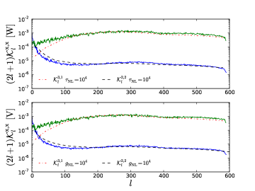
In order to do proper statistics for our data fitting we create 250 simulated Gaussian maps of each frequency band with $n_{\rm side}=512$. To obtain Gaussian maps we run the synfast routine of Healpix with an in-file representing the WMAP 5-year best-fit CMB anisotropy power spectrum and generate maps with information out to $l=600$. We then use anafast, without employing an iteration scheme, masking with the $KQ75$ mask, to produce $a_{lm}$’s for the Gaussian maps out to $l=600$. Obtaining estimators from these Gaussian maps allows us to uncover the Gaussian contribution to each estimator in addition to providing us information needed to calculate the error bars on our results.

This whole process is computationally intensive. To calculate all theoretical estimators took nearly 8,000 CPU hours. Furthermore, all the estimators from Gaussian and data maps combined took an additional 1600 CPU hours.

Figure 16: The relation between the full estimators coming from data versus the Gaussian contributions. The green curve show the Gaussian contributions coming from averaging the estimators from the Gaussian maps. The red curve is the theoretical Gaussian piece calculated using the WMAP-5 best-fit cosmology power spectrum. The error bars show two standard deviations from the Gaussian curves. These curves are from W band data.

Figure 17: The 95% confidence levels for $g_{\rm NL}$ versus $\tau_{\rm NL}$. The red and orange represent the 68% and 95% intervals respectively for the combined V+W analysis. The light blue regions represent the 95% confidence intervals for the V band analysis, and the light green regions are for the W band.

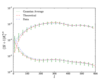
As previously discussed, the full trispectrum can be decomposed into both a Gaussian and non-Gaussian or connected piece. To make a measurement of non-Gaussianity we to subtract off the Gaussian piece from the full trispectrum. Figure 16 shows the the relationship between the full trispectrum and the Gaussian piece. In this plot the Gaussian piece was calculated in two different ways as a sanity check. First, the Gaussian maps were averaged over. Second, the Gaussian piece of each estimator is calculated theoretically using Eq. III.2.

Band	W	V	V+W
Raw
$g_{\rm NL}$	$4.7\times 10^{4}\pm 5.3\times 10^{5}$	$4.6{\rm x}10^{4}\pm 5.9\times 10^{5}$	$4.7{\rm x}10^{4}\pm 3.9\times 10^{5}$
$\tau_{\rm NL}$	${(1.63\pm 1.27)}\times 10^{4}$	${(1.68\pm 1.31)}\times 10^{4}$	${(1.64\pm 0.98)}\times 10^{4}$
$A_{\rm NL}$	$7.4\pm 7.3$	$6.3\pm 6.0$	$11.1\pm 7.3$
FC
$g_{\rm NL}$	$4.2\times 10^{4}\pm 5.3\times 10^{5}$	$4.1\times 10^{4}\pm 5.9\times 10^{5}$	$4.2\times 10^{4}\pm 3.9\times 10^{5}$
$\tau_{\rm NL}$	${(1.32\pm 1.27)}\times 10^{4}$	${(1.39\pm 1.31)}\times 10^{4}$	${(1.35\pm 0.98)}\times 10^{4}$
$A_{\rm NL}$	$6.0\pm 6.7$	$5.2\pm 5.7$	$9.2\pm 6.1$

Table 3: Results for each frequency band to $1\sigma$. Values for $g_{\rm NL}$, $\tau_{\rm NL}$ and $A_{\rm NL}$ on the top are for raw maps. The values on the bottom are for foreground clean maps. $A_{\rm NL}$ is estimated assuming $f_{\rm NL}=32\pm 21$ from the WMAP-7 analysis and the tabulated 1$\sigma$ uncertainy is based on an analytical error propagation.

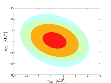
After obtaining the theory, data and simulated curves we use the best fitting procedure described in Smidt:2009ir where we minimize $\chi^{2}$ to fit $\tau_{\rm NL}$ and $g_{\rm NL}$ simultaneously. Our results are listed in Table 3. We see that $g_{\rm NL}$ and $\tau_{\rm NL}$ are consistent with zero with 95% confidence level ranges $-7.4<g_{\rm NL}/10^{5}<8.2$ and $-0.6<\tau_{\rm NL}/10^{4}<3.3$ for V+W-band in foreground-cleaned maps. The 95% confidence intervals of $g_{\rm NL}$ versus $\tau_{\rm NL}$ are plotted in Figure 17 for each band. For a V band analysis alone, the 68% confidence intervals are $\tau_{\rm NL}=(1.39\pm 1.31)\times 10^{4}$ and $g_{\rm NL}=4.6\times 10^{4}\pm 5.9\times 10^{5}$. These error bars are within $\sim$40% and $\sim$20% of the optimal Fisher values discussed above comparing with WMAP 7-year level noise for $\tau_{\rm NL}$ and $g_{\rm NL}$ respectively.

Combining $f_{\rm NL}=11\pm 24$ from Ref. Smidt:2009ir and $\tau_{\rm NL}=(1.35\pm 0.98)\times 10^{4}$ from our skewness analysis we get $-649<A_{\rm NL}<805$ at 95% confidence. If instead we had assumed $f_{\rm NL}=32\pm 21$ from WMAP-7 analysis Komatsu:2010fb and same $\tau_{\rm NL}$ reported here we find $-3<A_{\rm NL}<21.4$ at 95% confidence. The difference of the two estimates is a reflection on the central value of $f_{\rm NL}$ since $A_{\rm NL}$ = $\tau_{\rm NL}/(6f_{\rm NL}/5)^{2}$ and therefore a smaller $f_{\rm NL}$ results in a larger uncertainty in $A_{\rm NL}$. This behavior is also seen in Fig. 14.

No measurements involving WMAP 7-year data have been preformed using these estimators. It is our opinion that the results for WMAP 7-year data will not be much different than for the WMAP 5-year data, just as the optimal results using the traditional skewness statistic $S_{3}$ do not differ significantly between these two data sets. Smith:2009jr ; Komatsu:2010fb

Planck, on the other hand, is in a position to make significant improvements in the measurement of non-Gaussianity using these estimators. Since Planck is taking data, we encourage any plans to measure $f_{\rm NL}$, $g_{\rm NL}$ and $\tau_{\rm NL}$ using the skewness and kurtosis spectrum statistics that we have proposed. In addition to ruling out the standard single-field slow-roll inflation model with a detection of non-Gaussianity in general, Planck is in a position to possibly rule out all single-field models with a measurement of $A_{\rm NL}\neq 1$.

VII Conclusions

In this paper we discussed the skewness and kurtosis power spectrum approach to probing primordial non-Gaussianity. We outlined the expected constraints these techniques will place using future experimental data. These constraints were calculated by computing the signal-to-noise for each estimator, properly taking into account the noise and beam of each experiment. Optimal error bars for $f_{\rm NL}$, $g_{\rm NL}$ and $\tau_{\rm NL}$ are listed as a function of $l_{\rm max}$.

It was argued that the skewness and kurtosis power spectrum approach to measure non-Gaussianity has several advantages. These advantages include the ability to separate foregrounds and other secondary non-Gaussian signals, the ability to measure the scale dependance of each statistic and an advantage that the cut sky can be corrected from a matrix $M_{ll^{\prime}}$ without needing to compute extra linear terms.

The physical significance of each non-Gaussian statistic is discussed. In the bispectrum, different non-Gaussian triangle configurations in Fourier space contributing to $f_{\rm NL}$ are related to different underlying physics. By adding a local measurement of the trispectrum, a new statistic $A_{\rm NL}=\tau_{\rm NL}/(6f_{\rm NL}/5)^{2}$ will be a powerful probe to distinguish between multi-field models. Single-field models can be ruled out in general if $A_{\rm NL}\neq 1$ and we discussed how this may be a real possibility with Planck or EPIC. Furthermore, for $A_{\rm NL}$ large enough, the trispectrum becomes a better probe for non-Gaussinity than the bispectrum for analysis utilizing information on very small scales. The parameter $g_{\rm NL}$ will be the hardest to constrain. A constraint on this parameter will uncover information on self-interactions.