Modeling the Time Variability of SDSS Stripe 82 Quasars as a Damped Random Walk

Abstract

We model the time variability of $\sim$9,000 spectroscopically confirmed quasars in SDSS Stripe 82 as a damped random walk. Using 2.7 million photometric measurements collected over 10 years, we confirm the results of Kelly et al. (2009) and Kozłowski et al. (2010) that this model can explain quasar light curves at an impressive fidelity level (0.01-0.02 mag). The damped random walk model provides a simple, fast [O($N$) for $N$ data points], and powerful statistical description of quasar light curves by a characteristic time scale ($\tau$) and an asymptotic rms variability on long time scales ($SF_{\infty}$). We searched for correlations between these two variability parameters and physical parameters such as luminosity and black hole mass, and rest-frame wavelength. Our analysis shows $SF_{\infty}$ to increase with decreasing luminosity and rest-frame wavelength as observed previously, and without a correlation with redshift. We find a correlation between $SF_{\infty}$ and black hole mass with a power law index of 0.18$\pm$0.03, independent of the anti-correlation with luminosity. We find that $\tau$ increases with increasing wavelength with a power law index of 0.17, remains nearly constant with redshift and luminosity, and increases with increasing black hole mass with power law index of 0.21$\pm$0.07. The amplitude of variability is anti-correlated with the Eddington ratio, which suggests a scenario where optical fluctuations are tied to variations in the accretion rate. However, we find an additional dependence on luminosity and/or black hole mass that cannot be explained by the trend with Eddington ratio. The radio-loudest quasars have systematically larger variability amplitudes by about 30%, when corrected for the other observed trends, while the distribution of their characteristic time scale is indistinguishable from that of the full sample. We do not detect any statistically robust differences in the characteristic time scale and variability amplitude between the full sample and the small subsample of quasars detected by ROSAT. Our results provide a simple quantitative framework for generating mock quasar light curves, such as currently used in LSST image simulations.

1 Introduction

The optical variability of quasars has been recognized since they were first identified (Matthews & Sandage 1963). Indeed, most quasars are variable ($\sim$90% at the 0.03 mag rms level; Sesar et al. 2007), and the variations in brightness are aperiodic and on the order of 20% on time scales of months to years (e.g., Hook et al. 1994; Vanden Berk et al. 2004). Furthermore, the smooth power spectra suggest a chaotic, or stochastic, origin for the variability. A range of models have been advanced to describe quasar variability, including supernova bursts, microlensing, and accretion disk instabilities (Aretxaga et al. 1997; Hawkins 1993; Kawaguchi et al. 1998; Trèvese & Vagnetti 2002). These models are discussed and compared in Hawkins (2007). Reverberation mapping studies (e.g., Peterson et al. 2005) show that the broad emission lines respond to continuum fluctuations, therefore providing strong evidence that the variability is intrinsic to the quasars. A number of studies have utilized standard accretion disk models to demonstrate that the optical-UV variability of quasars could be driven by a variable accretion rate (e.g., Pereyra et al. 2006; Li & Cao 2008; Liu et al. 2008). Blackburne & Kochanek (2010) find evidence in the light curves of microlensed quasars that the optical variability is caused by a change in the effective area of the accretion disk.

Recently, Kelly et al. (2009, hereafter KBS09) proposed a model where the optical variability is described by a damped random walk (a self-correcting term added to a random walk model that acts to push any deviations back towards the mean value). They proposed that the variability time scale might be identified with the thermal time scale of accretion disks, as also proposed by Collier & Peterson (2001). A thermal origin of the variability would explain why quasars become bluer as they brighten (e.g., Giveon et al. 1999; Trèvese et al. 2001; Geha et al. 2003).

Although the physical causes have yet to be proven, it has been established by KBS09 and Kozłowski et al. (2010a, hereafter Koz10) that a damped random walk can statistically explain the observed light curves of quasars. Using 100 well-sampled single-band light curves compiled from the literature, KBS09 show that this stochastic process is capable of modeling complex quasar light curves at an impressive fidelity level (0.01-0.02 mag). Koz10 applied the model to the OGLE light curves (Udalski et al. 1997; Udalski et al. 2008) of mid-infrared-selected quasars behind the Magellanic Clouds from Kozłowski & Kochanek (2009). Their analysis shows that this stochastic model is robust enough to efficiently select quasars from other variable sources (see Schmidt et al. 2010 for a different method of selecting quasars based on variability). The model has only three free parameters: the mean value of the light curve, the driving amplitude of the stochastic process, and the damping time scale. The predictions are only statistical, and the random nature reflects our uncertainty about the details of the physical processes.

Instead of applying a model to observed light curves for individual quasars, numerous studies have looked at the ensemble variability of quasars, particularly in samples where individual light curves are not available. Significant progress in the description of quasar variability has been made by employing the Sloan Digital Sky Survey (SDSS) data (Vanden Berk et al. 2004, hereafter VB04; Ivezić et al. 2004, hereafter I04; de Vries et al. 2005; Wilhite et al. 2005, 2006, 2008; Sesar et al. 2006). For example, the size and quality of the sample analyzed by VB04 (two-epoch photometry for 25,000 spectroscopically confirmed quasars) allowed them to constrain how quasar variability in the rest frame optical/UV regime depends upon rest-frame time lag (up to $\sim$2 years), luminosity, rest wavelength, redshift, the presence of radio and X-ray emission, and the presence of broad absorption line systems. Using repeated SDSS photometric observations, Wilhite et al. (2008) confirmed the result of Wold et al. (2007) that variability is correlated with black hole mass, and show that this is independent of the anti-correlation between variability and luminosity established by many studies. This led them to suggest that the amplitude of variability may be driven by the quasar’s Eddington ratio, implying differences in accretion rate.

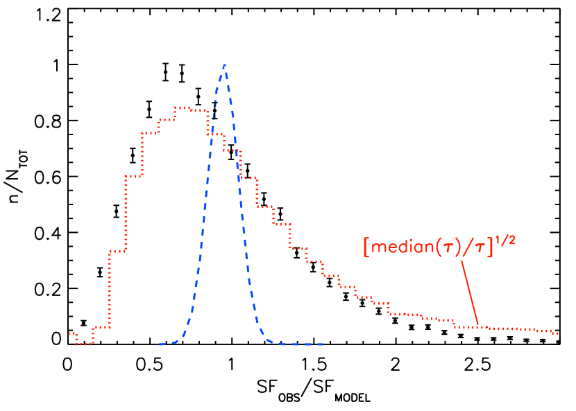
These studies typically quantify the observed optical variability of quasars using a structure function (SF) analysis (see also Hughes et al. 1992; Collier & Peterson 2001; Bauer et al. 2009; Kozłowski et al. 2010b), where the SF is the root-mean-square (rms) magnitude difference as a function of the time lag ($\Delta t$) between measurements. This autocorrelation-like function is less sensitive to aliasing and other time-sampling problems than a power spectral distribution. By studying the magnitude difference distribution for appropriately chosen subsamples with fixed values of absolute i-band magnitude ($M_{i}$), rest-frame time lag ($\Delta t_{RF}$, in days), and wavelength ($\lambda_{RF}$, in Å), the mean dependence of the SF on these quantities was inferred by I04 to be

$$SF_{model}=A[1+B\,M_{i}]\left(\frac{\Delta t_{RF}}{\lambda_{RF}}\right)^{C}\rm mag,$$ (1)

with $A=1.00\pm 0.03$, $B=0.024\pm 0.04$, and $C=0.30\pm 0.05$. A qualitatively similar result was obtained by VB04. Kozłowski et al. (2010b), in the first large study of the mid-IR structure functions of quasars, also found lower variability for higher luminosities and longer wavelengths, but the temporal slope of the ensemble structure functions were significantly steeper than in the optical. In addition, there is evidence for a turnover in the SF on long time lags (I04; Rengstorf et al. 2006; Wold et al. 2007). Studies by de Vries et al. (2005) and Sesar et al. (2006) using SDSS combined with earlier Palomar Observatory Sky Survey measurements for 40,000 SDSS quasars constrained quasar continuum variability on time scales of 10 to 50 years in the observer’s frame. They report that the characteristic time scale, which in this context is the time lag above which the SF flattens to a constant value, is of order 1 year in the quasar rest frame. Using a shot-noise light curve model, de Vries et al. (2005) found evidence for multiple variability time scales in long-term ensemble variability measurements, while Collier & Peterson (2001) found a wide range of different time scales in their analysis of individual light curves, and even evidence for multiple time scales in a single active galactic nucleus (AGN).

These analyses of ensemble variability are based on a fundamental assumption that photometric observations at two epochs for a large number of quasars will reveal the same statistical properties as well-sampled light curves for individual objects. This assumption has been tested by MacLeod et al. (2008) using light curves for spectroscopically confirmed quasars observed roughly 50 times over 8 years in SDSS Stripe 82 (S82). They found that while the mean SF for individual sources is consistent with Eq. 1, the contribution of the mean trends to the observed dispersion in variability properties is minor compared to an intrinsic stochasticity of unknown origin. Further investigation of this stochastic behavior is one of the main goals of this study.

In order to better understand the relationship between the two types of data analyses (individual versus ensemble quasar variability), and to begin linking to physical models, we apply the damped random walk model to the $ugriz$ light curves of $\sim$9,000 spectroscopically confirmed SDSS S82 quasars. This large sample greatly benefits from the robust, accurate, five-band SDSS photometry. We estimate the variability parameters following Koz10, who demonstrated that their approach is more statistically powerful than the forecasting methods used by KBS09. We also note that both the Koz10 and KBS09 approaches are much faster than that used by Schmidt et al. (2010), requiring only O($N$) rather than O($N^{2}$) operations to determine the model parameters for a light curve with $N$ data points.

In Section 2, we describe the model, define our variability parameters, and demonstrate their relationship to those utilized in previous studies. In Section 3, we introduce the S82 data set and outline our initial light curve selection. In Section 4, we present the best-fit variability parameters for our final sample of light curves and estimate their scatter due to the limited time sampling of SDSS. We also estimate the sensitivity of our results to variations in the slope of the model power spectrum on long time scales. In Section 5, we describe the relationship between the long-term variability parameters and physical parameters such as wavelength, absolute magnitude, black hole mass, and Eddington ratio. Using these results, we also provide a prescription for simulating mock quasar light curves. In Section 6, we explore the variability properties of subsamples detected at radio and X-ray wavelengths. Finally, we summarize our results in Section 7.

2 Methodology

We model the time variability of quasars as a stochastic process described by the exponential covariance matrix

$$S_{ij}=\sigma^{2}\exp(-|t_{i}-t_{j}|/\tau)$$ (2)

between times $t_{i}$ and $t_{j}$. As detailed by KBS09 and Koz10, this corresponds to a damped random walk (more specifically, an Ornstein-Uhlenbeck process) with a damping time scale $\tau$, also called the characteristic time scale, and a long-term standard deviation of variability $\sigma$. Following Koz10, we model the light curves and estimate the parameters and their uncertainties using the method of Press et al. (1992), its generalization in Rybicki & Press (1992), and the fast computational implementation described in Rybicki & Press (1994). Koz10 demonstrate that this approach is more statistically powerful than the forecasting methods used by KBS09, while still having computation times scaling linearly with the number of data points.

2.1 Structure Function for the Damped Random Walk Model

For our analysis, we express the long-term variability in terms of the structure function (SF) in order to relate to our previous studies and to those of two-epoch samples. The first order SF is $SF^{2}(\Delta t)=2\sigma^{2}[1-ACF(\Delta t)]$ (e.g., Hughes et al. 1992), where the autocorrelation function for a damped random walk is $ACF(\Delta t)=\exp{(-|\Delta t|/\tau)}$ (Eq. A6 in KBS09). This ACF results in the structure function:

$$SF(\Delta t)=SF_{\infty}(1-e^{-|\Delta t|/\tau})^{1/2}.$$ (3)

Asymptotic values of the SF at large and small $\Delta t$ are

$$SF(\Delta t>>\tau)\equiv SF_{\infty}=\sqrt{2}\sigma$$

$$SF(\Delta t<<\tau)=\sigma\sqrt{\frac{2|\Delta t|}{\tau}}=SF_{\infty}\sqrt{\frac{|\Delta t|}{\tau}}$$ (4)

The form $SF\propto|\Delta t|^{\beta}$ is equivalent to a power spectral distribution $PSD\propto f^{\alpha}$, where $\alpha=-2\beta-1$ (see Appendix of Bauer et al. 2009; KBS09). The SF at small time lags is therefore equivalent to a power spectral distribution $PSD\propto f^{-2}$. We adopt $SF_{\infty}$ and $\tau$ as our two main variability model parameters.

2.2 Model Light Curves

Equipped with a statistical description of quasar variability, we generate well-sampled light curves in order to 1) demonstrate the relationship between our variability parameters and the traditional SF analyses of many previous works, and 2) to estimate the systematic effects that the sampling rate and light curve length have on the fitted parameters. The latter is especially important because the S82 data are fairly sparse. As shown below and in Section 4.2, these indeed have a large impact.

A light curve is generated using only three input parameters: $SF_{\infty}$, $\tau$, and the mean value of the light curve, $\mu$. The magnitude $X(t)$ at a given timestep $\Delta t$ from a previous value $X(t-\Delta t)$ is drawn from a normal distribution with a mean and variance given by

$$E(X(t)|X(t-\Delta t))=e^{-\Delta t/\tau}X(t-\Delta t)+$$

$$\mu(1-e^{-\Delta t/\tau})$$

$$Var(X(t)|X(t-\Delta t))=0.5(SF_{\infty})^{2}(1-e^{-2\Delta t/\tau})$$ (5)

(Eqs. A4 and A5 in KBS09). The asymptotic variance of the time series is then $0.5(SF_{\infty})^{2}$. The top panel of Figure 1 shows a segment of a well-sampled light curve generated using $\tau=20$ days, $SF_{\infty}=0.14$ mag, and a time sampling of $0.1(\Delta t/\tau)$. The structure function, $SF(\Delta t)$, is computed by collecting the differences in magnitude for all points in the light curve separated by a given time lag, $\Delta t$. The distribution of magnitude differences ($\Delta m$) is Gaussian by construction, and the rms of the $\Delta m$ distribution is the $SF$ value for that time lag.

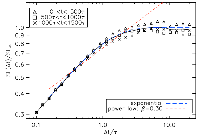
When fitting values for $SF_{\infty}$ and $\tau$ for a given light curve, the length of time that it spans plays an important role. For example, in Figure 1, the SF computed for the full light curve length of $1500\tau$ (82 years) is much smoother than that computed for three equal sections, each spanning 27 years. Therefore, the determination of variability parameters for S82 quasars will be affected by their light curve lengths, which are typically $10\tau$. When the light curve is too short, it is easy to overestimate $\tau$ because there is no information on the time scale of the break (where $SF(\Delta t)$ flattens to $SF_{\infty}$). The model will reproduce the observed variance in the light curve by overestimating $SF_{\infty}\simeq(SF_{\infty})_{true}(\tau/\Delta t)^{1/2}$, and therefore $\hat{\sigma}=SF_{\infty}/\sqrt{\tau}$ is the more robustly estimated model parameter when $\tau$ cannot be well-determined.

2.3 Comparison with Published Work

Before interpreting the form of $SF(\Delta t)$, we summarize the major differences between our S82 analysis and previous studies based on ensemble structure functions. The ensemble structure function is computed using only a few observations of many quasars, combining all magnitude differences to find $SF(\Delta t)$. Using an ensemble approach is beneficial because it enables one to constrain the average variability properties when it is difficult to constrain such quantities for individual quasars. Indeed, even with well-sampled light curves, spurious breaks in the individual SFs are common (Emmanoulopoulos, McHardy, & Uttley 2010). However, in previous works (e.g., I04; de Vries et al. 2005), the characteristic time scale is defined as the time lag at which the ensemble $SF(\Delta t)$ flattens to a constant value, and thus it represents some complex average over the intrinsic $\tau$ distribution. In contrast, by applying a stochastic model to the individual S82 light curves, we are relatively insensitive to time sampling issues (for details, see KBS09), and we obtain a model fit for every quasar in each filter described by the parameters $SF_{\infty}$ and $\tau$.

A power law fit to $SF(\Delta t)$ has previously been a common way to describe $SF(\Delta t)$, and even to reject certain classes of models (e.g., Kawaguchi et al. 1998; VB04; I04). However, Figure 1 shows that the best-fit power law index is extremely sensitive to the fitted range of $\Delta t/\tau$. For example, for $0.1<\Delta t/\tau<1$, $SF(\Delta t)$ is well fit by a power law with an index of $\sim$0.5, while for $0.15<\Delta t/\tau<3$, we obtain a strongly biased power law index of $0.3$. Furthermore, each quasar has its own values of $\tau$ and $SF_{\infty}$, and the ensemble structure function is a convolution of the individual structure functions with their distribution in parameters,

$$SF(\Delta t)=\int{\rm d}\tau{\rm d}SF_{\infty}{{\rm d}^{2}n\over{\rm d}\tau{\rm d}SF_{\infty}}SF(\Delta t|\tau,SF_{\infty}),$$ (6)

where $SF(\Delta t|\tau,SF_{\infty})$ (Eq. 3) is the structure function at time $\Delta t$ for a quasar with variability parameters $\tau$ and $SF_{\infty}$. Hence, the ensemble structure function is only indirectly related to the structure function for any particular quasar, and results based on fitting a power law to observed ensemble structure functions should be interpreted with caution.

3 The SDSS Stripe 82 Quasar Data Set

The Sloan Digital Sky Survey (SDSS, York et al. 2000) provides homogeneous and deep ($r<22.5$) photometry in five passbands ($ugriz$, Fukugita et al. 1996; Gunn et al. 1998; Smith et al. 2002) accurate to 0.02 mag, of almost 12,000 deg² in the Northern galactic cap, and a smaller, but deeper, survey of 290 deg² in the Southern galactic hemisphere. For this 290 deg² area known as Stripe 82 (S82), there are on average more than 60 available epochs of observations. These data were obtained in yearly “seasons” about 2-3 months long over the last decade, and the cadence effectively samples time scales from days to years. The light curve lengths are effectively shorter than the actual period of the survey because the better-sampled supernova observations begin about 5 years into the survey. Because some observations were obtained in non-photometric conditions, improved calibration techniques have been applied to SDSS S82 data by Ivezić et al. (2007) and Sesar et al. (2007), and we use their results. For these data, photometric zero-point errors are 0.01–0.02 mag.

We have compiled a sample of 9,275 spectroscopically confirmed quasars in S82 with re-calibrated $ugriz$ light curves (see also Bhatti et al. 2010). Most (8,974) of these are in the SDSS Data Release 5 (DR5) Quasar Catalog (Schneider et al. 2007), and the remaining are newly confirmed DR7 (Abazajian et al. 2009) quasars. Summed over all bands and epochs, the data set includes 2.7 million photometric measurements. For 41% of the sample, the random photometric errors are smaller than 0.03 mag. Only 1% have errors $\geq 0.1$ mag in $g$, $r$, and $i$, and 2.4% have errors exceeding 0.25 mag in $u$ and $z$ filters. In MacLeod et al. (2010, in prep.), these light curves, as well as a much larger sample of quasars with two SDSS epochs selected from 12,000 deg² of the sky, will be made publicly available. We adopt the K-corrected i-band absolute magnitudes from Schneider et al. (2007), and virial black hole masses and bolometric luminosities where available from Shen et al. (2008). The Shen et al. masses were estimated from emission line widths (H$\beta$ for $z<0.7$, MgII for $0.7<z<1.9$, and CIV for $z>1.9$). However, we note that at low spectroscopic signal-to-noise, black hole masses tend to be overestimated (Denney et al. 2009).

3.1 Initial Light Curve Selection

The damped random walk model was fit to all available $ugriz$ light curves for $9,275$ S82 quasars. Summed over 5 bands, there are $46,375$ best-fit values of the characteristic (damping) time scale $\tau$ and long-term structure function $SF_{\infty}$. For further analysis, we select light curves that satisfy the following criteria:

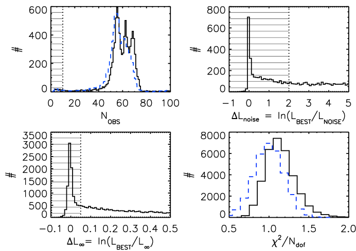
1. First, we remove light curves with fewer than 10 observations. The top-left panel of Figure 2 shows the distribution of the number of observations ($N_{obs}$) per light curve before this cut, which reduces our sample to $45,814$. At a given $N_{obs}$, the distribution of the ratio of light curve length to $\tau$ is similar to that at all other values of $N_{obs}$. Therefore, any systematic effects of $N_{obs}$ on derived parameter distributions should be small.

2. We then require that the stochastic model must provide a better fit than uncorrelated noise. Following Koz10, we select light curves with a likelihood improvement over simply broadening the measurement errors of $\Delta L_{noise}\equiv\ln{(L_{best}/L_{noise})}>2$, where $L_{best}$ is the likelihood of the stochastic model and $L_{noise}$ is that for the noise solution where $\tau\rightarrow 0$. The top-right panel of Figure 2 shows the distribution of $\Delta L_{noise}$ before this cut, which removes 14% of $u$ and $z$ light curves, whose photometric errors are larger. About 7% of our light curves (82% of which are $u$ or $z$ band) are removed in this step, reducing our total to $42,623$.

3. Finally, we remove cases where $\tau$ is merely a lower limit due to the length of the light curve. We define $\Delta L_{\infty}\equiv\ln{(L_{best}/L_{\infty})}$, where $L_{\infty}$ is the likelihood that $\tau\rightarrow\infty$, indicating that the light curve length is too short to accurately measure $\tau$. The bottom-left panel shows a peak at $\Delta L_{\infty}=0$, and we exclude these objects by requiring that $\Delta L_{\infty}>0.05$. Most (95%) of the rejected light curves have lengths $<\tau$; 76% have $\tau\geq 10^{4}$ days, and 64% have $SF_{\infty}\geq 1$ mag. The latter is due to the fact that as the $\tau$ value becomes long and uncertain, the model will necessarily overestimate $SF_{\infty}$ in order to keep the overall light curve rms fixed (see Section 2.2).

   The rejected light curves tend to be higher redshift quasars because stronger time dilation leads to shorter rest-frame light curve lengths, making it increasingly difficult to constrain long rest-frame $\tau$. This criterion removes 22% of our sample, leaving a total of $33,112$ values of $\tau$ and $SF_{\infty}$. Because we are limited by the duration of the S82 survey, this is a significant loss, and therefore our final $\tau$ distribution is biased low, but the bias should not be significant considering our results in Section 4.2.

The resulting light curves are well-fit by the stochastic model, as can be seen from the distribution of $\chi^{2}/N_{dof}$ shown in the bottom-right panel in Figure 2, where $N_{dof}$ is the number of degrees of freedom. The expected Gaussian distribution with rms $=\sqrt{2/N_{dof}}$ is also shown in the panel, where we have averaged over the $N_{dof}$ distribution of the light curves. The observed distribution is centered at $\chi^{2}/N_{dof}=1.1$. This difference is some combination of errors in the estimated errors, outliers in the light curves, and any poorly modeled physics. Koz10 noted a similar difference in their analysis of OGLE light curves. Only 5% of the light curves have $\chi^{2}/N_{dof}>1.5$, confirming that most quasars are variable (at the $\Delta L_{noise}>2$ level), and that a damped random walk is a good description of quasar variability.

4 Variability Parameters for Stripe 82 Quasars

4.1 Observed Distributions

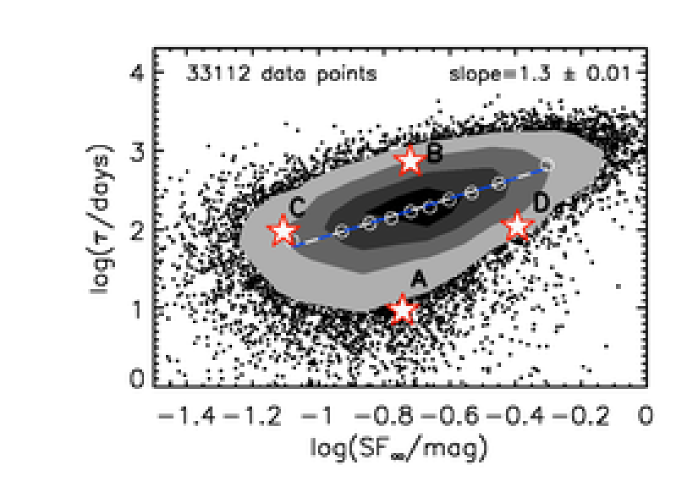
We assume the variability to be intrinsic to the quasars and convert the time scales to the rest frame (dividing by $(1+z)$) before further analysis. The long-term structure function should be independent of redshift other than through evolution in physical parameters, and this view is confirmed by KBS09. Figure 3 shows the distributions in $SF_{\infty}$ and rest-frame $\tau$ found for the S82 quasars. If we consider only the brighter ($i<19$) quasars, based on the best-fit mean magnitude, the distributions are generally similar but biased towards lower asymptotic amplitudes (peaked at 0.12 mag). The distributions are consistent with what was found in KBS09 and Koz10; however, in these studies, there are not as many objects with runaway ($\tau\rightarrow\infty$) time scales because of the improved time sampling of the OGLE survey and many of the light curves in the KBS09 sample. Also, the observed-frame $\tau$ distribution lacks many of the short time scales observed in Koz10; this is likely due to either the better time sampling of the OGLE light curves or unrecognized stellar contamination in their sample.

The bottom panel of Figure 3 shows that the best-fit variability parameters are highly correlated with each other, indicating that quasars with larger asymptotic amplitudes of variability also have longer characteristic time scales. We fit a power law slope of $1.3\pm 0.01$ dex/dex for all 33,112 data points, and this trend persists within each $ugriz$ band as well. Note that a correlation between $\tau$ and $SF_{\infty}$ is expected even if $\tau$ is independent of the driving amplitude of short-term variations, $\hat{\sigma}=SF_{\infty}/\sqrt{\tau}$. Since the power law slope of $1.3$ is steeper than that expected if $\tau$ and $\hat{\sigma}$ are independent ($\sim$0.2, see below), the time scale must also be correlated with the amplitude of short-term variability. We confirm that this correlation is intrinsic, rather than an artifact of short light curve lengths, in Section 4.2.

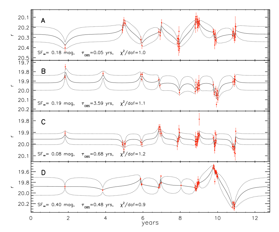
The approximate values for $\tau$ and $SF_{\infty}$ can often be guessed from light curves by simple visual inspection. Figure 4 shows representative light curves from several regions of $\tau-SF_{\infty}$ space, indicated by stars in Figure 3. The weighted average of all model light curves consistent with the data is also shown, and the “error snake” is the $\pm 1\sigma$ range of those light curves about this mean. The top panel shows a light curve with a relatively short $\tau$ – this is due to the large amount of variability within each season (i.e. each grouping of points), as compared to that in the second panel, which shows a curve with a much larger $\tau$. The third panel shows a light curve with a relatively low $SF_{\infty}$, while the bottom panel shows one with a larger $SF_{\infty}$, as can be seen by the larger difference in median $r$ band magnitude between about 10 and 11 years. Note the outlier in the third panel: outliers such as these are generally responsible for higher values of $\chi^{2}/N_{dof}$. The (data$-$model) brightness difference provides a convenient way to identify outliers, and they may be an indicator of variability behavior not captured by the damped random walk model. However, they may also be caused by occasional non-Gaussian photometric errors and thus their analysis requires a detailed and careful study (e.g., by utilizing control samples of appropriately chosen nearby non-variable stars). Since the model provides satisfactory fits for the overwhelming majority of objects (see Section 3.1), we do not further investigate such outliers in this work. We have also searched for periodic signals in observed light curves and did not find any convincing cases. This analysis is summarized in the Appendix.

4.2 The Effect of S82 Time Sampling and Estimate of Fitting Errors

There are three contributions to the scatter in the best-fit variability parameters $\tau$ and $SF_{\infty}$. First, the fitting errors, including those due to insufficient time sampling and light curve length, will introduce some scatter. Second, trends with physical parameters (see Section 5) result in a certain distribution width. There may also be scatter due to other sources of variability that are not captured by the model, such as flares, or other activity related to radio emission, for example. Here, we carry out two tests in order to understand how the best-fit parameters are affected by the limited data sampling of S82.

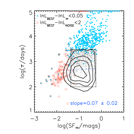
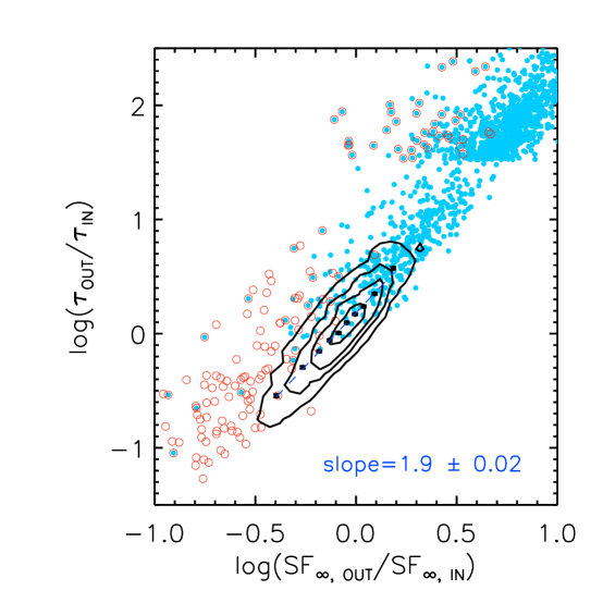
Since the correlation between $\tau$ and $SF_{\infty}$ seen in Figure 3 might be expected if the light curves are not sampled over sufficiently long periods of time (see Section 2.2), we first test whether the correlation is real or simply an artifact. We generated light curves as described in Section 2.2 using the time sampling and photometric uncertainties of the S82 data. For each object, the input parameters $\tau_{in}$ and $SF(\infty)_{in}$ are randomly drawn from a uniform distribution in $\log\tau$ and $\log SF_{\infty}$ limited by the dotted rectangle in the left panel of Figure 5. These artificial light curves are then fit to obtain $\tau_{out}$ and $SF(\infty)_{out}$, and the resulting distribution is shown by the contours in Figure 5. The open circles show data points that do not satisfy $\Delta L_{noise}>2$ (3% of all input points) – these are concentrated at small $\tau_{out}$ and $SF(\infty)_{out}$. The closed circles show those that do not satisfy $\Delta L_{\infty}>0.05$ (21% of all input points) – these have been smeared to large values of $\tau_{out}$ and $SF(\infty)_{out}$. After omitting points with $\Delta L_{noise}\leq 2$ and $\Delta L_{\infty}\leq 0.05$, the distribution of the output estimates is similar to the input distribution and shows no strong correlation between $\tau_{out}$ and $SF(\infty)_{out}$. This suggests that the correlation in Figure 3 is largely real, and not an artifact of sampling and fitting procedures. These results also justify the selection cuts outlined in Section 3.1. The right panel of Figure 5 shows the expected correlation that the larger the overestimate of $\tau$, the larger the overestimate of $SF_{\infty}$, with a slope between them following that expected by Eq. 4 (for $\Delta t<<\tau$). We repeated the test using a uniform input distribution in $\log\hat{\sigma}$ (the driving amplitude of short-term variations) rather than in $\log SF_{\infty}$, where $\hat{\sigma}=SF_{\infty}/\sqrt{\tau}$. In this case, we find the output $\tau$ and $SF_{\infty}$ are correlated with a power law slope of $0.18\pm 0.01$. Since this slope is smaller than that for the observed distribution in Figure 3, the $\hat{\sigma}$ and $\tau$ must be intrinsically correlated for the S82 sample as well.

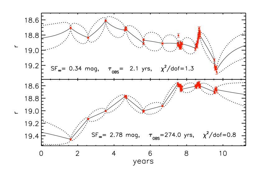
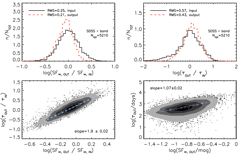
For our second test, we used the best-fit $\tau$, $SF_{\infty}$, and $\mu$ for the S82 sample to generate new light curves with the same time sampling and photometric uncertainties as the S82 data. By comparing the output and input parameter distributions, we can estimate how much the intrinsic stochasticity and the time sampling issues affect the results. Figure 6 compares an observed and “regenerated” light curve, where the differences are due to the stochastic nature of the process. The fit parameters for the “regenerated” light curve can be very different because of how the particular realization is affected by the time sampling, as illustrated in Figure 6. Figure 7 shows the ratio of output to input distributions for both $\tau$ and $SF_{\infty}$. The input distributions normalized by their median values are also shown to illustrate their dynamic range. These two distributions are compared to each other in order to estimate the effect of fitting errors (the ratio of output to input should be a delta function centered at 1 for perfect time sampling). The bottom-right panel shows that the correlation between $\tau$ and $SF_{\infty}$ becomes slightly weaker than that seen in Figure 3. Based on these results, we conclude that the uncertainties due to sparse sampling and limited lengths of the S82 light curves can account for 71% of the spread in $SF_{\infty}$ and 57% of that in $\tau$. As shown in Section 2.2, very long light curve lengths are needed to estimate accurate time scales and asymptotic amplitudes. Nevertheless, the observed distributions indicate that the underlying intrinsic distributions of $\tau$ and $SF_{\infty}$ have finite widths that are similar to the observed widths.

4.3 Relationship between the Individual SFs and the Ensemble SF

The distribution of $\tau$ is important to consider when relating the ensemble SF, such as those determined using two-epoch datasets, to the SFs for individual light curves. The analysis based on two-epoch data measures the mean value of the SF, but provides no information about the SF variance among individual objects. To measure the latter, individual light curves must be available.

MacLeod et al. (2008) analyzed individual light curves for S82 quasars in order to test the common assumption that photometric observations at two epochs for a large number of quasars will reveal the same statistical properties seen in light curves for individual objects. They found that the dependence of the mean SF computed using SFs for individual light curves on luminosity, rest-frame wavelength and time lag is indeed qualitatively and quantitatively similar to that derived from two-epoch observations of a much larger sample. However, they also found that the scatter in the light-curve based SFs for fixed values of $M_{i}$, $\lambda_{RF}$ and $\Delta t_{RF}$ is very large, and in fact, similar to the scatter for the whole sample (see Figure 8). This large scatter was attributed to an intrinsic stochasticity of unknown origin. The new model-based analysis discussed here allows us to explain this puzzling result as a consequence of the finite width of the $\tau$ distribution.

An important piece of information missing from the MacLeod et al. (2008) analysis is the existence of a characteristic time scale $\tau$. In MacLeod et al. (2008), the individual structure functions ($SF$) were computed following the standard approach with a fixed observer’s frame time lag of 1 year (and with rest-frame time lags spanning 100 to 300 days). However, Eq. 4 indicates that the SF at small time lags should be proportional to $1/\sqrt{\tau}$, indicating that the observed structure functions will vary between quasars even if they have similar $SF_{\infty}$. Indeed, the distribution of $\sqrt{\rm median(\tau)/\tau}$ has an almost identical shape and width as that of $SF/SF_{model}$ (see Figure 8). We therefore conclude that variations in $\tau$ are responsible for most of the scatter in $SF(\Delta t<<\tau)$ for quasars with similar luminosity, rest wavelength, and time lag. In addition, it is likely that the $\tau$ distribution is responsible for the exponential tails of the magnitude difference distribution for quasars reported by I04 and Sesar et al. (2006; see MacLeod et al. 2010, in prep., for further discussion). Therefore, the published structure function results based on two-epoch datasets can only be interpreted in the context of Eq. 6.

4.4 Dependence on the Underlying PSD

The analysis throughout this paper assumes that the variability is described by a damped random walk, which has a power spectral distribution (PSD) described by $PSD\propto f^{-2}$ at frequencies $f>(2\pi\tau)^{-1}$, flattening to a constant at lower frequencies. In this Section, we investigate the sensitivity of our resulting parameter distributions to the possibility that the low frequency part of the PSD is not flat. For example, the X-ray variability of Seyfert galaxies is well-described by a broken power law with a slope of $-2$ at high frequencies, breaking to a shallower slope ($-1$) at low frequencies (Arévalo et al. 2008a). Since the optical and X-ray variations are correlated (Arévalo et al. 2008b), it is plausible that the optical variability might have a similar underlying PSD. On the other hand, as reviewed by McHardy (2010), the optical and X-ray fluctuations are only correlated on time scales which are shorter than the typical characteristic optical time scale (i.e., on time scales corresponding to the $1/f^{2}$ part of the optical power spectra). If the damped random walk is a good description for the optical variability, then we might expect that the optical and X-ray fluctuations are no longer correlated on time scales longer than $\tau$, as the optical fluctuations resemble white noise on these time scales.

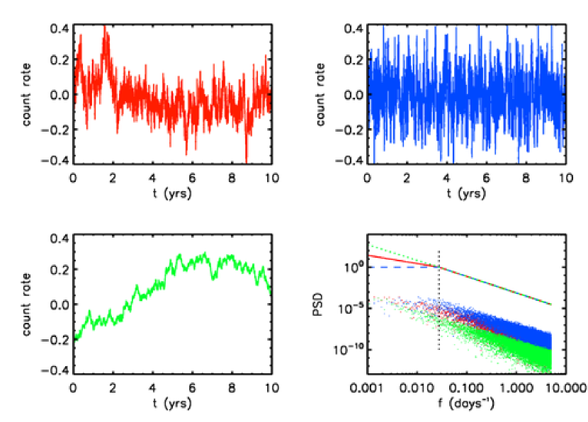
We consider three cases for a broken, or bending, PSD described by $PSD\propto f^{-2}$ at high frequencies and $PSD\propto f^{\alpha}$ at low frequencies. The first case is where $\alpha=0$, which is a damped random walk. The second case is where $\alpha=-1$, and the third is where $\alpha=-1.9$, which is nearly a constant power-law slope. In each case, $\sim$7000 light curves are simulated using the algorithm from Timmer & Koenig (1995) with the chosen PSD. For each realization, the break frequency is set to $(2\pi\tau)^{-1}$ and the total $rms$ is fixed, using the observed $r$-band $\tau$ and $rms$ values for the S82 quasars that satisfy the selection criteria in Section 3.1. Therefore, the observed distributions in Figure 3 (for the $r$-band) are the “input” values. Figure 9 shows 3 example light curves simulated using $\alpha=-1$ (red), $\alpha=0$ (blue), or $\alpha=-1.9$ (green). The lines in the last panel show each PSD from which the light curves are generated, with the black dotted line indicating the break frequency. As a check, the PSD was computed for each simulated light curve, and as seen by the colored dots, the shapes match the input.

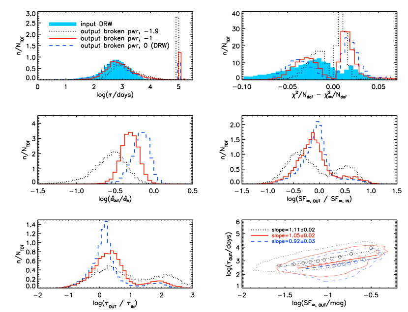
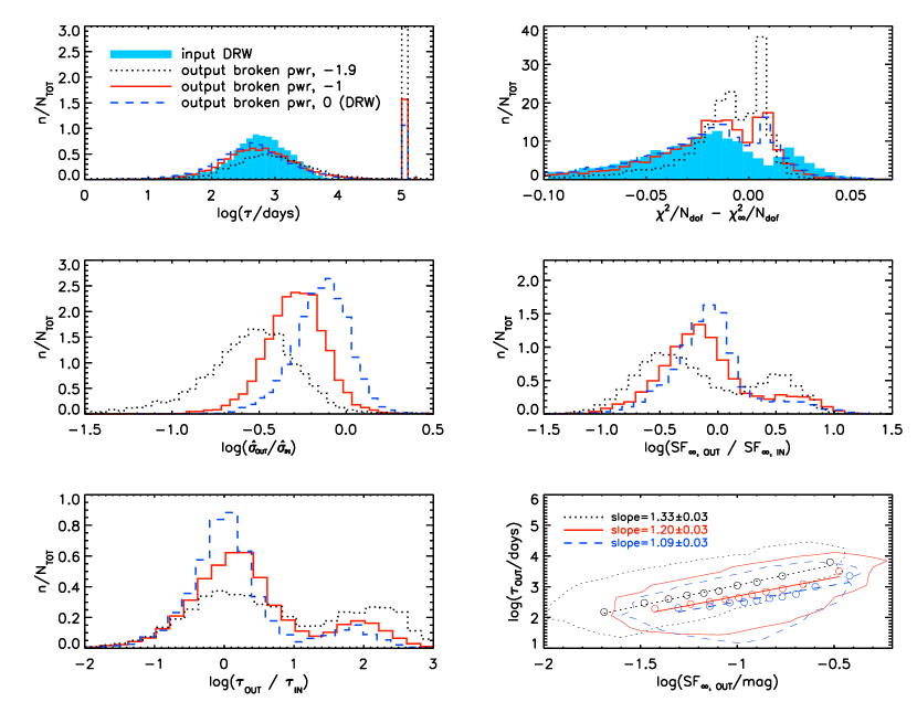
Each light curve was simulated over 100 years and then truncated to the 30–40 year segment in order to account for the additional variability and bias in the inferred $SF_{\infty}$, which may result from a red noise leak or an incorrect specification of the PSD model (see Uttley et al. 2002). The simulated light curves were then modeled as a damped random walk to obtain the (“output”) parameter distributions shown in Figures 10 and 11. For Figure 10, the simulated observations are spaced every 5 days over 10 years with typical errors of 0.01 mag, and for Figure 11, the S82 window function is imposed (i.e., all light curves have the S82 time sampling and photometric accuracy). The filled histograms show the input distributions and are the same for both Figures.

It is clear from comparing the input and output parameter distributions that $\tau$ and $SF_{\infty}$ map simply onto the values of the power-spectral break time scale and amplitude. Indeed, the correlation between $\tau$ and $SF_{\infty}$ is preserved in the output distributions, as seen in the bottom-right panels of Figures 10 and 11. However, as seen in the top- and bottom-left panels, as the PSD slope at low $f$ steepens to $\alpha=-1.9$, the number of “run-away” time scales (where $\tau$ saturates at $10^{5}$ days) increase due to that fact that $\tau$ can no longer be constrained. Whereas for the S82 data, $\sim$20% of light curves were rejected as run-away cases (see step 3 of Section 3.1), for an $\alpha=-1.9$ PSD, the run-away fraction is 30%. This significant increase rules out the $\alpha=-1.9$ PSD as the correct model, as we do not see this large run-away fraction in the data. The fractions are similar for the $\alpha=-1$ and $\alpha=0$ cases, suggesting that the correct model has $-1<\alpha<0$. The increasing fraction of run-away $\tau$ with decreasing $\alpha$ allows one to distinguish between each PSD in the well-sampled case, as seen in the top-right panel of Figure 10. In this panel, the difference between the $\chi^{2}_{pdf}$ for the best-fit damped random walk and that for a $\tau\rightarrow\infty$ solution, $\Delta\chi^{2}_{\infty}=\chi^{2}/N_{dof}-\chi^{2}_{\infty}/N_{dof}$, is shown for each input PSD. The total distribution shows two peaks; that on the left corresponds to cases where the model is able to constrain $\tau$. For well-sampled light curves (Figure 10), the case with $\alpha=0$ (dashed line) yields an overall lower $\Delta\chi^{2}_{\infty}$ and therefore a more likely damped random walk fit, as expected. However, for the S82 sampling, it is difficult to distinguish between the red and blue lines ($\alpha=0$ and $-1$), and the (input) observed distribution is similar to both. Therefore, within the limited S82 sampling, we are unable to distinguish reliably between a damped random walk and a $1/f$ PSD on long time scales.

5 Dependence of Variability Parameters on Luminosity, Wavelength, Redshift, and Black Hole Mass

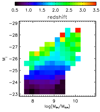
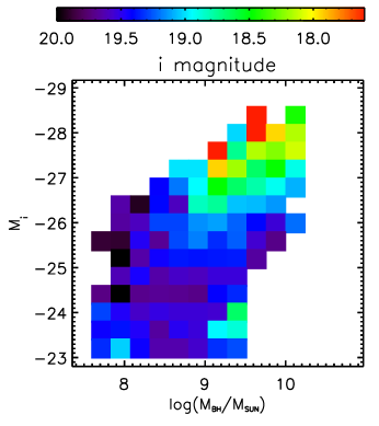
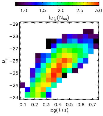
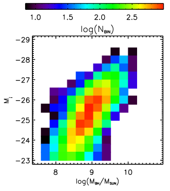
Next, we discuss correlations between each of the variability parameters, $\tau$ and $SF_{\infty}$, and the four available physical parameters: rest-frame wavelength ($\lambda_{RF}$), redshift ($z$), absolute i-band magnitude ($M_{i}$), and black hole mass ($M_{BH}$). It is important to fit a multiple regression to each of the physical parameters, functions of the form $\tau(\lambda_{RF},M_{i},M_{BH},z)$, because of the correlations between physical parameters. For example, when searching for a correlation between $SF_{\infty}$ and $M_{BH}$, one must take into account that a more luminous quasar hosts a more massive black hole (e.g., Kollmeier et al. 2006), or else a trend with luminosity may be mistaken for a trend with black hole mass. A similar example is the well-known luminosity-redshift ($L$–$z$) degeneracy seen in flux-limited samples of quasars. Magnitude limits result in the illusion that only the most luminous quasars are seen at high $z$, and therefore the observed $L$ increases with $z$ independent of reality. Having a large sample size helps to alleviate these degeneracies. For example, one can look for trends using 2-dimensional grids in any two physical parameters of interest. The numbers of data points per two-dimensional bin of $M_{i}$ and redshift, and similarly for $M_{i}$ and $M_{BH}$, are shown in the bottom panels of Figure 12. The two left panels of Figure 12 show the selection effect that quasars at higher redshift must have higher luminosities to be included in the survey. From the two-dimensional distribution in the top-left panel, we can see that this $L$–$z$ degeneracy is essentially independent of $M_{BH}$. Furthermore, shorter rest-frame wavelengths are probed at higher redshifts for two reasons: first, quasars emitting at shorter rest wavelengths must be at higher redshifts in order to be observed within the $ugriz$ filters, and second, quasars at high redshifts are closer to their Eddington limit as a result of the $L$–$z$ degeneracy, and possibly cosmological downsizing (e.g., Kollmeier et al. 2006). Therefore, any dependence of variability on wavelength must be accounted for when considering a dependence with redshift (or luminosity).

When fitting power laws to a large number of data points throughout this paper, we fit to the median values in each bin of the independent variable, where all bins have the same number of data points $N$. The errors in the medians are computed as 0.93(IQR)$/\sqrt{N-1}$, where IQR is the 25% – 75% interquartile range, and these constrain our formal errors in the power law slopes.

5.1 Trends with Rest-frame Wavelength

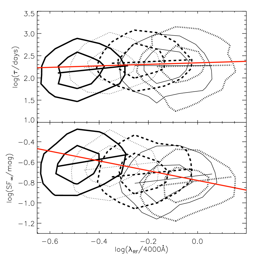
We start by examining the wavelength dependence of the variability parameters. Since there are multiple bands for each quasar, this dependence can be determined for individual sources for which $z$, $M_{i}$, and $M_{BH}$ are fixed. The rest-frame wavelength is found by dividing the observed bandpasses ($3520$, $4800$, $6250$, $7690$, and $9110$ Å for $ugriz$, respectively) by $(1+z)$. We fit a power law $f\propto(\lambda_{RF}/4000\AA)^{B}$ to the estimates of $\tau$ and $SF_{\infty}$ for every quasar observed in at least two filters ($\sim$8,000 quasars). The median values are $B=0.17\pm 0.02$ and $-0.479\pm 0.005$ for $\tau$ and $SF_{\infty}$, respectively. We searched for significant correlations between $B$ and other physical parameters and did not find any. We use these median values to correct for the wavelength dependence of $\tau$ and $SF_{\infty}$ before searching for their correlations with other physical parameters in Sections 5.2, 5.3, and 6.

This method of fixing $B$ before investigating other correlations naturally eliminates any degeneracies between rest wavelength and the other physical parameters. This is especially important in the case of the variability amplitude, $SF_{\infty}$. Figure 13 shows how the two variability parameters vary with $\lambda_{RF}$ in each of the $ugriz$ filters. The median power law from the above analysis, shown as a straight line stretching across all wavelengths, accurately traces the overall trend. However, when the data are fit to ensembles of quasars in each band separately, the slopes for $SF_{\infty}$, shown by the short lines for each filter, are very different ($\sim$0.4). This difference is a consequence of the correlation between $L$ and $z$: for a given band, shorter $\lambda_{RF}$ corresponds to higher $z$, but at higher $z$, quasars have higher $L$ and thus smaller $SF_{\infty}$ (see below), creating a bias in the inferred slope of the wavelength dependence.

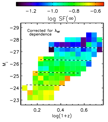
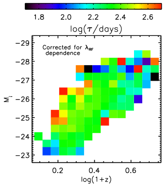
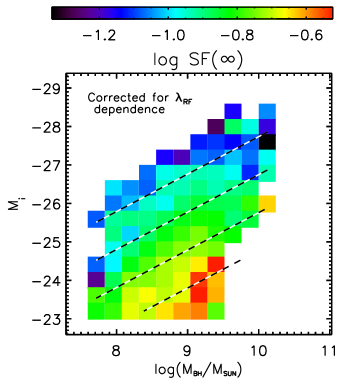
5.2 Trends with Luminosity, Redshift, and Black Hole Mass

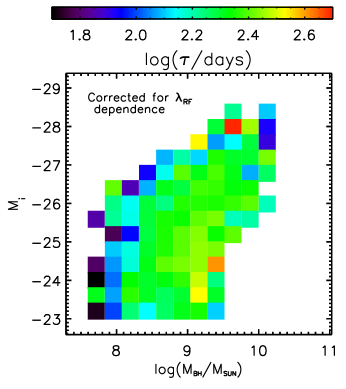
In the upper panels of Figure 14, the median values of $SF_{\infty}$ and $\tau$ are shown as a function of absolute magnitude ($M_{i}$) and redshift. The structure function parameters are normalized to a fixed rest wavelength of 4000Å using the fitted power law dependencies of $(\lambda_{RF}/4000\AA)^{B}$ with $B=-0.479$ and 0.17 for $SF_{\infty}$ and $\tau$, respectively, from Section 5.1, before finding the median in each pixel. For $SF_{\infty}$, the anti-correlation with luminosity clearly dominates any trend with redshift. The $\tau$ distribution also shows negligible correlation with redshift. The bottom panels show the dependence on $M_{BH}$. Using a grid of $M_{i}$ vs. $M_{BH}$ allows one to search for trends in the variability parameters while accounting for the selection effect that more luminous galaxies host more massive black holes. A positive correlation between $SF_{\infty}$ and $M_{BH}$ is apparent, independent of the correlation with $M_{i}$. This is in agreement with the result from Wilhite et al. (2008), who used ensemble structure functions. The $\tau$ parameter shows a clear correlation with $M_{BH}$, which dominates any trend with $M_{i}$.

Motivated by these qualitative results, we fit a power law of the form

$$\log{f}=A+B\log\left(\frac{\lambda_{RF}}{4000{\rm\AA}}\right)+C(M_{i}+23)+$$

$$D\log\left(\frac{M_{BH}}{10^{9}M_{\odot}}\right)+E\log(1+z),$$ (7)

to all $SF_{\infty}$ and $\tau$ data points in each $ugriz$ band separately, keeping $B$ fixed to $-0.479$ and $0.17$, respectively, in order to avoid the bias discussed in Section 5.1. While there is a lot of scatter in the variability parameters for fixed $M_{i}$, $M_{BH}$, and $\lambda_{RF}$ (see Section 4.2), Eq. 7 describes the mean trends well. The best-fit coefficients, averaged over the five bands, are reported in the first and sixth rows of Table 1. The best-fit coefficients when simultaneously fitting all bands are consistent with these averages. The reported error bars are computed from the variation of the best-fit parameters over the five bands.

The dependence of $\tau$ on redshift and $M_{i}$ is only marginally detected, and can be attributed to the $L$–$z$ degeneracy: as redshift increases, the best-fit $\tau$ decreases, while the coefficient for $M_{i}$ indicates that as luminosity increases, $\tau$ increases. When $E$ is fixed to zero, the dependence on $M_{i}$ has low significance, while the correlation with $M_{BH}$ remains the same (seventh row of Table 1). For illustration, when $E$ is fixed to 1 [so $\tau\propto(1+z)$, third and eighth rows], a spurious dependence on $M_{i}$ emerges. Therefore, the controlling variable for the characteristic time scale is clearly $M_{BH}$, suggesting that more massive black holes vary on longer time scales. Similarly, with $E$ fixed to 0 for $SF_{\infty}$ (second row), the $C$ ($M_{i}$) and $D$ ($M_{BH}$) coefficients remain largely unchanged, confirming that there is no significant correlation between amplitude and redshift. Therefore, we force the final adopted model to have no redshift dependence ($E=0$). Table 1 also provides fits for when $D$ is fixed to zero so that $SF_{\infty}$ and $\tau$ can be estimated in the absence of black hole mass information (fourth and ninth rows).

Of the analyzed parameters, the probable errors for black hole mass estimates are the largest: of order 0.2 – 0.4 dex (Marconi et al. 2008; Vestergaard & Peterson 2006). When ignored, these large statistical uncertainties result in underestimated values for $D$ (Kelly 2007). With an assumed random uncertainty of 0.2 dex in the black hole mass measurements, we find the best-fit coefficients reported in the fifth and tenth rows of Table 1 (continuing to assume that $E=0$). It can be seen that including mass uncertainties of 0.2 dex increases $D$ from $\sim$0.1 to $\sim$0.2 for both $\tau$ and $SF_{\infty}$ (a bias of about 2-3 formal statistical fitting errors). The coefficients in the fifth and tenth rows represent our best-fit model for the variability parameters, and we assume these values in the remaining Sections.

The best-fit model shows a smaller slope for the correlation between $\tau$ and $M_{BH}$ of $0.21\pm 0.07$ than the value of $1.0\pm 0.4$ found by KBS09. The two results are still marginally statistically consistent given the large uncertainties in KBS09. Moreover, their sample contains relatively lower mass and luminosity quasars than those analyzed in this study, and this difference might result in additional biases. Koz10 also noted that the KBS09 results may be affected by contamination from host galaxy emission, a problem which will be far smaller for the generally more luminous SDSS quasars.

Table 1: Best-Fit Coefficients for Eq. 7

$f$	$A$	$B$ ($\lambda_{RF}$)	$C$ ($M_{i}$)	$D$ ($M_{BH}$)	$E$ ($1+z$)
$SF_{\infty}$	$-0.57\pm 0.01$	$-0.479\pm 0.005$	$0.117\pm 0.009$	$0.11\pm 0.02$	$0.07\pm 0.05$
$SF_{\infty}$	$-0.56\pm 0.01$	$-0.479\pm 0.005$	$0.111\pm 0.005$	$0.11\pm 0.02$	$\equiv 0$
$SF_{\infty}$	$-0.760\pm 0.009$	$-0.479\pm 0.005$	$0.193\pm 0.006$	$0.12\pm 0.02$	$\equiv 1$
$SF_{\infty}$	$-0.618\pm 0.007$	$-0.479\pm 0.005$	$0.090\pm 0.003$	$\equiv 0$	$\equiv 0$
$SF_{\infty}$	$-0.51\pm 0.02$	$-0.479\pm 0.005$	$0.131\pm 0.008$	$0.18\pm 0.03$	$\equiv 0$
$\tau$	$\phantom{-0}2.4\pm 0.2\phantom{0}$	$\phantom{-0}0.17\pm 0.02\phantom{0}$	$-0.05\pm 0.03\phantom{0}$	$0.12\pm 0.04$	$-0.7\pm 0.5\phantom{-}$
$\tau$	$\phantom{-0}2.3\pm 0.1\phantom{0}$	$\phantom{-0}0.17\pm 0.02\phantom{0}$	$\phantom{-}0.01\pm 0.03\phantom{0}$	$0.12\pm 0.04$	$\equiv 0$
$\tau$	$\phantom{-0}2.1\pm 0.1\phantom{0}$	$\phantom{-0}0.17\pm 0.02\phantom{0}$	$\phantom{-}0.09\pm 0.03\phantom{0}$	$0.13\pm 0.04$	$\equiv 1$
$\tau$	$\phantom{-0}2.2\pm 0.1\phantom{0}$	$\phantom{-0}0.17\pm 0.02\phantom{0}$	$-0.01\pm 0.02\phantom{0}$	$\equiv 0$	$\equiv 0$
$\tau$	$\phantom{-0}2.4\pm 0.2\phantom{0}$	$\phantom{-0}0.17\pm 0.02\phantom{0}$	$\phantom{-}0.03\pm 0.04\phantom{0}$	$0.21\pm 0.07$	$\equiv 0$

Note. — In each row, the $B$ coefficient was determined and fixed before fitting a multiple regression in all other parameters (see Section 5.1). The cosmology used for determining $M_{i}$ is $\Omega_{M}=0.30$, $\Omega_{\Lambda}=0.70$, and $h=0.70$ (Schneider et al. 2007), whereas that used in the $M_{BH}$ estimates is $\Omega_{M}=0.26$, $\Omega_{\Lambda}=0.74$, and $h=0.71$ (Shen et al. 2008). This difference should only have a 1% effect on the best-fit coefficients.

5.3 The Eddington Ratio as the Driver of Variability?

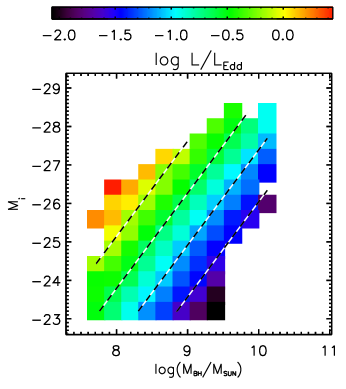
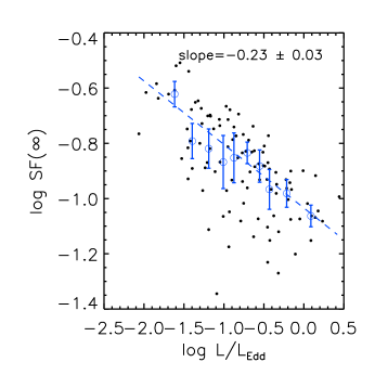
Since the Eddington ratio, $L/L_{Edd}$, is dependent on luminosity and black hole mass, the trends for $SF_{\infty}$ in Table 1 might be explained if $SF_{\infty}$ is simply driven by $L/L_{Edd}$. To test this, we estimated $L/L_{Edd}$ as the ratio of the bolometric luminosities from Shen et al. (2008) to the Eddington luminosity, $L_{Edd}=1.5\times 10^{38}(M_{BH}/M_{\odot})$ erg/s. Figure 15 shows $L/L_{Edd}$ as a function of $M_{BH}$ and $M_{i}$, and demonstrates that lines of constant $L/L_{Edd}$ are similar in slope to those of constant $SF_{\infty}$ (see Figure 14). The median $SF_{\infty}$ versus the median $L/L_{Edd}$ for each bin is shown in the right panel, where we find a power law slope of $-0.23\pm 0.03$. This significant anti-correlation was also found by Wilhite et al. (2008), Bauer et al. (2009), and Ai et al. (2010). KBS09 did not report such an anti-correlation; however, they did not compare $L/L_{Edd}$ with $SF_{\infty}$ but rather with $SF_{\infty}/\sqrt{\tau}$, the driving amplitude of short term variability. If $L/L_{Edd}$ is the sole driver of the quasar variability amplitude $SF_{\infty}$, we would expect that the coefficients for $M_{i}$ and $M_{BH}$ are related as $D=2.5C$. However, we find $D=(1.37\pm 0.23)C$, 4.7$\sigma$ away from the presumed slope of 2.5. This suggests an additional source of variability, such as a dependence on luminosity or on $M_{BH}$ in addition to the dependence on $L/L_{Edd}$. Moreover, if we ignore this additional source, the result that $SF_{\infty}$ depends on $L/L_{Edd}$ supports a scenario where the amplitude of the optical variability is determined by the accretion rate (see discussion in Wilhite et al. 2008).

If the Eddington ratio is a proxy for the quasar’s age (e.g., Martini & Schneider 2003), then a lower Eddington ratio, and thus a larger amplitude of variability, could indicate a dwindling fuel supply and a more variable rate at which it is supplied to the black hole. However, it is unlikely that the observed variability is due to fluctuations in the external fuel supply to the disk, because the fluctuation time scales of 10 – 10,000 days are very short compared to the viscous time scales of $10^{5}$ – $10^{7}$ days that should control large scale changes in the accretion rate. Moreover, these fluctuations in the fueling rate will also be smoothed out and damped as they travel inward, and will likely have effectively disappeared by the time they reach the optical emitting region (e.g., see discussion in Churazov et al. 2001). Instead, the origin of the fluctuations is probably more local.

Another possibility is that the dependence on $L/L_{Edd}$ may simply be a reflection of the dependence on wavelength, which in turn depends on the disk radius. If a higher $L/L_{Edd}$ means a hotter disk, then the optical flux originates at a larger radius. Assuming that longer wavelengths are emitted further out in the disk, the lower $SF_{\infty}$ at longer wavelengths would lead to the anti-correlation between $SF_{\infty}$ and $L/L_{Edd}$. In thin disk theory (e.g., see Frank, King, & Raine 2002), the characteristic radius for emission at wavelength $\lambda_{RF}$ scales as $R_{\lambda}\propto M_{BH}^{2/3}(L/L_{Edd})^{1/3}\lambda_{RF}^{4/3}$, and the thermal time scale is related to the orbital time scale as $t_{th}\propto t_{orb}\propto R^{3/2}/\sqrt{M_{BH}}$. Therefore, under the assumption that $\tau$ is related to the thermal time scale, and that variability at wavelength $\lambda_{RF}$ is dominated by the scale $R_{\lambda}$, $\tau$ scales with $\lambda_{RF}$, $M_{BH}$, and $L$ as:

$$\tau\propto M_{BH}^{1/2}(L/L_{Edd})^{1/2}\lambda_{RF}^{2}.$$ (8)

Since $L_{Edd}\propto M_{BH}$, this means $\tau$ scales as

$$\tau\propto L^{1/2}\lambda_{RF}^{2},$$ (9)

which does not match the observed scaling of $\tau\propto L^{-0.075}\lambda_{RF}^{0.17}M_{BH}^{0.21}$. If we assume that $\tau$ is related to the viscous time scale,

$$\tau\propto L^{7/60}\lambda_{RF}^{5/3}M_{BH}^{2/3},$$ (10)

still in conflict with the measured values.

The variability time scale simply does not show the strong dependence on $\lambda_{RF}$, $M_{BH}$, and $L$ expected from these simple scalings. Therefore, using this naive scaling, we are not able to relate the observed $\tau$ to either a thermal or viscous time scale of the radius associated with the wavelength of the variability. However, in reality there is a range of radii, which corresponds to a range in time scales, contributing to the observed flux in each band, and this will cause some degree of smoothing. Also, the radial regions might overlap for each band, causing a single radius to contribute flux in multiple bandpasses, and this might attenuate some of the dependencies on $\lambda_{RF}$, $M_{BH}$, and $L$. Finally, our observed power law indices may be biased due to the uncertainty in the bolometric correction.

5.4 A “Recipe” for Generating Mock Light Curves

Given the success of the damped random walk model in explaining a large body of observations, it represents a simple quantitative framework for generating mock quasar light curves. The optical light curves can be simulated for quasars at different redshifts and for a wide range of luminosity and black hole mass, which provides the basis for quantitative modeling and optimization of quasar variability surveys. The model presented has already been implemented as a part of the simulation effort in support of the Large Synoptic Survey Telescope (Ivezić et al. 2008).

At a given redshift, a simulated value for absolute magnitude can be readily drawn from an adopted luminosity function (e.g., Croom et al. 2009 and references therein). An estimate for the black hole mass is also required in order to apply our model, and it can be generated using the adopted absolute magnitude as follows. According to the Shen et al. (2008) results, the quasar luminosity and black hole mass are strongly correlated (see the bottom-right panel of Figure 12). Using Shen et al. (2008) values, we quantify this correlation in Figure 16. At a given $M_{i}$, the $M_{BH}$ distribution has a finite width due to the distribution of Eddington ratios and measurement errors. Both effects can be well-described using a Gaussian distribution:

$$p(\log{M_{BH}}|M_{i})=$$

$$\frac{1}{\sqrt{2\pi}\sigma}\exp\left[-\frac{(\log{M_{BH}}-\mu)^{2}}{2\sigma^{2}}\right],$$ (11)

where $\mu=2.0-0.27M_{i}$ and $\sigma=0.58+0.011M_{i}$ (the black hole mass is expressed in solar mass units).

With adopted values for $M_{i}$ and $M_{BH}$, the variability amplitude and the characteristic time scale can be estimated using Eq. 7. We note that choosing a time scale from an adopted value for $SF_{\infty}$ by utilizing the correlation seen in Figure 3 (and drawing from a Gaussian distribution similar to Eq. 5.4) is not as accurate as using Eq. 7 and the adopted values of $M_{BH}$ and $\lambda_{RF}$. Finally, given a mean magnitude and wavelength, a quasar light curve can be easily generated using Eq. 5.

6 Variability Properties of Radio- and X-ray–detected Quasars

Previous studies, based mostly on two-epoch datasets, found that radio-loud quasars are marginally more variable than radio-quiet quasars for rest-frame time lags in the range 50–400 days (e.g., VB04 and references therein). It was also found that X-ray–detected quasars are significantly more variable than X-ray–undetected quasars at rest-frame time lags up to 250 days.

The large size and the availability of light curves for our sample allows us to revisit these results with more statistical power. In addition, the damped random walk model and our best-fit results from Table 1 provide a convenient method to account for various selection effects. For example, it is possible that subsamples selected by various means, such as the requirement of radio or X-ray detections, have different distributions of luminosity and black hole mass. In this case, they would display different variability behavior not because of intrinsic differences in the variability mechanism, but rather because of the trends captured by Eq. 7. A comparison of the ratio of observed and predicted variability parameters for any subsample and the full sample will automatically take into account these sampling effects, and this is the main statistical method we use in this section. We first discuss a radio subsample, and then analyze a sample of quasars with X-ray detections.

6.1 Radio-detected Subsample

We use the unified radio catalog of Kimball & Ivezić (2008) to access the FIRST and NVSS data (20 cm continuum data) for our objects. We refer the reader to this paper and references therein for details about these radio surveys and object association. Figure 17 shows the radio-detected fraction of quasars in S82 as a function of magnitude. The overall fraction (5%) is considerably lower than that in the Northern galactic cap footprint of the SDSS for the magnitude range $19<i<20$ (White et al. 1997; Ivezić et al. 2002). This is due to a difference in targeting algorithms between the two surveys, and results in nearly 300 quasars with both optical light curves and radio data. When available, we use NVSS values for radio flux, but otherwise we adopt the FIRST integrated flux. The radio-loudness parameter $R_{g}$ is calculated exactly as the $R_{i}$ in Ivezić et al. (2002), but using $g$ magnitudes instead. We assume a spectral index of $-0.5$ for the optical and 0 for the radio (because this sample is dominated by the core radio emission; see Kimball & Ivezić 2008) when computing the K-correction.

Table 2 compares the mean properties for various subsamples detected in the radio to the radio-undetected subsample (essentially the full sample due to small fraction of radio-detected objects). For each subsample, the mean $\tau$ and $SF_{\infty}$ are listed, as well as the mean ratio of the observed values to those predicted using Eq. 7 and the measured values of $\lambda_{RF}$, $M_{i}$, and $M_{BH}$. The mean values are computed iteratively with $\pm 3\sigma$ outliers excluded. Errors are reported as the (clipped) rms divided by $\sqrt{N-1}$, where N is the number of data points in the distribution. Numbers of objects are lower for columns involving model quantities because black hole mass estimates are not available for all objects.

Table 2 shows that only the variability amplitude of the radio-loudest quasar subsample ($R_{g}\geq 3$) is significantly different ($>3\sigma$ deviation) from the behavior of the full sample. The radio-loudest quasars have systematically larger variability amplitudes, when corrected for trends described by Eq. 7, by about 30%, compared to the full sample dominated by radio-quiet objects, in agreement with VB04.

6.2 X-ray Detected Subsample

For the analysis of variability properties of quasars detected at X-ray wavelengths, we use data from the ROSAT All-Sky Survey (RASS; Voges et al. 1999). The X-ray subsample consists of 82 quasars with RASS full-band count rates greater than $10^{-3}$ ct/s, taken from the Schneider et al. (2007) catalog. As can be seen from Table 2, the variability properties of this subsample are statistically indistinguishable from the full sample. VB04 detected a significant increase in structure function at rest time lags below 250 days for their X-ray subsample, but on long time scales there was no significant difference. It is plausible that their result for short time scales was influenced by small sample size and $\tau$ effects discussed in Section 4.3.

Table 2: Mean Variability Properties of Radio and X-ray Subsamples

	$\small{<}\log\tau\small{>}$	$N$	$\small{<}\log(\tau/\tau_{p})\small{>}$	$N$	$\small{<}\log SF_{\infty}\small{>}$	$N$	$\small{<}\log(SF_{\infty}/SF_{\infty,p})\small{>}$	$N$
no radio	$2.305\pm 0.005$	6989	$-0.003\pm 0.007$	4467	$-0.634\pm 0.003$	7067	$0.018\pm 0.003$	4508
no radio $i<19$	$2.327\pm 0.013$	1519	$-0.013\pm 0.013$	1279	$-0.721\pm 0.006$	1527	$0.003\pm 0.006$	1287
radio	$2.26\pm 0.03$	277	$-0.07\pm 0.05$	154	$-0.70\pm 0.02$	283	$-0.03\pm 0.02\phantom{-}$	154
radio $i<19$	$2.24\pm 0.06$	105	$-0.08\pm 0.06$	73	$-0.81\pm 0.03$	108	$-0.08\pm 0.03\phantom{-}$	74
$R_{g}\geq 3$	$2.30\pm 0.05$	135	$-0.01\pm 0.07$	68	$-0.57\pm 0.02$	137	${\bf 0.11\pm 0.03}$	68
$R_{g}<3$	$2.28\pm 0.03$	211	$\phantom{-}0.00\pm 0.04$	133	$-0.73\pm 0.02$	219	$-0.06\pm 0.02\phantom{-}$	140
$R_{g}<2$	$1.99\pm 0.14$	30	$-0.21\pm 0.14$	19	$-0.88\pm 0.07$	30	$-0.12\pm 0.06\phantom{-}$	19
resolved	$2.29\pm 0.05$	111	$\phantom{-}0.00\pm 0.06$	63	$-0.63\pm 0.02$	111	$0.04\pm 0.03$	63
unresolved	$2.24\pm 0.04$	167	$-0.13\pm 0.07$	91	$-0.73\pm 0.03$	172	$-0.06\pm 0.03\phantom{-}$	91
x-ray	$2.41\pm 0.05$	81	$\phantom{-}0.03\pm 0.06$	59	$-0.60\pm 0.03$	82	$0.01\pm 0.03$	58
no x-ray	$2.307\pm 0.005$	6950	$-0.004\pm 0.007$	4559	$-0.638\pm 0.003$	7020	$0.017\pm 0.003$	4598

Note. — $\tau$ and $SF_{\infty}$ are the observed time scales and asymptotic amplitudes of optical variability (Section 4), while $\tau_{p}$ and $SF_{\infty,p}$ refer to those predicted from Eq. 7, using the coefficients in the fifth and the tenth rows of Table 1. Errors are reported as the rms divided by $\sqrt{N-1}$, where N is the number of data points, listed after each column. Numbers of objects are lower for columns involving model estimates because black hole mass estimates are not available for all objects. Only the variability amplitude for the radio-loudest quasar subsample ($R_{g}\geq 3$) is significantly different ($>3\sigma$ deviation) from the behavior of the full sample.

7 Summary and Conclusions

We have used the damped random walk model of KBS09 and Koz10 to model the optical/UV variability of $\sim$9000 SDSS Stripe 82 quasars with the $ugriz$ light curves. The dataset includes 2.7 million photometric measurements collected over 10 years. We confirm that this is a good model of quasar variability, and quantify the dependence of two variability parameters, the long-term rms variability $SF_{\infty}$ and the damping time scale $\tau$, on physical parameters such as wavelength, luminosity, black hole mass and Eddington ratio. Our main results are the following:

1. A stochastic process with an exponential covariance function characterized by an amplitude and time scale provides a good fit to observed quasar light curves, as shown by KBS09 and Koz10, using smaller samples with less wavelength coverage, but better time sampling.

2. The long-term rms variability, $SF_{\infty}$, has a mode at $\sim$0.2 mag and characteristic time scales, $\tau$, are roughly 200 days in the rest frame, as found previously by KBS09 and Koz10. These time scales are consistent with thermal time scales, but simple accretion disk models fail to reproduce the observed scaling of $\tau$ with physical parameters.

3. Quasars with similar physical parameters can have different characteristic time scales for variability. It is now clear that the distribution of $\tau$ accounts for most of the scatter in the structure function on short time scales for quasars with similar luminosity, rest wavelength, and time lag, which explains the puzzling results from MacLeod et al. (2008). Results from fitting a power law to observed ensemble structure functions should be interpreted with caution.

4. The variability time scale is correlated with the long-term rms variability with a slope of $1.30\pm 0.01$ dex/dex. Quasars that have large long-term variability amplitudes generally vary on longer characteristic time scales. The amplitude of short term variations is also correlated with $\tau$. This conclusion is unaffected by any time sampling issues in the S82 dataset.

5. The damped random walk corresponds to a PSD proportional to $1/f^{2}$ at frequencies $f>(2\pi\tau)^{-1}$, flattening to a constant at lower frequencies. At large $f$, the data are in great agreement with $PSD\propto 1/f^{2}$. In terms of the structure function, this means that $SF\propto(\Delta t)^{1/2}$. Whereas previous analyses of the SF obtained a power law slope of $\beta=0.3$, here we demonstrated that this would be a consequence of fitting the data around the “knee” (turn-over) of the SF. Our constraints for small $f$ are much weaker. As discussed in Section 4.4, due to a lack of sufficient long-time scale information, we are unable to distinguish between a $1/f^{0}$ or a $1/f$ PSD at frequencies $f<(2\pi\tau)^{-1}$ using the data and computational technique described here.

6. The rest-frame variability parameters show a negligible trend with redshift, suggesting that they are intrinsic to the quasars, and these properties do not evolve over cosmic time for fixed physical parameters of the quasar ($M_{BH}$, $M_{i}$, and $\lambda_{RF}$).

7. For fixed luminosity and black hole mass, $\tau$ increases with increasing rest-frame wavelength with a power law index of $0.17$, and $SF_{\infty}$ decreases with a power law index of $-0.48$. The latter result is similar to previous findings (e.g., MacLeod et al. 2008, VB04). Koz10 also observed that the variability increases to shorter $\lambda$, but they kept $\tau$ fixed in their fits. If wavelength is a proxy for radius in the accretion disk, this implies that the characteristic time scales are longer and the variability amplitudes are smaller in the outer regions than in the inner regions.

8. The long-term variability $SF_{\infty}$ is strongly anti-correlated with luminosity as found in previous studies such as VB04, Wilhite et al. (2008), and references therein. By studying the median $SF_{\infty}$ in the plane of absolute magnitude and black hole mass, we can separate the anti-correlation of amplitude with luminosity from the positive correlation with black hole mass. As suggested in Wilhite et al. (2008), these trends may be largely explained if the amplitude of variability is tied to changes in the accretion rate in the disk, and is simply related to the Eddington ratio. However, despite the strong anti-correlation between $SF_{\infty}$ and $L/L_{Edd}$ (which accounts for most of the dependence on $M_{i}$ and $M_{BH}$), the exact dependence with $M_{i}$ and $M_{BH}$ is not consistent with $L/L_{Edd}$ as the sole driver of quasar variability.

9. The damping time scale $\tau$ appears to be nearly independent of luminosity and correlated with $M_{BH}$ with a power law index of $0.21\pm 0.07$. The mild discrepancy with the KBS09 result (1.0$\pm$0.4) may be due to the different range of sampled luminosity and black hole mass, as well as contamination by host galaxy emission in many of the very low luminosity systems they consider (see Koz10).

10. While the mean variability parameters can be related to physical parameters, for fixed values of $M_{i}$, $\lambda_{RF}$, and $M_{BH}$, there is still a large scatter around the mean values, similar to the variance of the observed distributions. Some of that scatter can be attributed to measurement and fitting errors ($\sim$60% for $\tau$ and $\sim$70% for $SF_{\infty}$), but there is enough evidence for residual stochastic nature of quasar variability. Therefore, it cannot be assumed that quasars with similar $M_{i}$, $\lambda_{RF}$, and $M_{BH}$ will necessarily have similar variability properties.

11. The radio-loudest quasars have systematically larger variability amplitude by about 30%, while the distribution of their characteristic time scale is indistinguishable from that of the full sample. There are no statistically robust differences in the characteristic time scale and variability amplitude between the full sample and a small subsample of quasars detected by ROSAT.

With this paper, and results from KBS09 and Koz10, the ability of the damped random walk model to quantitatively describe quasar variability is well-established. As emphasized by Koz10, this means that variability studies can become fully quantitative because the entire process of identifying and assigning parameters to quasars can be simulated to allow estimates of completeness and parameter biases. In particular, an important next step is to determine the variability equivalents of luminosity functions, i.e., the intrinsic distributions of the variability parameters. While our results represent a good first step in this direction, we caution that a non-negligible fraction of the S82 quasars have indeterminately long time scales. If, following KBS09, we identify the characteristic time scale with the thermal time scale, then the next question is whether there are additional time scales (such as the dynamical or viscous time scale), or sources of variability. For example, Blackburne & Kochanek (2010) recently found evidence for changes in disk size with changes in luminosity using gravitational microlensing. Such searches for additional sources of variability will likely require better sampled light curves and over a longer time scale.

The prospect of advancing these studies of quasar variability now faces a bottleneck. The S82 quasars have the advantage of sample size, wavelength coverage, and spectroscopy, but the light curves have poor sampling and modest overall lengths, leading to significant problems for accurately estimating $\tau$ when it is long. The quasars behind the Magellanic Clouds (Kozłowski & Kochanek 2009) are a smaller sample without spectroscopic confirmation, but have superb, long term light curves that continue to be extended because of the continuing microlensing projects. Improving on our present results in the short term depends on either reviving the monitoring of S82 or spectroscopically confirming the Magellanic Cloud quasars.

Resuming the monitoring of Stripe 82 is challenging with the decommissioning of the SDSS imaging system. The best short-term prospects are the Pan-STARRS project (Kaiser et al. 2002), the Palomar-QUEST project (Schweitzer et al. 2006), or using the DECam being built for the Dark Energy Survey (Honscheid et al. 2008). Since the challenge is to constrain long time scales, the presence of a multiple-year gap is mainly a complication for ensuring that problems in matching photometric bands are not interpreted as a form of long-term variability. Obtaining spectra of the Magellanic Cloud quasars is in some ways easier, because the quasar magnitudes and densities are well-suited to the AAOmega fiber spectrograph on the AAT and, to a lesser degree, the IMACS spectrograph on Magellan.

The more general, Northern monitoring projects such as Pan-STARRS and Palomar-QUEST will slowly build light curves for essentially all the SDSS quasars, but at present their cadences are not ideal (see Schmidt et al. 2010) and it will take nearly a decade to build the long duration light curves needed for the analysis. In the long term, observations will be significantly improved with the advent of next-generation sky surveys. Most notably, the Large Synoptic Survey Telescope (LSST, Ivezić et al. 2008) will obtain accurate, well-sampled light curves for millions of AGN. The observed distribution of rest-frame characteristic time scales for S82 quasars spans the range from about 10 days to 1000 days (c.f. Figure 3). To probe the time scales as short as $0.1\tau$, and assuming a characteristic redshift of 2, the light curves should be sampled every 3 days in the observer’s frame, which is in good agreement with the baseline cadence of LSST. With a 10 year-long survey, the length of the light curves will be in the range (1-200)$\tau$. A combination of the SDSS, Pan-STARRS, DES, and LSST data for $\sim$10,000 Stripe 82 quasars would span well over two decades, with multi-band photometry obtained for hundreds of epochs, and would represent the best sample to date for studying the optical continuum variability of quasars. In particular, such a dataset would enable a robust measurement of the low-frequency behavior of their PSD (c.f. point 5 above). For illustration, the LSST photometric errors in the $r$ band will be $<0.02$ mag for $r<22$, and there are roughly 2-3 million AGN with $r<22$ in the 20,000 sq. deg. covered by the main LSST survey (see Table 10.2 in the LSST Science Book; Abell et al. 2009). Each of these objects will be observed about 1000 times, yielding a database of over 2 billion photometric measurements. This data set, roughly a thousand times larger than that analyzed here, will enable a significant improvement in our understanding of quasar variability.

Appendix: Search for Periodic Light Curves

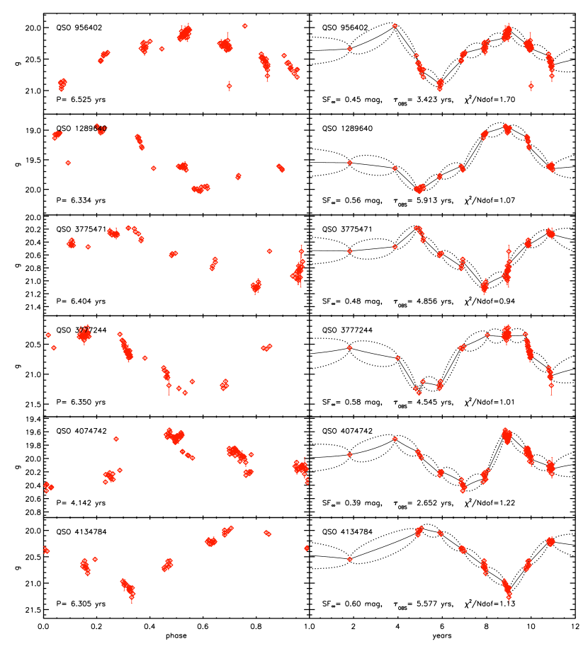
Although a stochastic process has proven to be an accurate statistical description of quasar light curves, any discovery of periodic behavior (even of a single source) would have interesting physical implications. However, a periodogram can only be used as an indicator of significant periodicity in a signal as compared to pure white noise (i.e., having no signal at all). Since quasars are genuinely variable, as described by a damped random walk (i.e., a red noise process; see KBS09), one can only evaluate the significance of the periodicity when also allowing for the signal covariance that is also present (see Markwardt et al. 2009; Gotz et al. 2009; Cenko et al. 2009, and references therein). Nevertheless, as a quick test for outstanding cases of periodicity among the S82 light curves, we analyzed 8,863 light curves for evidence of periodicity using the Lomb-Scargle periodogram (Lomb 1976; Scargle 1982). The threshold for considering the strongest peak in the periodogram as candidate evidence for periodicity was set following Horne & Baliunas (1986), with an adopted false alarm probability of 0.05. However, this is the threshold for ruling out white noise in favor of periodicity, and therefore provides no information on how a periodic description compares to a colored noise process such as a damped random walk. To determine the latter, a different threshold is needed (see Koz10). When adopting the threshold for ruling out white noise in favor of periodic variability, we identify 88 light curves as good candidates.

A close inspection of the period distribution for the full sample and the selected 88 candidates shows important differences: while the full sample displays a fairly flat distribution ranging from 100 days to values exceeding 10,000 days, the period distribution for 88 candidates is bimodal. The first peak with 22 objects corresponds to aliasing at roughly one-year sampling cadence, while the second peak is centered on periods of about 6-7 years, similar to the total length of observations. We have visually inspected the light curves and phased light curves for all 88 candidates. It turns out that candidates with proposed periods of the order one year have light curves consistent with aliasing, while those with longer periods typically have only one observed “oscillation” that might not be used as robust evidence for periodicity (six examples are shown in Figure 18). Therefore, our search for periodic light curves in the S82 quasar sample has not yielded any convincing cases. Again, it is important to note that in cases such as in Figure 18, the periodogram indicates that these sources with long $\tau$ are likely to be periodic, not because they show true periodicity, but because it computes the likelihood relative to the wrong null hypothesis (white noise rather than colored noise). Moreover, the fact that $<$5% of the light curves exceed the threshold for periodicity being a better description than pure white noise is a further indication that the periodogram is not a very powerful statistic for poorly sampled light curves, since it is clear from the previous Sections that quasar light curves are not white noise, but rather are well described by a damped random walk. In fact, the single “oscillation” observed for the best candidate long period objects is entirely expected from colored noise processes such as a damped random walk (see right panels of Figure 18). Therefore, this analysis is further evidence that a damped random walk is a good description of quasar light curves.

Figure 1: The top panel shows a segment of a simulated light curve with $\tau=20$ days and $SF_{\infty}=0.10$ mag. In the bottom panel, triangles, squares, and crosses represent the SF computed for the first, second, and third sections of the total light curve, respectively (each has a length of $500\tau$). The increased scatter in $SF(\Delta t)$ at large time lags is due to the finite length of each light curve section – the scatter decreases when using the entire light curve length of $1500\tau$ (as shown by the solid line). The short-dashed line is a power law fit, $SF(\Delta t)\propto\Delta t^{\beta}$ with $\beta=0.3$, to the data points with $0.15<\Delta t/\tau<3$. The long-dashed line is the true function $SF=SF_{\infty}[1-e^{-\Delta t/\tau}]^{1/2}$.

Figure 2: Initial light curve selection. Top-left: the distribution of the number of observations per light curve for the $r$ (solid) and $u$ (dashed) bands. Top-right: distribution of $\Delta L_{noise}$. We define light curves with $\Delta L_{noise}\leq 2$ to be more consistent with uncorrelated noise rather than our model. Bottom-left: distribution of $\Delta L_{\infty}$; light curves with $\Delta L_{\infty}\leq 0.05$ likely have run-away time scales. In this panel and the previous panel, the x-axes are truncated at $0.5$ and $5$ respectively, but the histograms continue to greater values. Bottom-right: distribution of $\chi^{2}$ per degrees of freedom ($N_{dof}$) for the damped random walk model (solid line). The expected Gaussian distribution based on $N_{dof}$ is also shown (dashed). The hashed region in each panel shows the values rejected from our final sample.

Figure 3: Top: Distributions of the best-fit rest-frame time scale $\tau$ (left) and long-term structure function $SF_{\infty}$ (right) for the S82 quasars ($33,112$ light curves). The filled histograms show the fits for quasars with absolute i-band magnitude in the range $-27<M_{i}<-26$ (the median $M_{i}$ for the whole sample is $-25.46$). Bottom: Relationship between $\tau$ and $SF_{\infty}$. A power law shown by the dashed line is fit to the medians (open white circles), with the slope listed in the top-right corner. Contours show regions containing 90%, 70%, 50%, and 20% of the total number of points. The star symbols label the four regions in parameter space from which the sample light curves in Fig. 4 (labeled A through D) were chosen. The observed-frame $\tau$ distribution lacks many of the short time scales observed in Koz10. This is likely due to either the better time sampling of the OGLE light curves or stellar contamination in their sample.

Figure 4: Each panel shows a sample light curve from a certain region of $\tau$, $SF_{\infty}$ space (the four regions A–D are indicated with stars in the bottom panel of Figure 3). Data points with error bars show the observed S82 data. Solid lines show the weighted average of the damped random walk model light curves that are consistent with the data (see Section 2). Dotted lines show the $\pm 1\sigma$ range of these possible stochastic models about the average.

Figure 5: Test of biases in best-fit parameters. Left: The input variability parameters $\tau$ and $SF_{\infty}$ were drawn from a uniform distribution in $\log\tau$ and $\log SF_{\infty}$ limited by the dotted rectangle. The contours show the output distribution after applying the cuts described in Section 3.1, and the dashed line is a linear regression between the output parameters (with the slope listed on the panel). Solid, blue circles show the objects which do not satisfy $\Delta L_{\infty}>0.05$ (these make up 21% of the starting sample, where 13% are saturated at $\tau=10^{5}$ days). The small black dots show the input values for these rejected points. Open, red circles show the 3% that do not satisfy $\Delta L_{noise}>2$. Right: Relationship between $\tau_{out}$/$\tau_{in}$ and $SF_{out}$/$SF_{in}$. The slope of the cleaned output distribution is listed. The sharp edge is due to the saturation limit of $\tau=10^{5}$ days. The contours show the 90%, 70%, 50%, and 20% levels.

Figure 6: Top panel: Data points with error bars show the observed light curve for a quasar in our final sample, the solid line shows the weighted average of all consistent model light curves, and the dotted lines show the $\pm 1\sigma$ range of possible stochastic models (see Section 2). Bottom panel: A “regenerated” light curve using Eq. 5 and the estimated values of $\tau$ and $SF_{\infty}$ listed in the top panel. Due to the poor time sampling of the light curve, the best fit to the “regenerated” light curve has a run-away time scale (listed at the bottom), with $\Delta L_{\infty}=0.003$.

Figure 7: Results from “regenerating” light curves derived from the observed $\tau$ and $SF_{\infty}$ (see Section 4.2). The solid, black lines in the top panels show the distribution of input $SF_{\infty}$ (left) and $\tau$ (right) normalized by the median input value, and the ratio of output to input values are shown by the red, dashed lines. The bottom panels show the scatter in the output-to-input ratios (left), and the relationship between the output parameters (right). Listed in each bottom panel is the slope of a linear fit (dashed line) to the median values (open circles). Contours show the 90%, 70%, 50%, and 20% levels.

Figure 8: The symbols with error bars show the distribution of $SF_{obs}/SF_{model}$ from Figure 2 in MacLeod et al. (2008), where $SF_{obs}$ is the observed structure function for individual S82 light curves for a fixed observed-frame time lag of 1 year, and $SF_{model}=1(1+0.03M_{i})(\Delta t_{RF}/\lambda_{RF})^{0.47}$. The distribution from the ensemble analysis by I04 (based on two-epoch SDSS data) is shown by the dashed curve, scaled by a factor of 0.2. The dotted histogram is the distribution of $\sqrt{\rm median(\tau)/\tau}$ from this work, where $\tau$ is the characteristic time scale for each light curve. Its agreement with the $SF_{obs}/SF_{model}$ distribution for individual light curves shows that most of the scatter pointed out by MacLeod et al. (2008) is due to a finite width of the $\tau$ distribution.

Figure 9: First three panels: Simulated light curves using $\tau=5.8$ days, $rms=0.124$ mag, and a PSD described by $PSD\propto f^{\alpha}$, with $\alpha=-2$ for $f>(2\pi\tau)^{-1}$, and $\alpha=-1$ (red; top-left), $\alpha=0$ (blue; top-right), or $\alpha=-1.9$ (green; bottom-left) for $f<(2\pi\tau)^{-1}$. The lines in the last panel show each PSD from which the light curves are generated, with the black dotted line indicating the break frequency. As a check, the PSD was then computed for the simulated light curves, shown with colored dots. The y-axis in the bottom-right panel is in arbitrary units.

Figure 10: In the top panels, the filled histogram shows the (“input”) distributions of $\tau$ and $\Delta\chi^{2}_{\infty}=\chi^{2}/N_{dof}-\chi^{2}_{\infty}/N_{dof}$ for $r$-band S82 light curves ($\sim$7000 total). This distribution of $\tau$, along with the $r$-band $rms$ values, are used to generate $\sim$7000 realizations of noise processes with $\alpha=-2$ for $f>(2\pi\tau)^{-1}$ and $\alpha=0$, $\alpha=-1$, or $\alpha=-1.9$ for $f<(2\pi\tau)^{-1}$. The dashed blue, solid red, and dotted lines show the best-fit (“output”) distributions when modeling these three processes, respectively, as a damped random walk (DRW). Here, the simulated observations are spaced every 5 days over 10 years with typical errors of 0.01 mag. The output $\hat{\sigma}$, $SF_{\infty}$, and $\tau$ are compared to the input values in the next three panels. In the last panel, the correlation between the output $log(SF_{\infty})$ and $log(\tau)$ is shown using a linear fit to the median values (open circles), with the slopes listed in the legend for each case. Contours show regions containing 90% of the data points.

Figure 11: As in Figure 10, except with the Stripe 82 time sampling and photometric accuracy imposed on the simulated light curves.

Figure 12: The top panels show the distribution of quasars in redshift (left) and i magnitude (right) on a grid of $M_{BH}$ vs. $M_{i}$. The bottom panels show the number of data points in bins of $M_{BH}$ (or redshift) vs. $M_{i}$.

Figure 13: Distribution of the rest-frame time scale $\tau$ (top panel) and long-term structure function $SF_{\infty}$ (bottom panel) as a function of rest-frame wavelength $\lambda_{RF}$. The different contours show the 70% and 30% levels for the $u$, $g$, $r$, $i$, and $z$ (from left to right) bands. The best-fit power law for each subsample is shown with the same line style as the contours. The thick red line connecting the left and right axes shows the median power law slope derived by fitting individual quasars (see text), and has a value of $B=0.17$ and $-0.479$ for $\tau$ and $SF_{\infty}$, respectively. The slope within each band from fitting ensembles of quasars can be quite different from the overall slope because of the $L$–$z$ degeneracy (see text).

Figure 14: Top panels: The long-term rms variability $SF_{\infty}$ (left) and characteristic time scale $\tau$ (right) are shown as colors on a grid of redshift and absolute i-band magnitude $M_{i}$. The structure function parameters are normalized to a fixed rest wavelength using the fitted power law dependencies of $(\lambda_{RF}/4000\AA)^{B}$ with $B=-0.479$ and 0.17 for $SF_{\infty}$ and $\tau$, respectively. The lines of constant variability (dashed) show that $SF_{\infty}$ is independent of redshift. Bottom panels: As in the top panels but with black hole mass $M_{BH}$ on the x-axis.

Figure 15: Left: The Eddington ratio for S82 quasars (estimated using masses and bolometric luminosities from Shen et al. 2008) is shown as colors on a grid of $M_{i}$ vs. $M_{BH}$, with dashed lines of constant $L/L_{Edd}$ over-plotted. Right: Long-term rms variability (corrected for wavelength dependence) is shown as a function of $L/L_{Edd}$ (open circles are medians in each bin). The slope of the linear fit to the medians is listed on the panel.

Figure 16: Determination of $p(M_{BH}|M_{i})$ (see Eq. 5.4). The histograms in the top three panels show the distribution of black hole masses for S82 quasars with absolute magnitudes within $0.5$ mags of the value listed in the upper right corners. In the bottom panel, the mean value of $\log{(M_{BH}/M_{\odot})}$ from each histogram is plotted against $M_{i}$.

Figure 17: Top: The number of FIRST radio detections (thick line, multiplied by 10) as compared to the total number of quasars (thin line) as a function of $i$ magnitude in the Northern galactic cap (NGC) footprint of the SDSS. Middle: As in the top panel but for Stripe 82. Bottom: Fraction of quasars in the NGC (thin line) and in S82 (thick line) samples that have radio detections. Between $i=19$ and 20, the fraction of radio-detected quasars is considerably lower in S82 than in the NGC.

Figure 18: Six examples of candidate light curves showing significant periodicity as compared to pure noise (see Appendix). The phased light curves are shown on the left, where the phase is the fractional part of the ratio of time to the period (i.e., the phase zero-point is arbitrary). The best-fit period is listed on the bottom of each panel. The full light curves are shown on the right, where the solid lines show the weighted average of all consistent damped random walk model light curves, and the dotted lines show the $\pm 1\sigma$ range of possible stochastic models (see Section 2). The best-fit damped random walk parameters are listed at the bottom of the right panels, along with the reduced $\chi^{2}$.

References

- Abazajian et al. (2009) Abazajian, K. N., et al. 2009, ApJS, 182, 543
- LSST Science Collaborations: Paul A. Abell et al. (2009) Abell, P. A. et al. 2009, arXiv:0912.0201; http://www.lsst.org/lsst/scibook
- Ai et al. (2010) Ai, Y. L., Yuan, W., Zhou, H. Y., Wang, T. G., Dong, X. -., Wang, J. G., & Lu, H. L. 2010, arXiv:1005.0901
- Aretxaga et al. (1997) Aretxaga, I., Cid Fernandes, R., & Terlevich, R. J. 1997, MNRAS, 286, 271
- Arévalo et al. (2008b) Arévalo, P., Uttley, P., Kaspi, S., Breedt, E., Lira, P., & McHardy, I. M. 2008b, MNRAS, 389, 1479
- Arévalo et al. (2008a) Arévalo, P., McHardy, I. M., & Summons, D. P. 2008a, MNRAS, 388, 211
- Bauer et al. (2009) Bauer, A., Baltay, C., Coppi, P., Ellman, N., Jerke, J., Rabinowitz, D., & Scalzo, R. 2009, ApJ, 696, 1241
- Bhatti et al. (2010) Bhatti, W. A., Richmond, M. W., Ford, H. C., & Petro, L. D. 2010, ApJS, 186, 233
- Blackburne & Kochanek (2010) Blackburne, J. A., & Kochanek, C. S. 2010, arXiv:1002.3126
- Cenko et al. (2009) Cenko, S. B., et al. 2009, arXiv:0911.3150
- Churazov et al. (2001) Churazov, E., Gilfanov, M., & Revnivtsev, M. 2001, MNRAS, 321, 759
- Collier & Peterson (2001) Collier, S., & Peterson, B. M. 2001, ApJ, 555, 775
- Croom et al. (2009) Croom, S.M., Richards, G.T., Shanks, T., et al. 2009, MNRAS, 399, 1755
- Denney et al. (2009) Denney, K. D., Peterson, B. M., Dietrich, M., Vestergaard, M., & Bentz, M. C. 2009, ApJ, 692, 246
- de Vries et al. (2005) de Vries, W. H., Becker, R. H., White, R. L., & Loomis, C. 2005, AJ, 129, 615
- Emmanoulopoulos et al. (2010) Emmanoulopoulos, D., McHardy, I. M., & Uttley, P. 2010, arXiv:1001.2045
- Frank et al. (2002) Frank, J., King, A., & Raine, D. J. 2002, Accretion Power in Astrophysics (Cambridge, UK: Cambridge University Press)
- Fukugita et al. (1996) Fukugita, M., Ichikawa, T., Gunn, J.E., Doi, M., Shimasaku, K., & Schneider, D.P. 1996, AJ, 111, 1748
- Geha et al. (2003) Geha, M., et al. 2003, AJ, 125, 1
- Gotz et al. (2009) Gotz, D., Mereghetti, S., von Kienlin, A., & Beck, M. 2009, GRB Coordinates Network, 9649, 1
- Gunn et al. (1998) Gunn, J.E., et al. 1998, AJ, 116, 3040
- Giveon et al. (1999) Giveon, U., Maoz, D., Kaspi, S., Netzer, H., & Smith, P. S. 1999, MNRAS, 306, 637
- Hawkins (1993) Hawkins, M. R. S. 1993, Nature, 366, 242
- Hawkins (2007) Hawkins, M. R. S. 2007, A&A, 462, 581
- Honscheid et al. (2008) Honscheid, K., DePoy, D. L., & for the DES Collaboration 2008, arXiv:0810.3600
- Hook et al. (1994) Hook, I. M., McMahon, R. G., Boyle, B. J., & Irwin, M. J. 1994, MNRAS, 268, 305
- (27) Horne, J.H., & Baliunas, S.L. 1986, ApJ, 302, 757
- Hughes et al. (1992) Hughes, P. A., Aller, H. D., & Aller, M. F. 1992, ApJ, 396, 469
- Ivezić et al. (2002) Ivezić, Ž., et al. 2002, AJ, 124, 2364
- Ivezić et al. (2004) Ivezić, Ž., et al. 2004, The Interplay Among Black Holes, Stars and ISM in Galactic Nuclei, 222, 525 [I04]
- Ivezić et al. (2007) Ivezić, Ž., et al. 2007, AJ, 134, 973
- Ivezić et al. (2008) Ivezić, Ž., Tyson, J. A., Allsman, R., Andrew, J., Angel, R., & for the LSST Collaboration 2008, arXiv:0805.2366
- Kaiser et al. (2002) Kaiser, N., et al. 2002, Proc. SPIE, 4836, 154
- Kawaguchi et al. (1998) Kawaguchi, T., Mineshige, S., Umemura, M., & Turner, E. L. 1998, ApJ, 504, 671
- Kelly (2007) Kelly, B. C. 2007, ApJ, 665, 1489
- Kelly et al. (2009) Kelly, B. C., Bechtold, J., & Siemiginowska, A. 2009, ApJ, 698, 895 [KBS09]
- Kimball & Ivezić (2008) Kimball, A. E., & Ivezić, Ž. 2008, AJ, 136, 684
- Kollmeier et al. (2006) Kollmeier, J. A., et al. 2006, ApJ, 648, 128
- Kozłowski & Kochanek (2009) Kozłowski, S., & Kochanek, C. S. 2009, ApJ, 701, 508
- Kozłowski et al. (2010) Kozłowski, S., et al. 2010a, ApJ, 708, 927 [Koz10]
- Kozłowski et al. (2010) Kozłowski, S., et al. 2010b, arXiv:1002.3365
- Li & Cao (2008) Li, S.-L., & Cao, X. 2008, MNRAS, 387, L41
- Liu et al. (2008) Liu, H. T., Bai, J. M., Zhao, X. H., & Ma, L. 2008, ApJ, 677, 884
- (44) Lomb, N.R. 1976, Ap&SS, 39, 447
- MacLeod et al. (2008) MacLeod, C., Ivezić, Ž., de Vries, W., Sesar, B., & Becker, A. 2008, American Institute of Physics Conference Series, 1082, 282
- Marconi et al. (2008) Marconi, A., Axon, D. J., Maiolino, R., Nagao, T., Pastorini, G., Pietrini, P., Robinson, A., & Torricelli, G. 2008, ApJ, 678, 693
- Markwardt et al. (2009) Markwardt, C. B., Gavriil, F. P., Palmer, D. M., Baumgartner, W. H., & Barthelmy, S. D. 2009, GRB Coordinates Network, 9645, 1
- Martini & Schneider (2003) Martini, P., & Schneider, D. P. 2003, ApJ, 597, L109
- Matthews & Sandage (1963) Matthews, T. A., & Sandage, A. R. 1963, ApJ, 138, 30
- McHardy (2010) McHardy, I. 2010, Lecture Notes in Physics, Berlin Springer Verlag, 794, 203
- Pereyra et al. (2006) Pereyra, N. A., Vanden Berk, D. E., Turnshek, D. A., Hillier, D. J., Wilhite, B. C., Kron, R. G., Schneider, D. P., & Brinkmann, J. 2006, ApJ, 642, 87
- Peterson et al. (2005) Peterson, B. M., et al. 2005, ApJ, 632, 799
- Press et al. (1992) Press, W. H., Rybicki, G. B., & Hewitt, J. N. 1992, ApJ, 385, 404
- Rengstorf et al. (2006) Rengstorf, A. W., Brunner, R. J., & Wilhite, B. C. 2006, AJ, 131, 1923
- Rybicki & Press (1992) Rybicki, G. B., & Press, W. H. 1992, ApJ, 398, 169
- Rybicki & Press (1994) Rybicki, G. B., & Press, W. H. 1994, Computer, 5004
- (57) Scargle, J.D. 1982, ApJ, 263, 835
- Schmidt et al. (2010) Schmidt, K. B., Marshall, P. J., Rix, H.-W., Jester, S., Hennawi, J. F., & Dobler, G. 2010, arXiv:1002.2642
- Schneider et al. (2007) Schneider, D. P., et al. 2007, AJ, 134, 102
- Schweitzer et al. (2006) Schweitzer, M., et al. 2006, ApJ, 649, 79
- Sesar et al. (2006) Sesar, B., et al. 2006, AJ, 131, 2801
- Sesar et al. (2007) Sesar, B., et al. 2007, AJ, 134, 2236
- Shen et al. (2008) Shen, Y., Greene, J. E., Strauss, M. A., Richards, G. T., & Schneider, D. P. 2008, ApJ, 680, 169
- Smith et al. (2002) Smith, J. A., et al. 2002, AJ, 123, 2121
- Timmer & Koenig (1995) Timmer, J., & Koenig, M. 1995, A&A, 300, 707
- Trèvese et al. (2001) Trèvese, D., Kron, R. G., & Bunone, A. 2001, ApJ, 551, 103
- Trèvese & Vagnetti (2002) Trèvese, D., & Vagnetti, F. 2002, ApJ, 564, 624
- Udalski et al. (1997) Udalski et al. 1997, Acta Astron 47 319
- Udalski et al. (2008) Udalski et al. 2008, Acta Astron 58 69
- Uttley et al. (2002) Uttley, P., McHardy, I. M., & Papadakis, I. E. 2002, MNRAS, 332, 231
- Vanden Berk et al. (2004) Vanden Berk, D. E., et al. 2004, ApJ, 601, 692 [VB04]
- Vestergaard & Peterson (2006) Vestergaard, M., & Peterson, B. M. 2006, ApJ, 641, 689
- Voges et al. (1999) Voges, W., et al. 1999, A&A, 349, 389
- White et al. (1997) White, R. L., Becker, R. H., Helfand, D. J., & Gregg, M. D. 1997, ApJ, 475, 479
- Wilhite et al. (2005) Wilhite, B. C., Vanden Berk, D. E., Kron, R. G., Schneider, D. P., Pereyra, N., Brunner, R. J., Richards, G. T., & Brinkmann, J. V. 2005, ApJ, 633, 638
- Wilhite et al. (2006) Wilhite, B. C., Vanden Berk, D. E., Brunner, R. J., & Brinkmann, J. V. 2006, ApJ, 641, 78
- Wilhite et al. (2008) Wilhite, B. C., Brunner, R. J., Grier, C. J., Schneider, D. P., & Vanden Berk, D. E. 2008, MNRAS, 383, 1232
- Wold et al. (2007) Wold, M., Brotherton, M. S., & Shang, Z. 2007, MNRAS, 375, 989
- York et al. (2000) York, D.G. et al. 2000, AJ, 120, 1579