Diagnosis and Prediction of Market Rebounds in Financial Markets

Abstract

We introduce the concept of “negative bubbles” as the mirror (but not necessarily exactly symmetric) image of standard financial bubbles, in which positive feedback mechanisms may lead to transient accelerating price falls. To model these negative bubbles, we adapt the Johansen-Ledoit-Sornette (JLS) model of rational expectation bubbles with a hazard rate describing the collective buying pressure of noise traders. The price fall occurring during a transient negative bubble can be interpreted as an effective random down payment that rational agents accept to pay in the hope of profiting from the expected occurrence of a possible rally. We validate the model by showing that it has significant predictive power in identifying the times of major market rebounds. This result is obtained by using a general pattern recognition method that combines the information obtained at multiple times from a dynamical calibration of the JLS model. Error diagrams, Bayesian inference and trading strategies suggest that one can extract genuine information and obtain real skill from the calibration of negative bubbles with the JLS model. We conclude that negative bubbles are in general predictably associated with large rebounds or rallies, which are the mirror images of the crashes terminating standard bubbles.

Keywords: negative bubble, rebound, positive feedback, pattern recognition, trading strategy, error diagram, prediction, Bayesian methods, financial markets, price forecasting, econophysics, complex system, critical point phenomena

I Introduction

Financial bubbles are generally defined as transient upward acceleration of prices above fundamental value Galbraith (1997); Kindleberger (2000); Sornette (2003). However, identifying unambiguously the presence of a bubble remains an unsolved problem in standard econometric and financial economic approaches Gurkaynak (2008); Lux and Sornette (2002), due to the fact that the fundamental value is in general poorly constrained and it is not possible to distinguish between exponentially growing fundamental price and exponentially growing bubble price.

To break this stalemate, Sornette and co-workers have proposed that bubbles are actually not characterized by exponential prices (sometimes referred to as “explosive”), but rather by faster-than-exponential growth of price (that should therefore be referred to as “super-explosive”). See Sornette (2003) and references therein. The reason for such faster-than-exponential regimes is that imitation and herding behavior of noise traders and of boundedly rational agents create positive feedback in the valuation of assets, resulting in price processes that exhibit a finite-time singularity at some future time $t_{c}$. See Goriely and Hyde (2000) for a general theory of finite-time singularities in ordinary differential equations, Gluzman and Sornette (2002) for a classification and Johansen and Sornette (2001a); Sammis and Sornette (2002); Sornette et al. (2003) for applications. This critical time $t_{c}$ is interpreted as the end of the bubble, which is often but not necessarily the time when a crash occurs Johansen and Sornette (2006). Thus, the main difference with standard bubble models is that the underlying price process is considered to be intrinsically transient due to positive feedback mechanisms that create an unsustainable regime. Furthermore, the tension and competition between the value investors and the noise traders may create deviations around the finite-time singular growth in the form of oscillations that are periodic in the logarithm of the time to $t_{c}$. Log-periodic oscillations appear to our clocks as peaks and valleys with progressively greater frequencies that eventually reach a point of no return, where the unsustainable growth has the highest probability of ending in a violent crash or gentle deflation of the bubble. Log-periodic oscillations are associated with the symmetry of discrete scale invariance, a partial breaking of the symmetry of continuous scale invariance, and occurs in complex systems characterized by a hierarchy of scales. See Sornette (1998) for a general review and references therein.

Recent literatures on bubbles and crashes can be summarized as the following kinds: first, the combined effects of heterogeneous beliefs and short-sales constraints may cause large movements in asset. In this kind of models, the asset prices are determined at equilibrium to the extent that they reflect the heterogeneous beliefs about payoffs. But short sales restrictions force the pessimistic investors out of the market, leaving only optimistic investors and thus inflated asset price levels. However, when short sales restrictions no longer bind investors, then prices fall back down Lintner (1969); Miller (1977); Harrison and Kreps (1978); Jarrow (1980); Chen et al. (2002); Scheinkman and Xiong (2003); Duffie et al. (2002); Abreu and Brunnermeier (2003). While in the second type, the role of “noise traders” in fostering positive feedback trading has been emphasized. These models says trend chasing by one class of agents produces momentum in stock prices DeLong et al. (1990); Barberis et al. (1998); Daniel et al. (1998); Hong et al. (2005). The empirical evidence on momentum strategies can be found in Jegadeesh and Titman (1993, 2001); Bondt and Thaler (1985).

After the discussion on bubbles and crashes, the literatures on rebound should be summarized also. On the theoretical side, there are several competing explanations for price decreases followed by reversals: liquidity and time-varying risk. Pedersen (2009) stresses the importance of liquidity: as more people sell, agents who borrowed money to buy assets are forced to sell too. When forced selling stops, this trend reverses. Nagel (2010) shows that it is risky to be a fundamental trader in this environment and that price reversals after declines are likely to be higher when there is more risk in the price, as measured by volatility. On the empirical front concerning the forecast of reversals in price drops, Jegadeesh and Titman (1993) shows that the simplest way to predict prices is to look at past performance. Campbell and Shiller (1988) shows that price-dividend ratios forecast future returns for the market as a whole. However, these two approaches do not aim at predicting and cannot determine the most probable rebound time for a single ticker of the stock. The innovation of our methodology in this respect is to provide a very detailed method to detect rebound of any given ticker.

In this paper, we explore the hypothesis that financial bubbles have mirror images in the form of “negative bubbles” in which positive feedback mechanisms may lead to transient accelerating price falls. We adapt the Johansen-Ledoit-Sornette (JLS) model of rational expectation bubbles Johansen and Sornette (1999); Johansen et al. (1999, 2000) to negative bubbles. The crash hazard rate becomes the rally hazard rate, which quantifies the probability per unit time that the market rebounds in a strong rally. The upward accelerating bullish price characterizing a bubble, which was the return that rational investors require as a remuneration for being exposed to crash risk, becomes a downward accelerating bearish price of the negative bubble, which can be interpreted as the cost that rational agents accept to pay to profit from a possible future rally. During this accelerating downward trend, a tiny reversal could be a strong signal for all the investors who are seeking the profit from the possible future rally. These investors will long the stock immediately after this tiny reversal. As a consequence, the price rebounds very rapidly.

This paper contributes to the literature by augmenting the evidence for transient pockets of predictability that are characterized by faster-than-exponential growth or decay. This is done by adding the phenomenology and modeling of “negative bubbles” to the evidence for characteristic signatures of (positive) bubbles. Both positive and negative bubbles are suggested to result from the same fundamental mechanisms, involving imitation and herding behavior which create positive feedbacks. By such a generalization within the same theoretical framework, we hope to contribute to the development of a genuine science of bubbles.

The rest of the paper is organized as follows. Section 2.1 summarizes the main definitions and properties of the Johansen-Ledoit-Sornette (JLS) for (positive) bubbles and their associated crashes. Section 2.2 presents the modified JLS model for negative bubbles and their associated rebounds (or rallies). The subsequent sections test the JLS model for negative bubbles by providing different validation steps, in terms of prediction skills of actual rebounds and of abnormal returns of trading strategies derived from the model. Section 3 describes the method we have developed to test whether the adapted JLS model for negative bubbles has indeed skills in forecasting large rebounds. This method uses a robust pattern recognition framework build on the information obtained from the calibration of the adapted JLS model to the financial prices. Section 4 presents the results of the tests concerning the performance of the method of section 3 with respect to the advanced diagnostic of large rebounds. Section 5 develops simple trading strategies based on the method of section 3, which are shown to exhibit statistically significant returns, when compared with random strategies without skills with otherwise comparable attributes. Section 6 concludes.

II Theoretical model for detecting rebounds

II.1 Introduction to the JLS model and bubble conditions

Johansen and Sornette (1999), Johansen et al. (1999), Johansen et al. (2000) developed a model (referred to below as the JLS model) of financial bubbles and crashes, which is an extension of the rational expectation bubble model of Blanchard and Watson (1982). In this model, a crash is seen as an event potentially terminating the run-up of a bubble. A financial bubble is modeled as a regime of accelerating (super-exponential power law) growth punctuated by short-lived corrections organized according the symmetry of discrete scale invariance Sornette (1998). The super-exponential power law is argued to result from positive feedback resulting from noise trader decisions that tend to enhance deviations from fundamental valuation in an accelerating spiral.

In the JLS model, the dynamics of stock markets is described as

$$\frac{dp}{p}=\mu(t)dt+\sigma(t)dW-\kappa dj~{},$$ (1)

where $p$ is the stock market price, $\mu$ is the drift (or trend) and $dW$ is the increment of a Wiener process (with zero mean and unit variance). The term $dj$ represents a discontinuous jump such that $dj=0$ before the crash and $dj=1$ after the crash occurs. The loss amplitude associated with the occurrence of a crash is determined by the parameter $\kappa$. The assumption of the constant jump size is easily relaxed by considering a distribution of jump sizes, with the condition that its first moment exists. Then, the no-arbitrage condition is expressed similarly with $\kappa$ replaced by its mean. Each successive crash corresponds to a jump of $dj$ by one unit. The dynamics of the jumps is governed by a crash hazard rate $h(t)$. Since $h(t)dt$ is the probability that the crash occurs between $t$ and $t+dt$ conditional on the fact that it has not yet happened, we have $E_{t}[dj]=1\times h(t)dt+0\times(1-h(t)dt)$ and therefore

$${\rm E}_{t}[dj]=h(t)dt~{}.$$ (2)

Under the assumption of the JLS model, noise traders exhibit collective herding behaviors that may destabilize the market. The JLS model assumes that the aggregate effect of noise traders can be accounted for by the following dynamics of the crash hazard rate

$$h(t)=B^{\prime}(t_{c}-t)^{m-1}+C^{\prime}(t_{c}-t)^{m-1}\cos(\omega\ln(t_{c}-t)-\phi^{\prime})~{}.$$ (3)

The intuition behind this specification (3) has been presented at length in Johansen and Sornette (1999); Johansen et al. (1999, 2000), among others, and further developed in (Sornette and Johansen, 2002) for the power law part and by Ide and Sornette (2002) and (Zhou et al., 2005) for the second term in the right-hand-side of expression (3). In a nutshell, the power law behavior $\sim t_{c}-t)^{m-1}$ embodies the mechanism of positive feedback posited to be at the source of the bubbles. If the exponent $m<1$, the crash hazard may diverge as $t$ approaches a critical time $t_{c}$, corresponding to the end of the bubble. The cosine term in the r.h.s. of (3) takes into account the existence of a possible hierarchical cascade of panic acceleration punctuating the course of the bubble, resulting either from a preexisting hierarchy in noise trader sizes Sornette and Johansen (1997) and/or from the interplay between market price impact inertia and nonlinear fundamental value investing Ide and Sornette (2002).

The no-arbitrage condition reads ${\rm E}_{t}[dp]=0$, where the expectation is performed with respect to the risk-neutral measure, and in the frame of the risk-free rate. This is the standard condition that the price process is a martingale. Taking the expectation of expression (1) under the filtration (or history) until time $t$ reads

$${\rm E}_{t}[dp]=\mu(t)p(t)dt+\sigma(t)p(t){\rm E}_{t}[dW]-\kappa p(t){\rm E}_{t}[dj]~{}.$$ (4)

Since ${\rm E}_{t}[dW]=0$ and ${\rm E}_{t}[dj]=h(t)dt$ (equation (2)), together with the no-arbitrage condition ${\rm E}_{t}[dp]=0$, this yields

$$\mu(t)=\kappa h(t)~{}.$$ (5)

This result (5) expresses that the return $\mu(t)$ is controlled by the risk of the crash quantified by its crash hazard rate $h(t)$.

Now, conditioned on the fact that no crash occurs, equation (1) is simply

$$\frac{dp}{p}=\mu(t)dt+\sigma(t)dW=\kappa h(t)dt+\sigma(t)dW~{}.$$ (6)

Its conditional expectation leads to

$${\rm E}_{t}\left[\frac{dp}{p}\right]=\kappa h(t)dt~{}.$$ (7)

Substituting with the expression (3) for $h(t)$ and integrating yields the so-called log-periodic power law (LPPL) equation:

$$\ln{\rm E}[p(t)]=A+B(t_{c}-t)^{m}+C(t_{c}-t)^{m}\cos(\omega\ln(t_{c}-t)-\phi)$$ (8)

where $B=-\kappa B^{\prime}/m$ and $C=-\kappa C^{\prime}/\sqrt{m^{2}+\omega^{2}}$. Note that this expression (8) describes the average price dynamics only up to the end of the bubble. The JLS model does not specify what happens beyond $t_{c}$. This critical $t_{c}$ is the termination of the bubble regime and the transition time to another regime. This regime could be a big crash or a change of the growth rate of the market. Merrill Lynch EMU (European Monetary Union) Corporates Non-Financial Index in 2009 Sornette et al. (2010a) provides a vivid example of a change of regime characterized by a change of growth rate rather than by a crash or rebound. For $m<1$, the crash hazard rate accelerates up to $t_{c}$ but its integral up to $t$ which controls the total probability for a crash to occur up to $t$ remains finite and less than $1$ for all times $t\leq t_{c}$. It is this property that makes it rational for investors to remain invested knowing that a bubble is developing and that a crash is looming. Indeed, there is still a finite probability that no crash will occur during the lifetime of the bubble. The excess return $\mu(t)=\kappa h(t)$ is the remuneration that investors require to remain invested in the bubbly asset, which is exposed to a crash risk. The condition that the price remains finite at all time, including $t_{c}$, imposes that $m>0$.

Within the JLS framework, a bubble is qualified when the crash hazard rate accelerates. According to (3), this imposes $m<1$ and $B^{\prime}>0$, hence $B<0$ since $m>0$ by the condition that the price remains finite. We thus have a first condition for a bubble to occur

$$0<m<1~{}.$$ (9)

By definition, the crash rate should be non-negative. This imposes v. Bothmer and Meister (2003)

$$b\equiv-Bm-|C|\sqrt{m^{2}+\omega^{2}}\geq 0~{}.$$ (10)

II.2 Modified JLS model for “negative bubbles” and rebounds

As recalled above, in the JLS framework, financial bubbles are defined as transient regimes of faster-than-exponential price growth resulting from positive feedbacks. We refer to these regimes as “positive bubbles.” We propose that positive feedbacks leading to increasing amplitude of the price momentum can also occur in a downward price regime and that transient regimes of faster-than-exponential downward acceleration can exist. We refer to these regimes as “negative bubbles.” In a “positive” bubble regime, the larger the price is, the larger the increase of future price. In a “negative bubble” regime, the smaller the price, the larger is the decrease of future price. In a positive bubble, the positive feedback results from over-optimistic expectations of future returns leading to self-fulfilling but transient unsustainable price appreciations. In a negative bubble, the positive feedbacks reflect the rampant pessimism fueled by short positions leading investors to run away from the market which spirals downwards also in a self-fulfilling process.

The symmetry between positive and negative bubbles is obvious for currencies. If a currency A appreciates abnormally against another currency B following a faster-than-exponential trajectory, the value of currency B expressed in currency A will correspondingly fall faster-than-exponentially in a downward spiral. In this example, the negative bubble is simply obtained by taking the inverse of the price, since the value of currency A in units of B is the inverse of the value of currency B in units of A. Using logarithm of prices, this corresponds to a change of sign, hence the “mirror” effect mentioned above.

The JLS model provides a suitable framework to describe negative bubbles, with the only modifications that both the expected excess return $\mu(t)$ and the crash amplitude $\kappa$ become negative (hence the term “negative” bubble). Thus, $\mu$ becomes the expected (negative) return (i.e., loss) that investors accept to bear, given that they anticipate a potential rebound or rally of amplitude $|\kappa|$. Symmetrically to the case of positive bubbles, the price loss before the potential rebound plays the role of a random payment that the investors honor in order to remain invested and profit from the possible rally. The hazard rate $h(t)$ now describes the probability per unit time for the rebound to occur. The fundamental equations (3) and (8) then hold mutatis mutandis with the inequalities

$$B>0~{},~{}~{}~{}~{}b<0$$ (11)

being the opposite to those corresponding to a positive bubble as described in the preceding subsection.

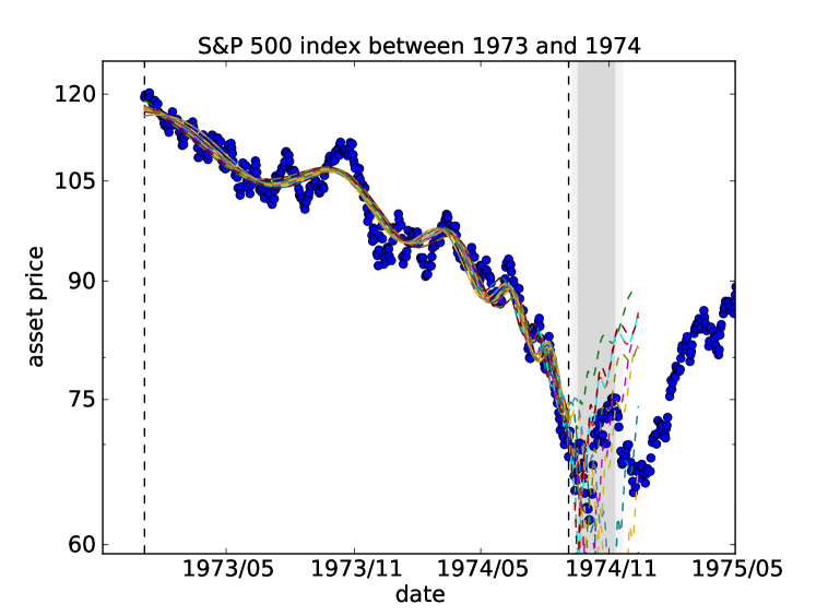
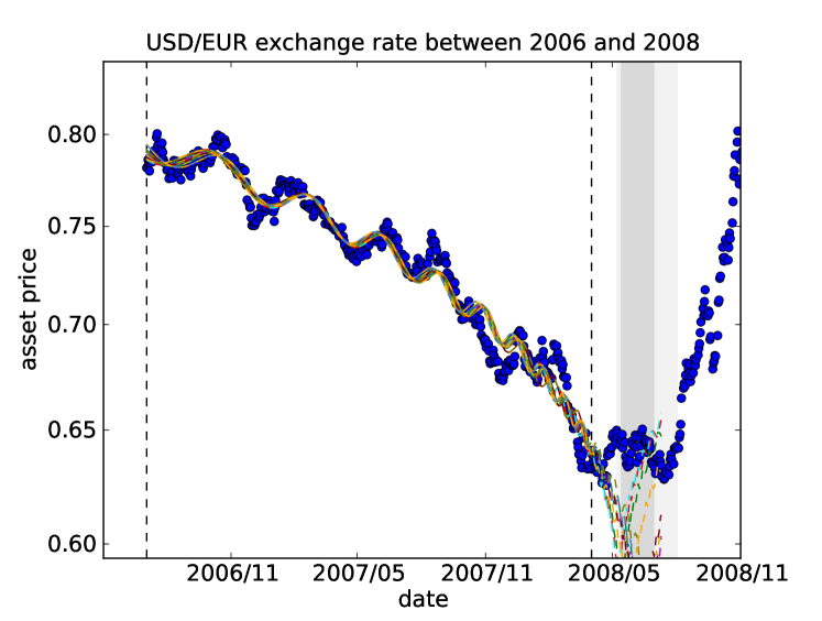
An example of the calibration of a negative bubble with the JLS model (4) to the S&P 500 index from 1973-01-01 to 1974-10-01 is shown in the upper panel of Figure 1. During this period, the S&P 500 index decreased at an accelerating pace. This price fall was accompanied by very clear oscillations that are log-periodic in time, as described by the cosine term in formula (4). Notice that the end of the decreasing market is followed by a dramatic rebound in index price. We hypothesize that, similar to a crash following an unsustainable super-exponential price appreciation (a positive bubble), an accelerating downward price trajectory (a negative bubble) is in general followed by a strong rebound. Furthermore, in order to suggest that this phenomenon is not an isolated phenomenon but actually happens widely in all kinds of markets, another example in the foreign exchange market is presented in the lower panel of Figure 1. The USD/EUR change rate from 2006-07-01 to 2008-04-01 also underwent a significant drawdown with very clear log-periodic oscillations, followed by a strong positive rebound. One of the goals of this paper is to identify such regions of negative bubbles in financial time series and then use a pattern recognition method to distinguish ones that were (in a back-testing framework) followed by significant price rises.

In financial markets, large positive returns are less frequent than large negative returns, as expressed for instance in the skewness of return distributions. However, when studying drawdowns and drawups (i.e., runs of same sign returns). Johansen and Sornette found that, for individual companies, there are approximately twice as many large rallies as crashes with amplitude larger than 20% with durations of a few days Johansen and Sornette (2001b).

III Rebound prediction method

We adapt the pattern recognition method of Gelfand et al. (1976) to generate predictions of rebound times in financial markets on the basis of the detection and calibration of negative bubbles, defined in the previous section. We analyze the S&P 500 index prices, obtained from Yahoo! finance for ticker ‘^GSPC’ (adjusted close price). The start time of our time series is 1950-01-05, which is very close to the first day when the S&P 500 index became available (1950-01-03). The last day of our tested time series is 2009-06-03.

III.1 Fitting methods

We first divide our S&P 500 index time series into different sub-windows $(t_{1},t_{2})$ of length $dt\equiv t_{2}-t_{1}$ according to the following rules:

1. The earliest start time of the windows is $t_{1}=$ 1950-01-03. Other start times $t_{1}$ are calculated using a step size of $dt_{1}=50$ calendar days.

2. The latest end time of the windows is $t_{2}=$ 2009-06-03. Other end times $t_{2}$ are calculated with a negative step size $dt_{2}=-50$ calendar days.

3. The minimum window size $dt_{\mathrm{min}}=110$ calendar days.

4. The maximum window size $dt_{\mathrm{max}}=1500$ calendar days.

These rules lead to 11,662 windows in the S&P 500 time series.

For each window, the log of the S&P 500 index is fit with the JLS equation (8). The fit is performed in two steps. First, the linear parameters $A,B$ and $C$ are slaved to the non-linear parameters by solving them analytically as a function of the nonlinear parameters. We refer to Johansen et al. (2000) (page 238 and following ones), which gives the detailed equations and procedure. Then, the search space is obtained as a 4 dimensional parameter space representing $m,\omega,\phi,t_{c}$. A heuristic search implementing the Tabu algorithm Cvijovic and Klinowski (1995) is used to find initial estimates of the parameters which are then passed to a Levenberg-Marquardt algorithm Levenberg (1944); Marquardt (1963) to minimize the residuals (the sum of the squares of the differences) between the model and the data. The bounds of the search space are:

$$m \in [0.001,0.999]$$ (12)

$$\omega \in [0.01,40]$$ (13)

$$\phi \in [0.001,2\pi]$$ (14)

$$t_{c} \in [t_{2},t_{2}+0.375(t_{2}-t_{1})]$$ (15)

We choose these bounds because $m$ has to be between $0$ and $1$ according to the discussion before; the log-angular frequency $\omega$ should be greater than $0$. The upper bound $40$ is large enough to catch high-frequency oscillations (though we later discard fits with $\omega>20$); phase $\phi$ should be between 0 and $2\pi$; as we are predicting a critical time in financial markets, the critical time should be after the end of the time series we are fitting. Finally, the upper bound of the critical time should not be too far away from the end of the time series since predictive capacity degrades far beyond $t_{2}$. We have empirically found elsewhere Jiang et al. (2010) one-third of the interval width to be a good cut-off.

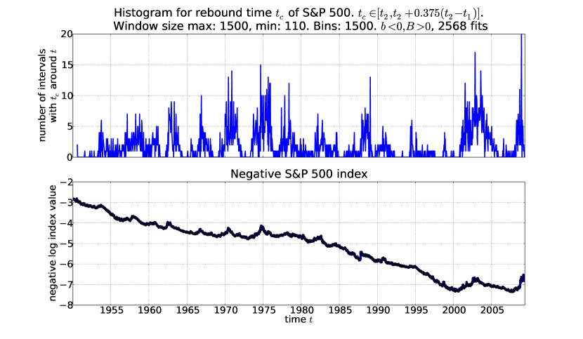
The combination of the heuristic and optimization results in a set of parameters $A,B,C,m,\omega,\phi$ and $t_{c}$ for each of the 11,662 windows. Of these parameter sets, 2,568 satisfy the negative bubble condition (11). In Figure 2, we plot the histogram of critical time $t_{c}$ for these negative bubble fits and the negative logarithm of the S&P 500 time series. Peaks in this time series, then, indicate minima of the prices, many of these peaks being preceded by a fast acceleration with upward curvature indicating visually a faster-than-exponential growth of $-p(t)$. This translates into accelerating downward prices. Notice that many of these peaks of $-\ln p(t)$ are followed by sharp drops, that is, fast rebounds in the regular $+\ln p(t)$. We see that peaks in $-\ln p(t)$ correspond to peaks in the negative bubble $t_{c}$ histogram, implying that the negative bubbles qualified by the JLS model are often followed by rebounds. This suggests the possibility to diagnose negative bubbles and their demise in the form of a rebound or rally. If correct, this hypothesis would extend the proposition Jiang et al. (2010); Sornette et al. (2010b), that financial bubbles can be diagnosed before their end and their termination time can be determined with an accuracy better than chance, to negative bubble regimes associated with downward price regimes. We quantify this observation below.

III.2 Definition of rebound

The aim is first to recognize different patterns in the S&P 500 index from the 11,662 fits and then use the subset of 2,568 negative bubble fits to identify specific negative bubble characteristics. These characteristics will then be used to ‘predict’ (in a back-testing sense) negative bubbles and rebounds in the future.

We first define a rebound, note as $\mathrm{Rbd}$. A day $d$ is a rebound $\mathrm{Rbd}$ if the price on that day is the minimum price in a window of 200 days before and 200 days after it. That is,

$$\mathrm{Rbd}=\{d\mid P_{d}=\min\{P_{x}\},\forall x\in[d-200,d+200]\}~{}$$ (16)

where $P_{d}$ is the adjusted closing price on day $d$. We find 19 rebounds of the $\pm 200$-days type in the 59 year S&P 500 index history. Our task is to diagnose such rebounds in advance. We could also use other numbers instead of 200 to define a rebound. The predictability is stable with respect to a change of this number. This is because we learn from the learning set with a certain number type of rebounds and try to predict the rebounds of the same type. Later we will also show the results for $\pm 365$-days type of rebounds.

III.3 Definitions and concepts needed to set up the pattern recognition method

In what follows we describe a hierarchy of descriptive and quantitative terms as follows.

• learning set. A subset of the whole set which only contains the fits with critical times in the past. We learn the properties of historical rebounds from this set and develop the predictions based on these properties.

• classes. Two classes of fits are defined according to whether the critical time of a given fit is near some rebound or not, where ‘near’ will be defined below.

• groups. A given group contains all fits of a given window size.

• informative parameters. Informative parameters are the distinguishing parameters of fits in the same group but different classes.

• questionnaires. Based on the value of an informative parameter, one can ask if a certain trading day is a start of rebound or not. The answer series generated by all the informative parameters is called questionnaire.

• traits. Traits are extracted from questionnaire. They are short and contain crucial information and properties of a questionnaire.

• features. Traits showing the specific property of a single class are selected to be the feature of that class.

• rebound alarm index. An index developed from features to show the probability that a certain day is a rebound.

In this paper, we will show how all the above objects are constructed. Our final goal is to make predictions for the rebound time. The development of the rebound alarm index will enable us to achieve our goal. Several methodologies are presented to quantify the performance of the predictions.

III.4 Classes

In the pattern recognition method of Gelfand et al. (1976), one should define the learning set to find characteristics that will then be used to make predictions. We designate all fits before Jan. 1, 1975 as the learning set $\Sigma_{1}$:

$$\Sigma_{1}=\{f\mid t_{c,f},t_{2,f}<Jan.1,1975\}$$ (17)

There are 4,591 fits in this set, which we all use without any pre-selection. No pre-selection for instance using Eq. (11) is applied, on the basis of the robustness of the pattern recognition method. We then distinguish two different classes from $\Sigma_{1}$ based on the critical time $t_{c}$ of the fits. For a single fit $f$ with critical time $t_{c,f}$, if this critical time is within $D$ days of a rebound, then we assign fit $f$ to Class I, represented by the symbol $C_{I}$. Otherwise, $f$ is assigned to Class II, represented by the symbol $C_{II}$. For this study, we chose $D=10$ days because $D$ too big will lose precision and $D$ too small will take the noise into account. In this case, Class I fits are those with $t_{c}$ within 10 days of one of the 19 rebounds. We formalize this rule as:

$$C_{I} = \{f\mid f\in\Sigma_{1},\exists d\in\mathrm{Rbd},s.t.|t_{c,f}-d|\leq D\},$$ (18)

$$C_{II} = \{f\mid f\in\Sigma_{1},|t_{c,f}-d|>10,\forall d\in\mathrm{Rbd}\},$$ (19)

$$D = 10~{}\mathrm{days}.$$ (20)

To be clear, Class I is formed by all the fits in learning set $\Sigma_{1}$ which have a critical time $t_{c}$ within 10 days of one of the rebounds. All of the fits in the learning set which are not in Class I are in Class II.

III.5 Groups

We also categorize all fits into separate groups (in addition to the two classes defined above) based on the length of the fit interval, $L_{f}=dt=t_{2}-t_{1}$. We generate 14 groups, where a given group $G_{i}$ is defined by:

$$G_{i}=\{f\mid L_{f}\in[100i,100i+100],i=1,2,...,14,f\in\Sigma_{1}\}$$ (21)

All 4,591 fits in the learning set are placed into one of these 14 groups.

III.6 Informative Parameters

For each fit in the learning set, we take 6 parameters to construct a flag that determines the characteristics of classes. These 6 parameters are $m,\omega,\phi$ and $B$ from Eq. (8), $b$ (the negative bubble condition) from Eq. (10) and $q$ as the residual of the fit.

We categorize these sets of 6 parameters for fits which are in the same group and same class. Then for each class-group combination, we calculate the probability density function (pdf) of each parameter using the adaptive kernel method Worton (1989), generating 168 pdfs (6 parameters $\times$ 2 classes $\times$ 14 groups).

We compare the similarity (defined below) of the pdfs of each of the six parameters that are in the same group (window length) but different classes (proximity of $t_{c}$ to a rebound date). If these two pdfs are similar, then we ignore this parameter in this group. If the pdfs are different, we record this parameter of this group as an informative parameter. The maximum number of possible informative parameters is 84 (6 parameters $\times$ 14 groups).

We use the Kolmogorov-Smirnov method Chakravarti et al. (1967) to detect the difference between pdfs. If the maximum difference of the cumulative distribution functions (integral of pdf) between two classes exceeds 5%, then this is an informative parameter. We want to assign a uniquely determined integer $IP_{l}$ to each informative parameter. We can do so by using three indexes, $i,j$ and $l$. The index $i$ indicates which group, with $i\in[1,14]$. The index $j$ indicates the parameter, where $j=1,2,3,4,5,6$ refer to $m,\omega,\phi,B,b,q,$ respectively. Finally, $l$ represents the actual informative parameter. Assuming that there are $L$ informative parameters in total and using the indexes, $IP_{l}$ is then calculated via

$$IP_{l}=6i+j$$ (22)

for $l\in[1,L]$.

Given the $L$ informative parameters $IP_{l}$, we consider the pdfs for the two different classes of a single informative parameter. The set of abscissa values within the allowed range given by equations (12 - 15), for which the pdf of Class I is larger than the pdf of Class II, defines the domain $Rg_{I,l}$ (‘good region’) of this informative parameter which is associated with Class I. The other values of the informative parameters for which the pdf of Class I is smaller than the pdf of Class II define the domain $Rg_{II,l}$ which is associated with Class II. These regions play a crucial role in the generation of questionnaires in the next section.

Our hypothesis is that many “positive” and “negative bubbles” share the same structure described by the JLS model, because they result from the same underlying herding mechanism. However, nothing a priori imposes that the control parameters should be identical. Note that our pattern recognition methodology specifically extract the typical informative parameter ranges that characterize the “negative bubbles”.

III.7 Intermediate summary

We realize that many new terms are being introduced, so in an attempt to be absolutely clear, we briefly summarize the method to this point. We sub-divide a time series into many windows $(t_{1},t_{2})$ of length $L_{f}=t_{2}-t_{1}$. For each window, we obtain a set of parameters that best fit the model (8). Each of these windows will be assigned one of two classes and one of 14 groups. Classes indicate how close the modeled critical time $t_{c}$ is to a historical rebound, where Class I indicates ‘close’ and Class II indicates ‘not close’. Groups indicate the length of the window. For each fit, we create a set of six parameters: $m,\omega,\phi$ and $B$ from Eq. (8), $b$ (the negative bubble condition) from Eq. (10) and $q$ as the residual of the fit. We create the pdfs of each of these parameters for each fit and define informative parameters as those parameters for which the pdfs differ significantly according to a Kolmogorov-Smirnov test. For each informative parameter, we find the regions of the abscissa of the pdf for which the Class I pdf (fits with $t_{c}$ close to a rebound) is greater than the Class II pdf. For informative parameter $l$ (defined in (22)), this region is designated as $Rg_{I,l}$. In the next section, we will use these regions to create questionnaires that will be used to predictively identify negative bubbles that will be followed by rebounds.

Another important distinction to remember at this point is that the above method has been used to find informative parameters that will be used below. Informative parameters are associated with a class and a group.

III.8 Questionnaires

Using the informative parameters and their pdfs described above, we can generate questionnaires for each day of the learning or testing set. Questionnaires will be used to identify negative bubbles that will be followed by rebounds. The algorithm for generating questionnaires is the following:

1. Obtain the maximum ($t_{c\mathrm{max}}$) and minimum ($t_{c\mathrm{min}}$) values of $t_{c}$ from some subset $\Sigma_{sub}$, either the ‘learning’ set or the ‘predicting (testing)’ set of all 11,662 fits.

2. Scan each day $t_{scan}$ from $t_{c\mathrm{min}}$ to $t_{c\mathrm{max}}$. There will be $N=t_{c\mathrm{max}}-t_{c\mathrm{min}}+1$ days to scan. For each scan day, create a new set $S_{t_{scan}}$ consisting of all fits in subset $\Sigma_{sub}$ that have a $t_{c}$ near the scan day $t_{scan}$, where ‘near’ is defined using the same criterion used for defining the two classes, namely $D=10$ days:

   $$S_{t_{scan}}=\{f\mid|t_{c,f}-t_{scan}|\leq D,f\in\Sigma_{sub}\}$$ (23)

   The number $\#S_{t_{scan}}$ of fits in each set can be $0$ or greater. The sum of the number of fits found in all of the sets $\sum_{t_{scan}=t_{c\mathrm{min}}}^{t_{c\mathrm{max}}}\#S_{t_{s}can}$ can actually be greater than the total number of fits in $\Sigma_{sub}$ since some fits can be in multiple sets. Notice that the fits in each set $S_{t_{scan}}$ can (and do) have varying window lengths. At this point, only the proximity to a scan day is used to determine inclusion in a scan set.

3. Assign a group to each of the fits in $S_{t{scan}}$. Recall that groups are defined in Eq. (21) and are based on the window length $L_{f}=dt=t_{2}-t_{1}$.

4. Using all sets $S_{t{scan}}$, for each informative parameter $IP_{l}$ found in Sec. III.6, determine if it belongs to Class I (close to a rebound) or Class II (not close to a rebound). There are 3 possible answers: 1 = ‘belongs to Class I’, -1 = ‘belongs to Class II’ or 0 = ‘undetermined’.

The status of ‘belonging to Class I’ or not is determined as follows. First, find all values of the informative parameter $IP_{l}$ in a particular scan set $S_{t_{scan}}$. For instance, if for a particular scan day $t_{scan}$, there are $n$ fits in the subset $\Sigma_{sub}$ that have $t_{c}$ ‘near’ $t_{scan}$, then the set $S_{t_{scan}}$ contains those $n$ fits. These $n$ fits include windows of varying lengths so that the windows themselves are likely associated with different groups. Now consider a given informative parameter $IP_{l}$ and its underlying parameter $j$ (described in Sec. III.6) that has an associated ‘good region’, $Rg_{I,l}$. Remember that this informative parameter $IP_{l}$ has an associated group. Count the number $p$ of the $n$ fits whose lengths belong to the associated group of $IP_{l}$. If more of the values of the underlying parameter of $p$ lie within $Rg_{I,l}$ than outside of it, then $IP_{l}$ belongs to Class I and, thus, the ‘answer’ to the question of ‘belonging to Class I’ is $a=1$. If, on the other hand, more values lie outside the ‘good region’ $Rg_{I,l}$ than in it, the answer is $a=-1$. If the same number of values are inside and outside of $Rg_{I,l}$ then $a=0$. Also, if no members of $S_{t_{scan}}$ belong to the associated group of $IP_{l}$ then $a=0$.

To assist more in that understanding, let us have a look at an example. Assume that the informative parameter information tells us parameter $m$ in Group 3 is the informative parameter $IP_{19}$ and $m\in[A,B]$ is the ‘good region’ $Rg_{I,l}$ of Class I. We consider a single $t_{scan}$ and find that there are two fits in $S_{t_{scan}}$ in this group with parameter $m$ values of $m_{1}$ and $m_{2}$. We determine the ‘answer’ $a=a_{IP_{19}}$ as follows:

• If $m_{1},m_{2}\in[A,B]$, we say that based on $IP_{19}$ (Group 3, parameter $m$) that fits near $t_{scan}$ belong to Class I. Mark this answer as $a_{IP_{19}}=1$.

• If $m_{1}\in[A,B]$ and $m_{2}\notin[A,B]$, we say that fits near $t_{scan}$ cannot be identified and so $a_{IP_{19}}=0$.

• If $m_{1},m_{2}\notin[A,B]$, fits near $t_{scan}$ belong to Class II and $a_{IP_{19}}=-1$.

More succinctly,

$$a_{IP_{19}}=\left\{\begin{array}[]{ll}1&\mbox{if $m_{1},m_{2}\in[A,B]$}\\ 0&\mbox{if $m_{i}\in[A,B],m_{j}\notin[A,B],i\neq j,i,j\in\{1,2\}$}\\ -1&\mbox{if $m_{1},m_{2}\notin[A,B]$}\end{array}\right.$$ (24)

For each of the informative parameters, we get an answer $a$ that says that fits near $t_{scan}$ belong to Class I or II (or cannot be determined). For a total of $L$ informative parameters, we get a questionnaire $A$ of length $L$:

$$A_{t_{scan}}=a_{1}a_{2}a_{3}...a_{L},a_{i}\in\{-1,0,1\}$$ (25)

Qualitatively, these questionnaires describe our judgement to whether $t_{scan}$ is a rebound or not. This judgement depends on the observations of informative parameters.

III.9 Traits

The concept of a trait is developed to describe the property of the questionnaire for each $t_{scan}$. Each questionnaire can be decomposed into a fixed number of traits if the length of questionnaire is fixed.

From any questionnaire with length $L$, we generate a series of traits by the following method. Every trait is a series of 4 to 6 integers, $\tau=p,q,r,(P,Q,R)$. The first three terms $p,q$ and $r$ are simply integers. The term $(P,Q,R)$ represents a string of 1 to 3 integers. We first describe $p,q$ and $r$ and then the $(P,Q,R)$ term.

The integers $p,q$ and $r$ have limits: $p\in{1,2,\ldots,L},q\in{p,p+1,\ldots,L},r\in{q,q+1,\ldots,L}$. We select all the possible combinations of bits from the questionnaire $A_{t_{scan}}$ with the condition that each time the number of selected questions is at most 3. We record the numbers of the selected positions and sort them. The terms $p,q$ and $r$ are selected position numbers and defined as follows:

• If only one position $i_{1}$ is selected: $r=q=p=i_{1}$

• If two $i_{1},i_{2}$ are selected: $p=i_{1},r=q=i_{2}(i_{1}<i_{2})$

• If three $i_{1},i_{2},i_{3}$ are selected: $p=i_{1},q=i_{2},r=i_{3}(i_{1}<i_{2}<i_{3})$

The term $(P,Q,R)$ is defined as follows:

$$r=q=p, (P,Q,R)=a_{p}$$ (26)

$$r=q,q\neq p, (P,Q,R)=a_{p},a_{q}$$ (27)

$$r\neq q,q\neq p, (P,Q,R)=a_{p},a_{q},a_{r}$$ (28)

As an example, A = (0,1,-1,-1) has traits in Table 2.

For a questionnaire with length L, there are $3L+3^{2}{L\choose 2}+3^{3}{L\choose 3}$ possible traits. However, a single questionnaire has only $L+{L\choose 2}+{L\choose 3}$ traits, because (P,Q,R) is defined by p,q and r. In this example, there are 14 traits for questionnaire (0,1,-1,-1) and 174 total traits for all possible $L=4$ questionnaires.

III.10 Features

At the risk of being redundant, it is worth briefly summarizing again. Until now we have: $L$ informative parameters $IP_{1},IP_{2},\ldots,IP_{L}$ from 84 different parameters ($84=6~{}\mathrm{parameters}\times 14~{}\mathrm{Groups}$) and a series of questionnaires $A_{t_{scan}}$ for each $t_{scan}$ from $t_{cmin}$ to $t_{cmax}$ using set $S_{t_{scan}}$. These questionnaires depend upon which subset $\Sigma_{sub}$ of fits is chosen. Each questionnaire has a sequence of traits that describe the property of this questionnaire in a short and clear way. Now we generate features for both classes.

Recall that the subset of fits $\Sigma_{feature}$ that we use here is that which contains all fits which have a critical time $t_{c}$ earlier than $t_{p}=$ 1975-01-01, $\Sigma_{feature}=\{f\mid t_{c,f}<t_{p}\}$. By imposing that $t_{2}$ and $t_{c,f}$ are both smaller than $t_{p}$, we do not use any future information. Considering the boundary condition of critical times in Eq. (15), the end time of a certain fit $t_{2}$ is less than or equal to $t_{c}$. Additionally, we select only those critical times such that $t_{c,f}<t_{p},\forall f\in\Sigma_{feature}$.

Assume that there are two sets of traits $T_{I}$ and $T_{II}$ corresponding to Class I and Class II, respectively. Scan day by day the date $t$ from the smallest $t_{c}$ in $\Sigma_{feature}$ until $t_{p}$. If $t$ is near a rebound (using the same $D=10$ day criterion as before), then all traits generated by questionnaire $A_{t}$ belong to $T_{I}$. Otherwise, all traits generated by $A_{t}$ belong to $T_{II}$.

Count the frequencies of a single trait $\tau$ in $T_{I}$ and $T_{II}$. If $\tau$ is in $T_{I}$ for more than $\alpha$ times and in $T_{II}$ for less than $\beta$ times, then we call this trait $\tau$ a feature $F_{I}$ of Class I. Similarly, if $\tau$ is in $T_{I}$ for less than $\alpha$ times and in $T_{II}$ for more than $\beta$ times, then we call $\tau$ a feature $F_{II}$ of Class II. The pair $(\alpha,\beta)$ is defined as a feature qualification. We will vary this qualification to optimize the back tests and predictions.

III.11 Rebound alarm index

The final piece in our methodology is to define a rebound alarm index that will be used in the forward testing to ‘predict’ rebounds. Two types of rebound alarm index are developed. One is for the back tests before 1975-01-01, as we have already used the information before this time to generate informative parameters and features. The other alarm index is for the prediction tests. We generate this prediction rebound alarm index using only the information before a certain time and then try to predict rebounds in the ‘future’ beyond that time.

IV Back testing

IV.1 Features of learning set

Recall that a feature is a trait which frequently appears in one class but rarely in the other class. Features are associated with feature qualification pairs $(\alpha,\beta)$. Using all the fits from subset $\Sigma_{feature}$ found in Sec. III.10, we generate the questionnaires for each day in the learning set, i.e., the fits with $t_{c}$ before 1975-01-01. Take all traits from the questionnaire $A_{t}$ for a particular day $t$ and compare them with features $F_{I}$ and $F_{II}$. The number of traits in $F_{I}$ and $F_{II}$ are called $\nu_{t,I}$ and $\nu_{t,II}$. Then we define:

$$RI_{t}=\left\{\begin{array}[]{ll}\frac{\nu_{t,I}}{\nu_{t,I}+\nu_{t,II}}&\mbox{if $\nu_{t,I}+\nu_{t,II}\geq 0$}\\ 0&\mbox{if $\nu_{t,I}+\nu_{t,II}=0$}\end{array}\right.$$ (29)

From the definition, we can see that $RI_{t}\in[0,1]$. If $RI_{t}$ is high, then we expect that this day has a high probability that the rebound will start.

We choose feature qualification pair (10, 200) here, meaning that a certain trait must appear in trait Class I at least 11 times and must appear in trait Class II less than 200 times. If so, then we say that this trait is a feature of Class I. If, on the other hand, the trait appears 10 times or less in Class I or appears 200 times or more in Class II, then this trait is a feature of Class II. The result of this feature qualification is shown in Figure 3. Note that the choice (10, 200) is somewhat arbitrary and does not constitute an in-sample optimization on our part. This can be checked from the error diagrams presented below, which scan these numbers: one can observe in particular that the pair (10, 200) does not give the best performance. We have also investigated the impact of changing other parameters and find a strong robustness.

With this feature qualification, the rebound alarm index can distinguish rebounds with high significance. If the first number $\alpha$ is too big and the second number $\beta$ is too small, then the total number of Class I features will be very small and the number of features in Class II will be large. This makes the rebound alarm index always close to 0. In contrast, if $\alpha$ is too small and $\beta$ is too large, the rebound alarm index will often be close to 1. Neither of these cases, then, is qualified to be a good rebound alarm index to indicate the start of the next rebound. However, the absolute values of feature qualification pair are not very sensitive within a large range. Only the ratio $\alpha/\beta$ plays an important role. Figures 5 - 8 show that varying $\alpha$ and $\beta$ in the intervals $10\leq\alpha\leq 20$ and $200\leq\beta\leq 1000$ does not change the result much. For the sake of conciseness, only the rebound alarm index of feature qualification pair (10, 200) is shown in this paper.

IV.2 Predictions

Once we generate the Class I and II features of the learning set for values of $t_{c}$ before $t_{p}$ (Jan. 1, 1975), we then use these features to generate the predictions on the data after $t_{p}$. Recall that the windows that we fit are defined such that the end time $t_{2}$ increases 50 days from one window to the next. Also note that all predictions made on days between these 50 days will be the same because there is no new fit information between, say, $t_{2}^{n}$ and $t_{2}^{n-1}$.

Assume that we make a prediction at time $t$:

$$t\in(t_{2},t_{2}+50],~{}~{}t>t_{p}$$ (30)

Then the fits set $\Sigma_{t_{2}}=\{f\mid t_{2,f}\leq t_{2}\}$ is made using the past information before prediction day $t$. We use $\Sigma_{t_{2}}$ as the subset $\Sigma_{sub}$ mentioned in Sec. III.8 to generate the questionnaire on day $t$ and the traits for this questionnaire. Comparing these traits with features $F_{I}$ and $F_{II}$ allows us to generate a rebound alarm index $RI_{t}$ using the same method as described in Sec. IV.1.

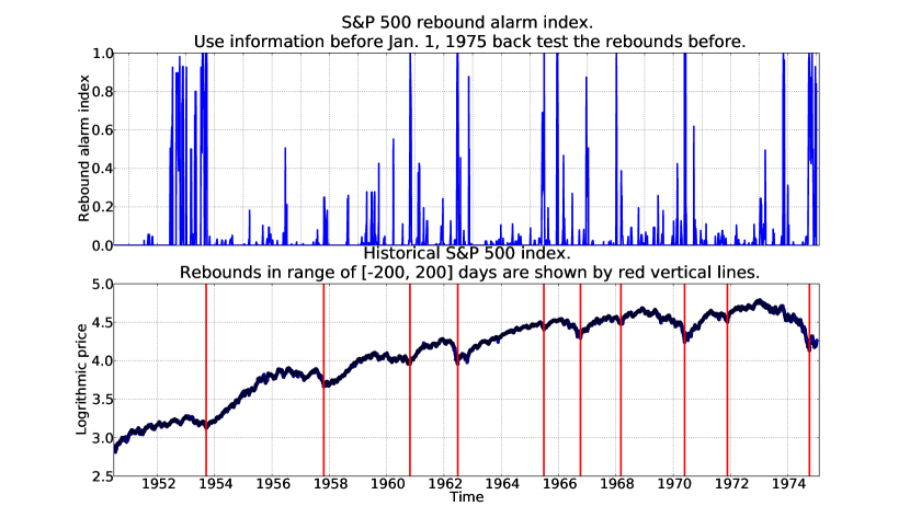
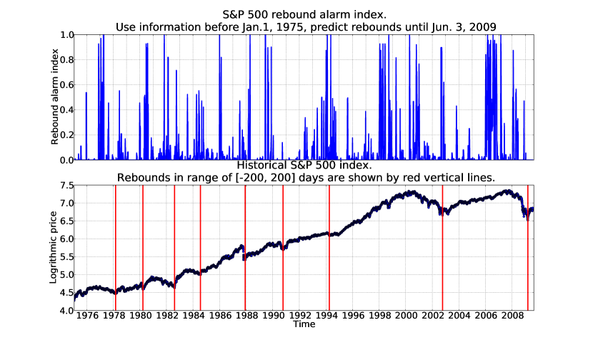
Using this technique, the prediction day $t_{2}$ is scanned from 1975-01-01 until 2009-07-22 in steps of 50 days. We then construct the time series of the rebound alarm index over this period and with this resolution of 50 days. The comparison of this rebound alarm index with the historical financial index (Figure 4) shows a good correlation, but there are also some false positive alarms (1977, 1998, 2006), as well as some false negative missed rebounds (1990). Many false positive alarms such as in 1998 and 2006 are actually associated with rebounds. But these rebounds have smaller amplitudes than our qualifying threshold targets. Concerning the false negative (missed rebound) in 1990, the explanation is probably that the historical prices preceeding this rebound does not follow the JLS model specification. Rebounds may result from several mechanisms and the JLS model only provides one of them, arguably the most important. Overall, the predictability of the rebound alarm index shown in Figure 4, as well as the relative cost of the two types of errors (false positives and false negatives) can be quantified systematically, as explained in the following sections. The major conclusion is that the rebound alarm index has a prediction skill much better than luck, as quantified by error diagrams.

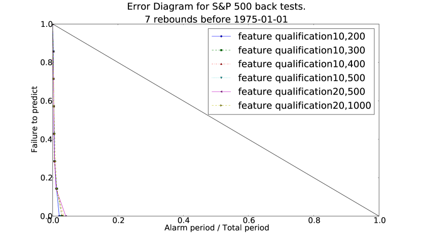
IV.3 Error Diagram

We have qualitatively seen that the feature qualifications method using back testing and forward prediction can generate a rebound alarm index that seems to detect and predict well observed rebounds in the S&P 500 index. We now quantify the quality of these predictions with the use of error diagrams Mochan (1997); Mochan and Kagan (1992). We create an error diagram for predictions after 1975-01-01 with a certain feature qualification in the following way:

1. Count the number of rebounds after 1975-01-01 as defined in section III.2 and expression (16). There are 9 rebounds.

2. Take the rebound alarm index time series (after 1975-01-01) and sort the set of all alarm index values in decreasing order. There are 12,600 points in this series and the sorting operation delivers a list of 12,600 index values, from the largest to the smallest one.

3. The largest value of this sorted series defines the first threshold.

4. Using this threshold, we declare that an alarm starts on the first day that the unsorted rebound alarm index time series exceeds this threshold. The duration of this alarm $D_{a}$ is set to 41 days, since the longest distance between a rebound and the day with index greater than the threshold is 20 days. Then, a prediction is deemed successful when a rebound falls inside that window of 41 days.

5. If there are no successful predictions at this threshold, move the threshold down to the next value in the sorted series of alarm index.

6. Once a rebound is predicted with a new value of the threshold, count the ratio of unpredicted rebounds (unpredicted rebounds / total rebounds in set) and the ratio of alarms used (duration of alarm period / 12,600 prediction days). Mark this as a single point in the error diagram.

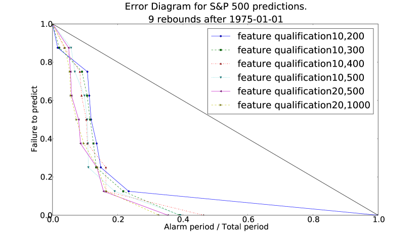
In this way, we will mark 9 points in the error diagram for the 9 rebounds.

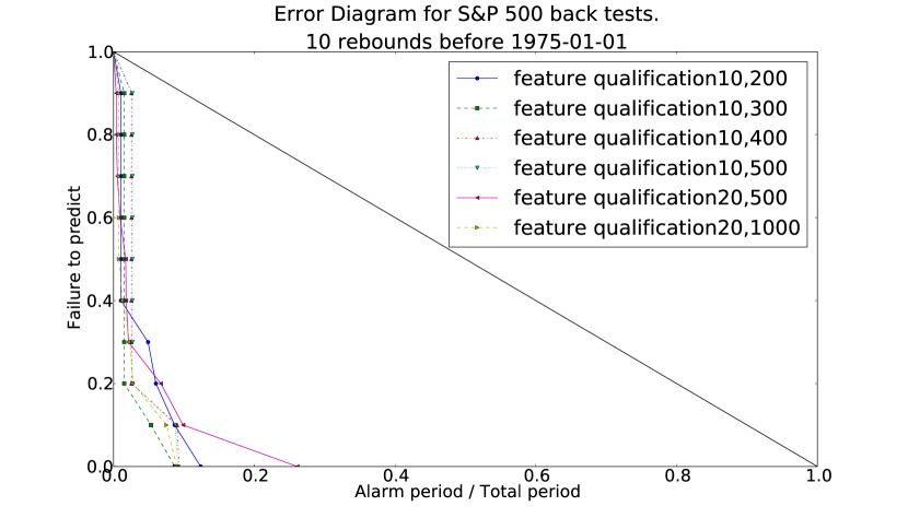
The aim of using such an error diagram in general is to show that a given prediction scheme performs better than random. A random prediction follows the line $y=1-x$ in the error diagram. A set of points below this line indicates that the prediction is better than randomly choosing alarms. The prediction is seen to improve as more error diagram points are found near the origin (0, 0). The advantage of error diagrams is to avoid discussing how different observers would rate the quality of predictions in terms of the relative importance of avoiding the occurrence of false positive alarms and of false negative missed rebounds. By presenting the full error diagram, we thus sample all possible preferences and the unique criterion is that the error diagram curve be shown to be statistically significantly below the anti-diagonal $y=1-x$.

In Figure 5, we show error diagrams for different feature qualification pairs $(\alpha,\beta)$. Note the 9 points representing the 9 rebounds in the prediction set. We also plot the 11 points of the error diagrams for the learning set in Figure 6.

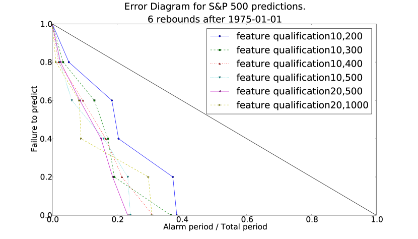
As a different test of the quality of this pattern recognition procedure, we repeated the entire process but with a rebound now defined as the minimum price within a window of $2\times 365$ days instead of $2\times 200$ days, as before. These results are shown in Figures 7-8.

IV.4 Bayesian inference

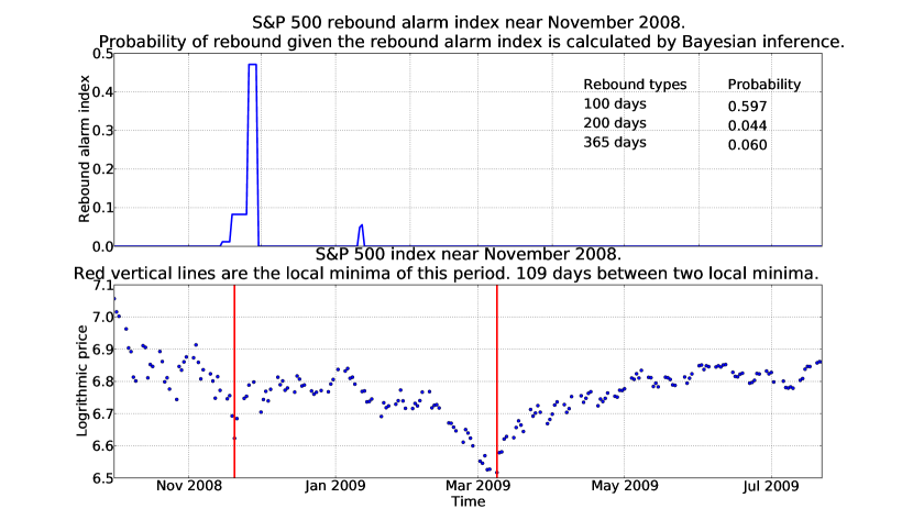
Given a value of the predictive rebound alarm index, we can also use the historical rebound alarm index combined with Bayesian inference to calculate the probability that this value of the rebound alarm index will actually be followed by a rebound. We use predictions near the end of November, 2008 as an example. From Figure 4, we can see there is a strong rebound signal in that period. We determine if this is a true rebound signal by the following method:

1. Find the highest rebound alarm index $Lv$ around the end of November 2008.

2. Calculate $D_{total}$, the number of days in the interval from 1975-01-01 until the end of the prediction set, 2009-07-22.

3. Calculate $D_{Lv}$, the number of days which have a rebound alarm index greater than or equal to $Lv$.

4. The probability that the rebound alarm index is higher than $Lv$ is estimated by

   $$P(RI\geq Lv)=\frac{D_{Lv}}{D_{total}}$$ (31)

5. The probability of a day being near the bottom of a rebound is estimated as the number of days near real rebounds over the total number of days in the predicting set:

   $$P(rebound)=\frac{D_{rw}N_{rebound}}{D_{total}},$$ (32)

   where $N_{rebound}$ is the number of rebounds we can detect after 1975-01-01 and $D_{rw}$ is the rebound width, i.e. the number of days near the real rebound in which we can say that this is a successful prediction. For example, if we say that the prediction is good when the predicted rebound time and real rebound time are within 10 days of each other, then the rebound width $D_{rw}=10\times 2+1=21$.

6. The probability that the neighbor of a rebound has a rebound alarm index larger than $Lv$ is estimated as

   $$P(RI\geq Lv|rebound)=\frac{N_{0}}{N_{rebound}}$$ (33)

   where $N_{0}$ is the number of rebounds in which

   $$\sup_{|d-rebound|\leq 20}RI_{d}\geq Lv.$$ (34)

7. Given that the rebound alarm index is higher than $Lv$, the probability that the rebound will happen in this period is given by Bayesian inference:

   $$P(rebound|RI\geq Lv)=\frac{P(rebound)\times P(RI\geq Lv|rebound)}{P(RI\geq Lv)}$$ (35)

Averaging $P(rebound|RI\geq Lv)$ for all the different feature qualifications gives the probability that the end of November 2008 is a rebound as 0.044. By comparing with observations, we see that this period is not a rebound. We obtain a similar result by increasing the definition of rebound from 200 days before and after a local minimum to 365 days, yielding a probability of 0.060.

When we decrease the definition to 100 days, the probability that this period is a rebound jumps to 0.597. The reason for this sudden jump is shown in Figure 9 where we see the index around this period and the S&P 500 index value. From the figure, we find that this period is a local minimum within 100 days, not more. This is consistent with what Bayesian inference tells us. However, we have to address that the more obvious rebound in March 2009 is missing in our rebound alarm index. Technically, one can easily find that this is because the end of crash is not consistent with the beginning of rebound in this special period.

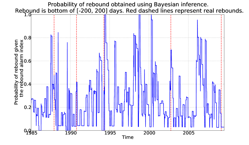
In this case, we then test all the days after 1985-01-01 systematically by Bayesian inference using only prediction data (rebound alarm index) after 1975-01-01. To show that the probability that $RI\geq Lv$ is stable, we cannot start Bayesian inference too close to the initial predictions so we choose 1985-01-01 as the beginning time. We have 5 ‘bottoms’ (troughs) after this date, using the definition of a minimum within $\pm 200$ days.

For a given day $d$ after 1985-01-01, we know all values of the rebound alarm index from 1975-01-01 to that day. Then we use this index and historical data of the asset price time series in this time range to calculate the probability that $d$ is the bottom of the trough, given that the rebound alarm index is larger than $Lv$, where $Lv$ is defined as

$$Lv=\sup_{d-t<50}RI_{t}$$ (36)

To simplify the test, we only consider the case of feature qualification pair (10, 200), meaning that the trait is a feature of Class I only if it shows in Class I more than 10 times and in Class II less than 200 times. Figure 10 shows that the actual rebounds occur near the local highest probability of rebound calculated by Bayesian inference. This figure also illustrates the existence of false positive alarms, i.e., large peaks of the probability not associated with rebounds that we have characterized unambiguously at the time scale of $\pm 200$ days.

V Trading strategy

In order to determine if the predictive power of our method provides a genuine and useful information gain, it is necessary to estimate the excess return it could generate. The excess return is the real return minus the risk free rate transformed from annualized to the duration of this period. The annualized 3-month US treasury bill rate is used as the risk free rate in this paper. We thus develop a trading strategy based on the rebound alarm index as follows. When the rebound alarm index rises higher than a threshold value $Th$, then with a lag of $Os$ days, we buy the asset. This entry strategy is complemented by the following exit strategy. When the rebound alarm index goes below $Th$, we still hold the stock for another $Hp$ days, with one exception. Consider the case that the rebound alarm index goes below $Th$ at time $t_{1}$ and then rises above $Th$ again at time $t_{2}$. If $t_{2}-t_{1}$ is smaller than the holding period $Hp$, then we continue to hold the stock until the next time when the rebound alarm index remains below $Th$ for $Hp$ days.

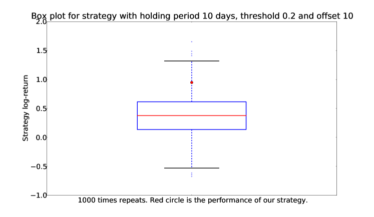
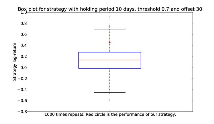
The performance of this strategy for some fixed values of the parameters is compared with random strategies, which share all the properties except for the timing of entries and exits determined by the rebound alarm index and the above rules. The random strategies consist in buying and selling at random times, with the constraint that the total holding period (sum of the holding days over all trades in a given strategy) is the same as in the realized strategy that we test. Implementing 1000 times these constrained random strategies with different random number realizations provide the confidence intervals to assess whether the performance of our strategy can be attributed to real skill or just to luck.

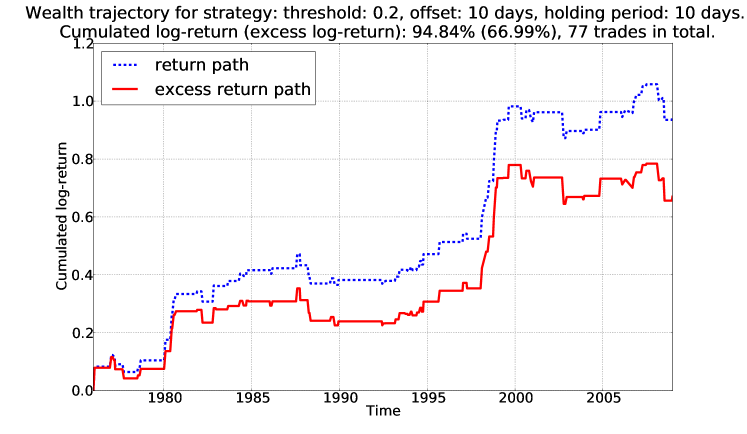
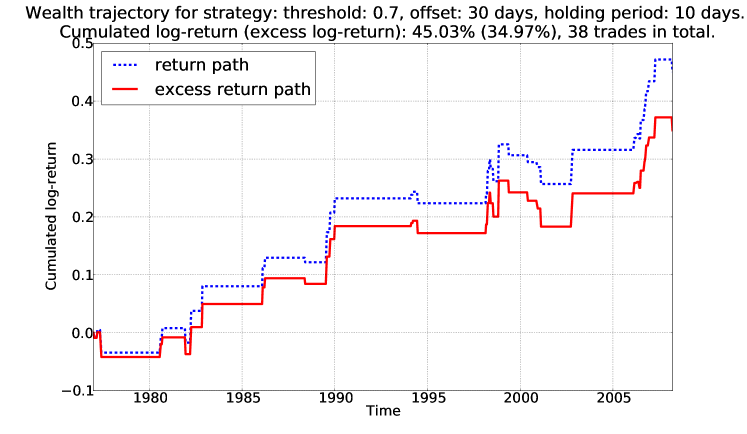
Results of this comparison are shown in Table 3 for two sets of parameter values. The p-value is a measure of the strategies’ performance, calculated as the fraction of corresponding random strategies that are better than or equal to our strategies. The lower the p-value is, the better the strategy is compared to the random portfolios. We see that all of our strategies’ cumulative excess returns are among the top 5-6% out of 1000 corresponding random strategies’ cumulative excess returns. Box plots for each of the strategies are also presented in Figures 11-12.

The cumulative returns as well as the cumulative excess returns obtained with the two strategies as a function of time are shown in Figures 13-14. These results suggest that these two strategies would provide significant positive excess return. Of course, the performance obtained here are smaller than the naive buy-and-hold strategy, consisting in buying at the beginning of the period and just holding the position. The comparison with the buy-and-hold strategy would be however unfair as our strategy is quite seldom invested in the market. Our goal here is not to do better than any other strategy but to determine the statistical significance of a specific signal. For this, the correct method is to compare with random strategies that are invested in the market the same fraction of time. It is obvious that we could improve the performance of our strategy by combining the alarm indexes of bubbles and of negative bubbles, for instance, but this is not the goal here.

We also provide the Sharpe ratio as a measure of the excess return (or risk premium) per unit of risk. We define it per trade as follows

$$S=\frac{E[R-R_{f}]}{\sigma}$$ (37)

where $R$ is the return of a trade, $R_{f}$ is the risk free rate (we use the 3-month US treasury bill rate) transformed from annualized to the duration of this trade given in Table 3 and $\sigma$ is the standard deviation of the returns per trade. The higher the Sharpe ratio is, the higher the excess return under the same risk.

The bias ratio is defined as the number of trades with a positive return within one standard deviation divided by one plus the number of trades which have a negative return within one standard deviation:

$$BR=\frac{\#\{r|r\in[0,\sigma]\}}{1+\#\{r|r\in[-\sigma,0)\}}$$ (38)

In Eq. (38), $r$ is the excess return of a trade and $\sigma$ is the standard deviation of the excess returns. This ratio detects valuation bias.

To see the performance of our strategies, we also check all the possible random trades with a holding period equals to the average duration of our strategies, namely 25 days and 17 days for strategy I and II respectively. The average Sharpe and bias ratios of these random trades are shown in Table 3. Both Sharpe and bias ratios of our strategies are greater than those of the random trades, confirming that our strategies deliver a larger excess return with a stronger asymmetry towards positive versus negative returns.

As another test, we select randomly the same number of random trades as in our strategies, making sure that there is no overlap between the selected trades. We calculate the Sharpe and bias ratios for these random trades. Repeating this random comparative selection 1000 times provides us with p-values for the Sharpe ratio and for bias ratio of our strategies. The results are presented in Table 3. All the p-values are found quite small, confirming that our strategies perform well.

VI Conclusion

We have developed a systematic method to detect rebounds in financial markets using “negative bubbles,” defined as the symmetric of bubbles with respect to a horizontal line, i.e., downward accelerated price drops. The aggregation of thousands of calibrations in running windows of the negative bubble model on financial data has been performed using a general pattern recognition method, leading to the calculation of a rebound alarm index. Performance metrics have been presented in the form of error diagrams, of Bayesian inference to determine the probability of rebounds and of trading strategies derived from the rebound alarm index dynamics. These different measures suggest that the rebound alarm index provides genuine information and suggest predictive ability. The implemented trading strategies outperform randomly chosen portfolios constructed with the same statistical characteristics. This suggests that financial markets may be characterized by transient positive feedbacks leading to accelerated drawdowns, which develop similarly to but as mirror images of upward accelerating bubbles. Our key result is that these negative bubbles have been shown to be predictably associated with large rebounds or rallies.

In summary, we have expanded the evidence for the possibility to diagnose bubbles before they terminate Sornette et al. (2010b), by adding the phenomenology and modeling of “negative bubbles” and their anticipatory relationship with rebounds. The present paper contributes to improving our understanding of the most dramatic anomalies exhibited by financial markets in the form of extraordinary deviations from fundamental prices (both upward and downward) and of extreme crashes and rallies. Our results suggest a common underlying origin to both positive and negative bubbles in the form of transient positive feedbacks leading to identifiable and reproducible faster-than-exponential price signatures.

VII List of Symbols

Table 1: List of symbols

$h(t)$	hazard rate
$p(t)$	stock price
$A,B,C$	linear parameters of the JLS model
$t_{c}$	critical time in the JLS model at which the bubble ends
$m$	exponent parameter in the JLS model
$\omega$	frequency parameter in the JLS model
$\phi$	phase parameter in the JLS model
$b$	parameter controlling the positivity of the hazard rate in the JLS model
$Rbd$	rebound time
$C_{I}$	set of Class I fits
$C_{II}$	set of Class II fits
$G_{i}$	set of Group i fits
$IP$	informative parameter
$A$	questionnaire
$\tau$	trait
$(\alpha,\beta)$	feature qualification pair
$RI$	rebound alarm index
$Lv$	highest rebound alarm index around a certain time
$Th$	threshold value for the trading strategy
$Os$	offset for the trading strategy
$Hp$	holding period for the trading strategy
$S$	Sharpe ratio
$R_{f}$	risk free rate
$r,R-R_{f}$	excess return of a trade
$BR$	bias ratio
$\#$	number of a set

Table 2: Traits for series A = (0,1,-1,-1)

p	q	r	(P,Q,R)
1	1	1	0
1	2	2	0,1
1	2	3	0,1,-1
1	2	4	0,1,-1
1	3	3	0,-1
1	3	4	0,-1,-1
1	4	4	0,-1
2	2	2	1
2	3	3	1,-1
2	3	4	1,-1,-1
2	4	4	1,-1
3	3	3	-1
3	4	4	-1,-1
4	4	4	-1

Table 3: Performances of two strategies: Strategy I ($Th=0.2,Os=10,Hp=10$) and Strategy II ($Th=0.7,Os=30,Hp=10$).

	Strategy I	Strategy II
Threshold  $Th$	0.2	0.7
Offset  $Os$	10	30
Holding period  $Hp$	10	10
Number of trades	77	38
Success rate
(fraction of trades with positive return)	66.2%	65.8%
Total holding days	1894 days	656 days
Fraction of time when invested	15.0%	5.2%
Cumulated log-return	95%	45%
cumulated excess log-return	67%	35%
Average return per trade	1.23%	1.19%
Average trade duration	24.60 days	17.26 days
$p$-value of cumulative excess return	0.055	0.058
Sharpe ratio per trade	0.247	0.359
Sharpe ratio of random trades
(holding period equals average trade duration)	0.025	0.021
$p$-value of Sharpe ratio	0.043	0.036
Bias ratio	1.70	1.36
Bias ratio of random trades
(holding period equals average trade duration)	1.27	1.25
$p$-value of bias ratio	0.105	0.309

References

Figure 1: Upper panel: Significant drawdown of nearly $50\%$ from 1973-01-01 to 1974-10-01 (time window delineated by the two black dashed vertical lines) with very clear log-periodic oscillations, followed by a strong positive rebound. The best fits from taboo search are used to form a 90% confidence interval for the critical time $t_{c}$ shown by the light shadow area. The dark shadow area corresponds to the 20-80 quantiles region of the predicted rebounds. Lower panel: the same phenomenon is observed in foreign exchange market. The plot shows the fitted results for USD/EUR change rate from 2006-07-01 to 2008-04-01. The USD/EUR change rate performed a significant drawdown with very clear log-periodic oscillations, followed by a strong positive rebound.

Figure 2: (upper) Histogram of the critical times $t_{c}$ over the set of 2,568 time intervals for which negative bubbles are detected by the condition that the fits of $\ln p(t)$ by expression (8) satisfy condition (11). (lower) Plot of $-\ln p(t)$ versus time for the S&P 500 index. Note that peaks in this figure correspond to valleys in actual price.

Figure 3: Rebound alarm index and log-price of the S&P 500 Index for the learning set, where $t_{2}$ and $t_{c}$ are both before Jan. 1, 1975. (upper) Rebound alarm index for the learning set using feature qualification pair $(10,200)$. The rebound alarm index is in the range $[0,1]$. The higher the rebound alarm index, the more likely is the occurrence of a rebound. (lower) Plot of $\ln p(t)$ versus time of S&P Index. Red vertical lines indicate rebounds defined by local minima within plus and minus 200 days around them. Note that these rebounds are the historical “change of regime” rather than only the jump-like reversals. The jump-like reversals, 1972, 1974 as examples, are included in these rebounds. They are located near clusters of high values of the rebound alarm index of the upper figure.

Figure 4: Rebound alarm index and log-price of S&P 500 Index for the predicting set after Jan. 1, 1975. (upper) Rebound alarm index for predicting set using feature qualification pair $(10,200)$. The rebound alarm index is in the range [0,1]. The higher the rebound alarm index, the more likely is the occurrence of a rebound. (lower) Plot of $\ln p(t)$ versus time of the S&P Index. Red vertical lines indicate rebounds defined by local minima within in plus and minus 200 days. They are located near clusters of high values of the rebound alarm index of the upper figure.

Figure 5: Error diagram for predictions after Jan. 1, 1975 with different types of feature qualifications. Feature qualification $\alpha,\beta$ means that, if the occurrence of a certain trait in Class I is larger than $\alpha$ and less than $\beta$, then we call this trait a feature of Class I and vice versa. See text for more information.

Figure 6: Same as Figure 5 but for the learning set before Jan. 1, 1975.

Figure 7: Same as Figure 5 but with the different definition of a rebound determined as the day with the smallest price within the 365 days before it and the 365 days after it.

Figure 8: Same as Figure 7 for the learning set before Jan. 1, 1975.

Figure 9: Rebound alarm index and market price near and after November 2008.

Figure 10: Probability of rebound as a function of time $t$, given the value of the rebound alarm index at $t$, derived by Bayesian inference applied to bottoms at the time scale of $\pm 200$ days. The feature qualification is (10, 200). $Lv$ is the largest rebound index in the past 50 days. The vertical red lines show the locations of the realized rebounds in the history of the S&P500 index.

Figure 11: Box plot for Strategy I ($Th=0.2,Os=10,Hp=10$). Lower and upper horizontal edges (blue lines) of box represent the first and third quartiles. The red line in the middle is the median. The lower and upper black lines are the 1.5 interquartile range away from quartiles. Points between quartiles and black lines are outliers and points out of black lines are extreme outliers. Our strategy return is marked by the red circle. This shows our strategy is an outlier among the set of random strategies. The log-return ranked 55 out of 1000 random strategies.

Figure 12: Same as figure 11 for Strategy II ($Th=0.7,Os=30,Hp=10$). The log-return ranked 58 out of 1000 random strategies.

Figure 13: Wealth trajectory for Strategy I ($Th=0.2,Os=10,Hp=10$). Major performance parameters of this strategy are: 77 trading times; 66.2% trades have positive return; 1894 total holding days, which is 15.0% of total time. Accumulated log-return is 95% and average return per trade is 1.23%. Average trade length is 24.60 days. P-value of this strategy is 0.055

Figure 14: Wealth trajectory for Strategy II ($Th=0.7,Os=30,Hp=10$). Major performance parameters of this strategy are: 38 trading times; 65.8% trades have positive return; 656 total holding days, which is 5.2% of total time. Accumulated log-return is 45% and average return per trade is 1.19%. Average trade length is 17.26 days. P-value of this strategy is 0.058

References

- Abreu and Brunnermeier (2003) Abreu, D., Brunnermeier, M. K., 2003. Bubbles and crashes. Econometrica 71(1), 173–204.
- Barberis et al. (1998) Barberis, N., Shleifer, A., Vishny, R., 1998. A model of investor sentiment. Journal of Financial Economics 49(3), 307–343.
- Blanchard and Watson (1982) Blanchard, O., Watson, M., 1982. Bubbles, rational expectations and speculative markets. in: Wachtel, P. ,eds., Crisis in Economic and Financial Structure: Bubbles, Bursts, and Shocks. Lexington Books: Lexington.
- Bondt and Thaler (1985) Bondt, W. M. D., Thaler, R., 1985. Does the stock market overreact? Journal of Finance 40, 793–805.
- Campbell and Shiller (1988) Campbell, J. Y., Shiller, R. J., 1988. The dividend-price ratio and expectations of future dividends and discount factors. Review of Financial Studies 1(3), 195–228.
- Chakravarti et al. (1967) Chakravarti, I., Roy, J., Laha, R., 1967. Handbook of methods of applied statistics. John Wiley and Sons 1, 392–394.
- Chen et al. (2002) Chen, J., Hong, H., Stein, J. C., 2002. Breadth of ownership and stock returns. Journal of Financial Economics 66, 171–205.
- Cvijovic and Klinowski (1995) Cvijovic, D., Klinowski, J., 1995. Taboo search: an approach to the multiple minima problem. Science 267 (5188), 664–666.
- Daniel et al. (1998) Daniel, K., Hirshleifer, D., Subrahmanyam, A., 1998. Investor psychology and security market underand overreactions. Journal of Finance 53, 1839–1885.
- DeLong et al. (1990) DeLong, J. B., Shleifer, A., Summers, L. H., Waldmann, R. J., 1990. Noise trader risk in financial markets. Journal of Political Economy 98(4), 703–738.
- Duffie et al. (2002) Duffie, D., Garleanu, N., Pedersen, L. H., 2002. Securities lending, shorting, and pricing. Journal of Financial Economics 66, 307–339.
- Galbraith (1997) Galbraith, J., 1997. The great crash, 1929. Boston : Houghton Mifflin Co.
- Gelfand et al. (1976) Gelfand, I., Guberman, S., Keilis-Borok, V., Knopoff, L., Press, F., E.Ya.Ranzman, Rotwain, I., Sadovsky, A., 1976. Pattern recognition applied to earthquake epicenters in california. Physics of The Earth and Planetary Interiors 11 (3), 227–283.
- Gluzman and Sornette (2002) Gluzman, S., Sornette, D., 2002. Classification of possible finite-time singularities by functional renormalization. Physical Review E 6601, 016134.
- Goriely and Hyde (2000) Goriely, A., Hyde, C., 2000. Necessary and sufficient conditions for finite time singularities in ordinary differential equations. Journal of Differential equations 161, 422–448.
- Gurkaynak (2008) Gurkaynak, R., 2008. Econometric tests of asset price bubbles: Taking stock. Journal of Economic Surveys 22 (1), 166–186.
- Harrison and Kreps (1978) Harrison, M., Kreps, D., 1978. Speculative investor behavior in a stock market with heterogeneous expectations. Quarterly Journal of Economics 92, 323–336.
- Hong et al. (2005) Hong, H., Kubik, J. D., Stein, J. C., 2005. Thy neighbor’s portfolio: Word-of-mouth effects in the holdings and trades of money managers. Journal of Finance 60, 2801–2824.
- Ide and Sornette (2002) Ide, K., Sornette, D., 2002. Oscillatory finite-time singularities in finance, population and rupture. Physica A 307, 63–106.
- Jarrow (1980) Jarrow, R., 1980. Heterogeneous expectations, restrictions on short sales, and equilibrium asset prices. Journal of Finance 35, 1105–1113.
- Jegadeesh and Titman (1993) Jegadeesh, N., Titman, S., 1993. Returns to buying winners and selling losers: Implications for stock market effciency. Journal of Finance 48(1), 65–91.
- Jegadeesh and Titman (2001) Jegadeesh, N., Titman, S., 2001. Profitability of momentum strategies: An evaluation of alternative explanations. Journal of Finance 54, 699–720.
- Jiang et al. (2010) Jiang, Z.-Q., Zhou, W.-X., Sornette, D., Woodard, R., Bastiaensen, K., Cauwels, P., 2010. Bubble diagnosis and prediction of the 2005-2007 and 2008-2009 chinese stock market bubbles. Journal of Economic Behavior and Organization 74, 149–162.
- Johansen et al. (2000) Johansen, A., Ledoit, O., Sornette, D., 2000. Crashes as critical points. International Journal of Theoretical and Applied Finance 3 (2), 219–255.
- Johansen and Sornette (1999) Johansen, A., Sornette, D., 1999. Critical crashes. Risk 12 (1), 91–94.
- Johansen and Sornette (2001a) Johansen, A., Sornette, D., 2001a. Finite-time singularity in the dynamics of the world population and economic indices. Physica A 294 (3-4), 465–502.
- Johansen and Sornette (2001b) Johansen, A., Sornette, D., 2001b. Large stock market price drawdowns are outliers. Journal of Risk 4(2), 69–110.
- Johansen and Sornette (2006) Johansen, A., Sornette, D., 2006. Shocks, crashes and bubbles in financial markets. Brussels Economic Review (Cahiers economiques de Bruxelles) Special Issue on Nonlinear Analysis 49 (3/4).
- Johansen et al. (1999) Johansen, A., Sornette, D., Ledoit, O., 1999. Predicting financial crashes using discrete scale invariance. Journal of Risk 1 (4), 5–32.
- Kindleberger (2000) Kindleberger, C., 2000. Manias, panics, and crashes: a history of financial crises. 4th ed. New York: Wiley.
- Levenberg (1944) Levenberg, K., 1944. A method for the solution of certain non-linear problems in least squares. Quarterly of Applied Mathematics II 2, 164–168.
- Lintner (1969) Lintner, J., 1969. The aggregation of investors’ diverse judgments and preferences in purely competitive security markets. Journal of Financial and Quantitative Analysis 4, 347–400.
- Lux and Sornette (2002) Lux, T., Sornette, D., 2002. On rational bubbles and fat tails. Journal of Money, Credit and Banking 34 (3), 589–610.
- Marquardt (1963) Marquardt, D. W., 1963. An algorithm for least-squares estimation of nonlinear parameters. Journal of the Society for Industrial and Applied Mathematics 11 (2), 431–441.
- Miller (1977) Miller, E., 1977. Risk, uncertainty and divergence of opinion. Journal of Finance 32, 1151–1168.
- Mochan (1997) Mochan, G. M., 1997. Earthquake prediction as a decision making problem. Pure and Applied Geophysics 149, 233–247.
- Mochan and Kagan (1992) Mochan, G. M., Kagan, Y. Y., 1992. Earthquake prediction and its optimization. Journal of Geophysical Research 97, 4823–4838.
- Nagel (2010) Nagel, S., 2010. Evaporating liquidity. Stanford University Working Paper.
- Pedersen (2009) Pedersen, L. H., 2009. When everyone runs for the exit. International Journal of Central Banking 5(4), 177–199.
- Sammis and Sornette (2002) Sammis, S., Sornette, D., 2002. Positive feedback, memory and the predictability of earthquakes. Proceedings of the National Academy of Sciences USA 99 (SUPP1), 2501–2508.
- Scheinkman and Xiong (2003) Scheinkman, J., Xiong, W., 2003. Overconfidence and speculative bubbles. Journal of Political Economy 111, 1183–1219.
- Sornette (1998) Sornette, D., 1998. Discrete scale invariance and complex dimensions. Physics Reports 297 (5), 239–270.
- Sornette (2003) Sornette, D., 2003. Why stock markets crash (critical events in complex financial systems). Princeton University Press.
- Sornette and Johansen (1997) Sornette, D., Johansen, A., 1997. Large financial crashes. Physica A 245 N3-4, 411–422.
- Sornette et al. (2003) Sornette, D., Takayasu, H., Zhou, W.-X., 2003. Finite-time singularity signature of hyperinflation. Physica A 325, 492–506.
- Sornette et al. (2010a) Sornette, D., Woodard, R., Fedorovsky, M., Reimann, S., Woodard, H., Zhou, W.-X., 2010a. The financial bubble experiment: advanced diagnostics and forecasts of bubble terminations (the financial crisis observatory).
- Sornette et al. (2010b) Sornette, D., Woodard, R., Fedorovsky, M., Reimann, S., Woodard, H., Zhou, W.-X., 2010b. The financial bubble experiment: Advanced diagnostics and forecasts of bubble terminations volume ii–master document. http://arxiv.org/abs/1005.5675.
- v. Bothmer and Meister (2003) v. Bothmer, H.-C. G., Meister, C., 2003. Predicting critical crashes? a new restriction for the free variables. Physica A 320C, 539–547.
- Worton (1989) Worton, B., 1989. Kernel methods for estimating the utilization distribution in home-range studies. Ecology 70 (1), 164–168.