Finite temperature ordering of dilute graphene antiferromagnets

Abstract

We employ large-scale quantum Monte Carlo simulations to study the magnetic ordering transition among dilute magnetic moments randomly localized on the graphene honeycomb lattice, induced by long-ranged RKKY interactions at low charge carrier concentration. In this regime the effective exchange interactions are ferromagnetic within each sublattice, and antiferromagnetic between opposite sublattices, with an overall cubic decay of the interaction strength with the separation between the moments. We verify explicitly, that this commensurability leads to antiferromagnetic order among the magnetic moments below a finite transition temperature in this two-dimensional system. Furthermore, the ordering temperature shows a crossover in its power-law scaling with the moments’ dilution from a low- to a high-concentration regime.

I Introduction

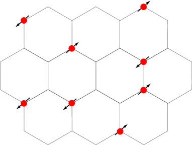
Since the discovery of the single-layer hexagonal carbon sheets of graphene, its fascinating physical properties have stimulated a lot of research on the static and transport properties of fermions on the two-dimensional hexagonal lattice geim07a ; castroneto09a . Soon after its discovery, the role of disorder effects on graphene has opened up new research horizons peres06 ; aleiner06 . In particular, disorder induced localized states pereira06 and magnetism vozmediano05 ; kumazaki07 ; uchoa08 ; palacios08 have attracted a lot of interest. For instance, it was found that graphene’s electronic properties give rise to the efficient formation of magnetic moments from adatoms located on the graphene surface uchoa08 , or simply from defects vozmediano05 ; kumazaki07 ; palacios08 . Motivated by such studies, we here consider a situation such as shown in Fig. 1, where local moments are induced in a graphene sheet by for instance adatoms or defects, each single magnetic moment being associated with a particular lattice site of the underlying lattice brey07 ; saremi07 . At low carrier concentration, the low density of states near the Dirac points suppresses the Kondo effect and allows for the formation of magnetically ordered states by the interaction between the localized moments and the conduction electrons brey07 ; saremi07 ; sengupta08 . Namely, they induce long-ranged Ruderman-Kittel-Kasuya-Yosida (RKKY) exchange interactions between the localized magnetic moments, described by the Hamiltonian

$${{H}}=\sum_{i,j}J_{ij}^{{\rm RKKY}}\>\mathbf{S}_{i}\cdot\mathbf{S}_{j}.$$ (1)

The effective interaction $J_{ij}^{{\rm RKKY}}$, mediated by itinerant electrons, strongly depends on the electronic properties at the Fermi energy. While in typical metals an oscillating coupling at $2k_{F}$ is expected ($k_{F}$ being the Fermi wave vector), decaying as $1/r^{2}$ in two dimensions ($r$ being the relative distance between impurities), the semi-metallic properties of graphene lead to a different behavior vozmediano05 ; brey07 ; saremi07 . Indeed, the absence of an extended Fermi surface leads to a cancellation of the $1/r^{2}$ term and leaves the next term decaying as $1/r^{3}$ without any $2k_{F}$ oscillations. Furthermore, it was revealed in Refs. brey07 ; saremi07 that pair-wise interactions are ferromagnetic (antiferromagnetic) among the same (different) sublattice on the bipartite honeycomb lattice of graphene.

Figure 1: (Color online) Magnetic moments localized on a honeycomb lattice. Due to the commensurate nature of the long-ranged exchange interaction, the moments order antiferromagnetically below a finite transition temperature.

This means for the exchange couplings in Eq. (1), that

$$J_{ij}^{{\rm RKKY}}=\epsilon_{ij}J({|\mathbf{r}_{i}-\mathbf{r}_{j}}|),\quad J(r)=\frac{J}{r^{3}},$$ (2)

with $J>0$ and $\epsilon_{ij}=-1$ $(+1)$ if $i$ and $j$ belong to the same (different) sublattice brey07 ; saremi07 . Here, $\mathbf{r}_{i}$ denotes the (random) position of the $i$-th magnetic moment $\mathbf{S}_{i}$ on the honeycomb lattice, which we consider to be spin-$\frac{1}{2}$ quantum spins, in order to explore the extreme quantum limit. Larger spin values of the moments will not qualitatively change the results. The commensurate nature of the RKKY interactions was linked to the bipartiteness of the underlying lattice geometry saremi07 . In a more recent work bunder09 , this general result was called into question for graphene nanoribbons, due to the presence of zero-mode contributions. In bulk graphene however, these corrections vanish in the thermodynamic limit bunder09 , thus recovering the commensurate form of the interactions in Eq. (2). In the following, we focus on the most basic model that contains the main features of such exchange interactions (i.e. their commensurate, long-ranged nature) between the magnetic moments, and leave for discussion at the end of the paper several aspects relevant to graphene, such as doping effects, a finite extension of the localized moments, and structural defects.

The remainder of this paper is organized as follows: In the following section, we review some general results concerning long-range order in low-dimensional systems. Then, we present our numerical approach in Sec. III. The results of our simulations are discussed in Sec. IV and Sec. V. Concluding remarks are made in Sec. VI, while an appendix provides details about the relevant length and energy scales on the diluted honeycomb lattice. In the appendix, we furthermore introduce the notion of an effective coordination number for diluted magnetic moments, that will be convenient for the discussion in Sec. V.

II long-range order in 2D

Starting from the effective exchange interactions of Eq. (2) in Eq. (1), we explore its consequences for the finite-temperature ordering transition between magnetic moments on the honeycomb lattice. The stability of long-range magnetic order in $d\leq 2$ systems with power-law decaying interactions has been the subject of a large number of theoretical studies in the past mermin66 ; fisher72 ; brezin76 ; cardy81 ; haldane88 ; shastry88 ; nakano94 ; nakano95 ; vassiliev01 ; bruno01 ; luijten02 ; yusuf04 ; laflorencie05 ; beach07 . Regarding the Heisenberg model with $1/r^{\alpha}$ interactions, the seminal paper of Mermin and Wagner mermin66 , proving the absence of finite-$T$ spontaneous order if $\alpha>d+2$, was recently reconsidered by Bruno bruno01 , who gave stronger conditions, notably on the appearance of ferromagnetism for oscillatory interactions. For instance, an interaction of the form $\cos(k_{0}r)/r^{\alpha}$ ($k_{0}\neq 0$) cannot lead to finite-temperature ferromagnetism if $\alpha>5/2$. For the case under study here, Bruno’s result implies the absence of finite-temperature antiferromagnetic order for $\alpha>2d$ which does not deviate from Mermin-Wagner’s results in $d=2$.

Early renormalization group calculations on classical O($n$) models with $1/r^{d+\sigma}$ couplings predicted fisher72 ; brezin76 a $\sigma$-dependent criticality with a finite ordering temperature for $\sigma<d$: $T_{c}\propto(d-\sigma)/(n-1)$ when $\sigma\to d$ brezin76 . For instance, while for $\sigma<d/2$ exponents take exact ”classical” values ($\eta=2-\sigma$, $\nu=1/\sigma$, $\gamma=1$), our case $\sigma=1$ lies on the boundary of this regime where logarithmic corrections are expected fisher72 . In particular, the correlation length exponent turns out to be $\nu=1^{+}$, which fulfills the Harris criterion harris74 ; vojta06 $\nu>2/d$. From such a statement we expect on general grounds that clean and disordered systems with power-law interactions display similar critical behaviors if $\sigma\leq 1$. We indeed find, that the model in Eq. (1) exhibits at finite temperature a phase transition to an antiferromagnetically ordered Néel state, both in case of a fully covered lattice and also for the case of diluted magnetic moments, with apparently similar critical exponents.

In the following, we analyze in detail the dependence of the ordering temperature on the concentration $p$ of the magnetic moments. While in the realistic parameter regime the magnetic moments will be dilute, i.e. $p\ll 1$, we consider for completeness the whole range up to (and including) the case of full coverage $p=1$, where a magnetic moment resides on every lattice site. For the full coverage case, we also performed simulations for an underlying square lattice, in order to explore more generally the magnetic ordering transition in quantum antiferromagnets with long-range interactions in two dimensions. While in previous works nakano94 ; nakano95 ; vassiliev01 , the case of solely ferromagnetic interactions on a square lattice geometry has been analyzed, the current case and the effects of dilution have not been considered thus far.

III Methods

Figure 2: (Color online) Temperature dependence of the staggered magnetization $m_{AF}$ for different system sizes $L=8,16,32,40,48,56$, and $64$ for the occupation density $p=1$ (full coverage). The inset shows the temperature dependence of the specific heat $C_{V}$ for system sizes $L=16,48$, and $64$. The dashed lines indicate the position of the transition temperature as estimated from a finite size scaling analysis of the Binder parameter.

For our study, we employed large-scale quantum Monte Carlo simulations based on the stochastic series expansion representation sandvik99b , with an improved diagonal update scheme adapted to systems with long-ranged interactions sandvik03 . In addition, we used Walker’s method of alias walker77 in order to speed up the algorithm fukui09 . We performed simulations on finite systems with $N_{l}=2L^{2}$ lattice sites and linear system sizes ranging up to $L=192$, depending on the concentration $p$ of the magnetic moments. For $p<1$, we performed statistical averages over independent realizations of the moments’ distribution in a canonical ensemble, such that no sample-to-sample fluctuations in the total number of moments $N=p\times N_{l}$ result. Typically, we performed disorder averages over several thousand realizations, and verified that the calculated observables followed Gaussian distributions, as expected. We always employed period boundary conditions, and used the minimum image convention for the $1/r^{3}$-decaying exchange constants. For each choice of $p$ and $L$, we measured the staggered magnetization, obtained using the standard operator

$$\mathbf{S}_{AF}=\frac{1}{N}\sum_{i}^{N}\epsilon_{i}\mathbf{S}_{i},$$ (3)

after performing the disorder averaging as

$$m_{AF}=\sqrt{[\langle\mathbf{S}_{AF}^{2}\rangle]_{av}}.$$ (4)

Here, $\epsilon_{i}=\pm 1$, depending on the sublattice to which spin $i$ belongs on the honeycomb lattice, $\langle...\rangle$ denotes the QMC statistical mechanics expectation value for each realization of disorder, and $[...]_{av}$ the final disorder averaging. We also calculated the Binder parameter

$$Q=[\langle\mathbf{S}_{AF}^{4}\rangle]_{av}/[\langle\mathbf{S}_{AF}^{2}\rangle]_{av}^{2}.$$ (5)

We then used a finite size scaling analysis to extract the critical temperature and exponents from the finite size data of $m_{AF}$ and $Q$. More details about the finite size scaling analysis are provided below.

Figure 3: (Color online) Data collapse of the Binder parameters for the full case $p=1$ in a finite size scaling analysis. Here, $t=(T-T_{N})/T_{N}$ denotes the reduced temperature. The inset shows the Binder parameters $Q$ for different system sizes in the vicinity of the consecutive crossing points.

IV Full coverage

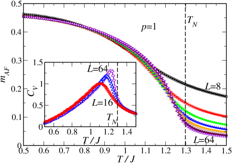
As a useful starting point in the absence of any disorder, we consider firstly the full coverage case $p=1$. In Fig. 2, we present the QMC data for the temperature dependence of the staggered magnetization for various system sizes. This data shows, that a finite temperature ordering transition takes place near $T\sim 1.3J$. This is also evident from the behavior of the specific heat $C_{V}$, shown in the inset of Fig. 2. It also exhibits pronounced finite size effects, that need to be accounted for in order to extract the transition temperature.

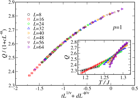
For this purpose, we calculated the Binder parameter $Q$ inside the transition region, for which the finite size data is shown in the inset of Fig. 3. The strongly moving crossing points in the data for consecutive system sizes again indicate significant finite size effects, that need to be taken into account in the further analysis. We thus employed a finite size scaling analysis including leading corrections to scaling beach05 , used in several precision studies on critical properties in quantum spin systems wang06 ; wenzel08a ; wenzel09a .

It is based on a scaling ansatz for the Binder parameter

$$Q(t,L)=(1+cL^{-\omega})g(tL^{1/\nu}+dL^{-\phi/\nu}),$$ (6)

with the reduced temperature $t=(T-T_{N})/T_{N}$, and the scaling function $g$. From this analysis, the critical exponent $\nu$ is also obtained. Furthermore, $\omega,\phi,c$, and $d$ describe the leading corrections to scaling, which are necessary in order to fit the QMC data obtained here for a system with long-ranged interactions on the limited system sizes available to our numerical study. Following Ref. wang06, , we represent $g$ up to forth-order in a Taylor expansion ($g(x)=g_{0}+g_{1}x+g_{2}x^{2}+g_{3}x^{3}+g_{4}x^{4}$), and use bootstrapping in combination with a standard Levenberg-Marquardt nonlinear optimization algorithm to perform the minimization procedure and fit the numerical data to the above scaling from.

In Fig. 3, we show the resulting data collapse for the case of $p=1$.

Figure 4: (Color online) Temperature dependence of the staggered magnetization $m_{AF}$ for different system sizes $L=32,64,96,128,160$, and $192$ for the occupation density $p=0.1$. The dashed line indicates the position of the transition temperature as estimated from a finite size scaling analysis of the Binder parameters.

We find that the QMC data can be fitted well to the above scaling form, leading to an estimate of the transition temperature of $T_{N}/J=1.298\pm 0.001$ with three significant digits. While the other fitting parameters are less constrained by the finite-size data (see below) – as observed also in the above-mentioned high-precision studies of short-range interacting quantum spin systems wang06 ; wenzel08a ; wenzel09a – we obtain from the finite-size analysis robust estimates of $T_{N}$, which is the quantity we are mainly interested in for this study; in particular, since we will analyse its dependence on the dilution $p$ in the following section. Furthermore, we obtain an estimate for the correlation length critical exponent $\nu=1.04\pm 0.02$. This value is in good agreement with the predicted value $\nu=1$ from the renormalization group approach fisher72 , the small deviations from this prediction being attributed to logarithmic corrections in the dependence of the correlation length on the reduced temperature fisher72 . However, given the restricted range of system sizes available to our QMC study, we are not in a position, to accurately account for these additional corrections. From the same finite-size data, we also obtain estimates for $\omega=0.4\pm 0.1$ and $\phi=0.6\pm 0.1$, which are less constrained within the bootstrapping analysis. Similar as for $\nu$, we expect residual finite-size effects also on these values due to the logarithmic corrections. These values are about a factor of two smaller than the values given e.g. in Ref. wang06, for the case of the quantum phase transition in bilayer Heisenberg models, where however the expected universality class is that of the three-dimensional Heisenberg transition instead of the mean-field behavior expected here. From the fitting procedure, we obtain non-zero values for both prefactors of the subleading finite-size corrections, $d=-2\pm 0.6$, and $c=-0.11\pm 0.06$. This exhibits the necessity of including the subleading finite-size corrections to the leading scaling behavior in Eq. (6). The Taylor expansion coefficients of the scaling function $g$ can be estimated from the bootstrapping analyis as $g_{0}=2.93\pm 0.04$, $g_{1}=0.18\pm 0.04$, $g_{2}=-0.1\pm 0.01$, $g_{3}=-0.001\pm 0.008$, $g_{4}=0.009\pm 0.003$. The last two coefficients remain more unconstrained than the other fitting parameters. This indicates that $g$ could also be represented well by a second order polynomial within the considered region close to $T_{N}$ with coefficients similar to those given above.

We performed an analysis for $p=1$ also for the case of an underlying square lattice, and obtained the transition temperature in that case to be $T_{N}/J=1.855\pm 0.02$, which is in fact close to the values obtained from QMC simulations and from using a Green’s function decoupling for the fully ferromagnetic case vassiliev01 ; nakano95 . Furthermore, for the square lattice, we obtain an estimate of $\nu=1.13\pm 0.07$, which within the error bars agrees with the result for the honeycomb lattice, but deviates more from the mean-field value. From the finite size scaling of $m_{AF}\propto L^{-\beta/\nu}$ at $T_{N}$, we extract the ratio $\beta/\nu=0.52\pm 0.04$, which within error bars agrees with the value $\beta/\nu=1/2$ from renormalization group calculations fisher72 . The estimates for $\omega=0.4\pm 0.1$ and $\phi=0.6\pm 0.1$, that we obtain for the square lattice, also agree within the error bars with the result for the honeycomb lattice. Again, this is expected, as the ordering transitions on both lattices belong to the same universality class.

V Randomly Diluted Moments

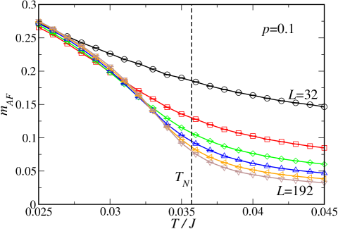
After having considered the full coverage limit, we now turn to the case of diluted magnetic moments, $p<1$. Also in this case we do obtain a finite temperature ordering transition. For example, the QMC data for the staggered magnetization at $p=0.1$ is shown in Fig. 4. The corresponding data for the Binder parameter is shown in the inset of Fig. 5.

Figure 5: (Color online) Data collapse of the Binder parameters for $p=0.1$ in a finite size scaling analysis. Here, $t=(T-T_{N})/T_{N}$ denotes the reduced temperature. The inset shows the Binder parameter $Q$ for different system sizes taken in the vicinity of the consecutive crossing points.

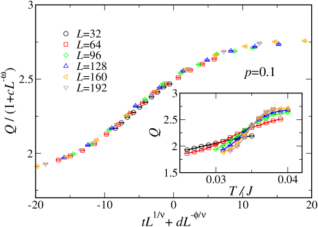
Performing the same finite size scaling analysis as before, we estimate the Néel temperature as $T_{N}/J=0.0357\pm 0.0006$ for $p=0.1$. The corresponding data collapse of the Binder parameter is shown in the main panel of Fig. 5. The estimate for the correlation length critial exponent $\nu=1.0\pm 0.02$ appears somewhat closer to the mean-field value, while the results for $\omega=0.4\pm 0.1$ and $\phi=0.6\pm 0.1$ agree well with the above values at $p=1$.

Proceeding in the same way for various values of $p$, we eventually obtain the dilution dependence of the Néel temperature shown in Fig. 6, which summarizes the main results from our numerical study. Concerning the estimates for the exponents $\nu$, $\omega$ and $\phi$, we cannot observe, within statistical errors, any systematic changes with $p$ from their values in the clean limit, which appears consistent with the discussion in Sec. II.

On the other hand, the transition temperature shows a strong dependence on $p$ that we now analyse further.

Figure 6: (Color online) Magnetic transition temperature $T_{N}$ as a function of the occupation density $p$. The inset shows the same data on a log-log plot. A power-law dependence proportional to $p^{3/2}$ for $p\lesssim 0.2$ is indicated by the dashed line.

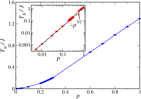
In the range $0.3\lesssim p<1$, this dependence is almost perfectly linear. An extrapolation of the linear suppression would exclude finite-temperature magnetic order below $p\sim 0.18$. However, we find the low-$p$ behavior of $T_{N}$ to deviate from this linear behavior. In fact, as seen from the inset of Fig. 6, which shows the same data on a log-log plot, below $p\sim 0.2$, $T_{N}$ exhibits an algebraic increase with $p$, scaling as

$$T_{N}\propto p^{3/2},\quad p\lesssim 0.2.$$ (7)

In the following, we discuss the relevant energy scales behind the different behavior of $T_{N}$ at high and low concentration of the magnetic moments:

On a two-dimensional lattice, dilute randomly distributed magnetic moments are separated by an average distance that scales as $\langle r\rangle\propto p^{-1/2}$ (on the honeycomb lattice $\langle r\rangle=p^{-1/2}/2$, cf. the appendix) which defines a typical coupling strength $J_{\rm typ}=J(\langle r\rangle)\propto p^{3/2}$. In the low-$p$ regime, we thus find that the Néel temperature scales with the characteristic energy scale set by $J_{\rm typ}$. At higher concentrations, the scaling of $T_{N}$ with $p$ becomes more mean-field-like, namely directly proportional to the mean-field average coupling (see Eq. (10) in the appendix) $J_{\rm avg}^{\rm MF}\propto p$. This leads to the linear behavior in $T_{N}$ observed at higher values of $p$. In this regime, the average nearest-neighbor distance between the magnetic moments is $\langle r\rangle\sim 1$, and does not vary much as a function of $p$. Its main effect is the reduction of exchange paths, as the number of bonds that each moment is associated with reduces linearly with $p$. The crossover results near $p\sim 0.25$, corresponding to a concentration regime beyond which the average distance becomes $\langle r\rangle\sim 1$, as shown in the appendix.

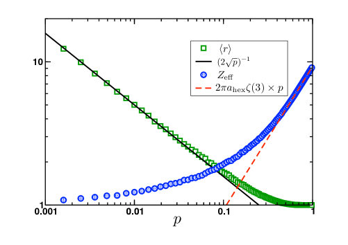
The behavior of $T_{N}$ can be qualitatively understood also with the help of a $p$-depended effective coordination number $Z_{\rm eff}(p)$, as defined in Eq. (11), which displays two distinct regimes: For large dilution $p\ll 1$ (i.e. for $\langle r\rangle\gg 1$), $Z_{\rm eff}\sim 1$, and the natural energy scale for the magnetic ordering is set by the coupling value at the average distance (i.e. $J_{\rm typ}$), because each moment has only a few neighbors to couple with and thus $T_{N}\sim J_{\rm typ}$. Increasing $p$, once $Z_{\rm eff}$ becomes significantly larger than one (i.e. once $\langle r\rangle\sim 1$) the relevant energy scale which controls the ordering of the moments will be controlled by the average $J_{\rm avg}^{\rm MF}$, directly proportional to $p$. As shown in the appendix, the crossover between these two regimes takes place near $p\sim 0.25$. It is interesting to compare such a concentration to the percolation threshold of the 2D honeycomb lattice $p^{*}\sim 0.697$ suding99 where nearest-neighbor interacting quantum spins lose long-range magnetic order in the ground state castro06 . The absence of any feature at $p^{*}$ in the present study is in fact consistent with the sizeable value of the effective coordination number $Z_{\rm eff}(p^{*})\sim 6.5$.

VI Discussion and conclusions

Motivated by recent results on the properties of RKKY interactions between localized magnetic moments on graphene brey07 ; saremi07 , we performed a systematic study of the finite-temperature ordering transition of dilute spin-1/2 magnetic moments on the honeycomb lattice, induced by a commensurate long-ranged exchange interaction. We found that in the low dilution regime, where the effective coordination number is close to unity (i.e. the average separation $\langle r\rangle\gg 1$), the Néel temperature scales with the typical coupling $J_{\rm typ}\propto p^{3/2}$. For larger occupations, the behavior crosses over to a mean-field-like linear reduction of the Néel temperature from its value in the full coverage case. We also presented estimates for the critical exponents $\beta$ and $\nu$, which within statistical errors are consistent with the prediction from previous renormalization group calculations for the ferromagnetic classical $O(3)$ model, given that additional logarithmic corrections are expected fisher72 . In our analysis, we considered the extreme quantum limit of $S=1/2$ magnetic moments. However, the physical picture will not change except that the Néel temperature will scale with $S(S+1)$ for higher quantum spins. For the future, it will be interesting to explore the critical properties of such diluted quantum magnets with long-ranged exchange interactions in more detail, also considering other decay rates of the exchange interactions. This would require the consideration of significantly larger lattices. Our main focus here was on the diluted case, relevant to the physical situation in graphene.

In the case of graphene, the RKKY coupling, controlled by the ratio between Coulomb repulsion $U$ and band-width $W$, is $J\sim U^{2}/W\sim 1$ eV vozmediano05 which for a moderate concentration $p\sim 10^{-2}$ would give a critical temperature $\sim 10$K. Of course this estimate is based on a very simple model of localized point-like magnetic impurities. A more realistic description should be able to incorporate (i) the spatial extension $\xi$ of the defects, (ii) the holes/electrons doping effects, (iii) lattice distortions (ripples for instance). Regarding (i), a finite area $\xi^{2}$ for a defect is expected to move the crossover concentration $p\sim 0.25$ above which MF behavior $T_{N}\sim p$ occurs towards a lower value $p\sim 0.25/\xi^{2}$. (ii) As already discussed in Ref. vozmediano05 , holes/electrons doping shifts the Fermi energy, thus leading to a finite Fermi wave vector $k_{F}\sim\sqrt{n_{c}}$ ($n_{c}$ being the carriers concentration). RKKY interactions will oscillate with a wave length $\lambda_{F}\sim 1/\sqrt{n_{c}}$, while the average distance between moments is $\langle r\rangle\sim 1/\sqrt{p}$. Therefore the above analysis, which ignores $2k_{F}$ oscillating terms is expected to be valid provided $n_{c}\ll p$. Alternatively, one expects the Néel order to be destroyed upon carrier doping in graphene sheets. For instance, using an electric field to control the Fermi level would render it possible to induce a transition from the Néel ordered regime for $k_{F}\ll\sqrt{p}$ onto a more complex regime at $k_{F}\sim\sqrt{p}$ where competing interactions, i.e. magnetic frustration, associated with random dilution are expected to provide all the ingredients to achieve spin-glass physics. We note that in the commensurate case at half-filling, the ferromagnetic and the antiferromagnetic exchange interactions actually have different prefactors saremi07 . However, this does not lead to any frustration, and hence including these prefactors will not destroy the finite temperature antiferromagnetic state. (iii) With respect to lattice distortions, it would be interesting to account for the characteristic ripples in the graphene structure geim07a ; castroneto09a and explore its consequences on the magnetic order, given the long-ranged nature of the exchange interactions. This would extend a recent study that considered this interplay between structural and magnetic properties within an effective Ising model with exponentially suppressed exchange interactions on the order of several lattice spacings rappoport09 .

Two directions appear feasible to experimentally probe for the two-dimensional magnetism in graphene at finite temperatures: using magnetic adatoms like Mn for instance, or extrinsic defects   that could be created by irradiation. In addition to randomly distributed moments, it will be interesting to explore the situation considered in Ref. uchoa08, , where the magnetic moments are placed using STM techniques onto specific lattice sites, and to examine the magnetic states induced by the RKKY interactions. For such studies, the effects of frustration could lead to exotic magnetic phases, the study of which is however beyond the scope of the quantum Monte Carlo approach, due to the infamous sign-problem troyer05a . In that respect, future experiments on graphene might even be employed as a quantum simulator for such magnetic clusters.

Appendix A Energy scales on the diluted honeycomb lattice

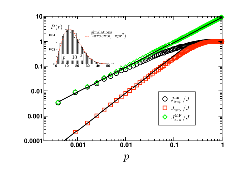
In order to gain insight into the role played by various energy scales, we performed a numerical analysis on a $L=5000$ diluted system, introducing a fraction $p$ of magnetic moments randomly on the honeycomb lattice. The nearest-neighbor distance (i.e. the distance from a randomly chosen moment to the closest other moment) obeys a probability distribution (see the inset of Fig. 7), that at low concentrations $p$ is very well described by

$$P(r)=2\pi rp\exp(-\pi pr^{2}),$$ (8)

thus resulting in an average nearest-neighbor distance $\langle r\rangle=p^{-1/2}/2$, shown in Fig. 8. This leads to a typical coupling strength $J_{\rm typ}=J(\langle r\rangle)\propto p^{3/2}$. It is interesting to compare this to the average nearest-neighbor coupling $J_{\rm avg}^{\rm nn}$, defined as

$$J_{\rm avg}^{\rm nn}=\int J(r)P(r){\rm d}r,$$ (9)

which, at low concentration $p\ll 1$, turns out to be (i) much larger than $J_{\rm typ}$ and (ii) a linear function of $p$. On the other hand, the mean-field average coupling

$$J_{\rm avg}^{\rm MF}=\frac{1}{N}\sum_{i,{j\neq i}}J({|\mathbf{r}_{i}-\mathbf{r}_{j}}|)$$ (10)

compares well to $J_{\rm avg}^{\rm nn}$ at low doping. But while $J_{\rm avg}^{\rm MF}$ remains linear ($J_{\rm avg}^{\rm MF}=2\pi a_{\rm hex}\zeta(3)p$ ) as $p$ increases, $J_{\rm avg}^{\rm nn}$ approaches $J_{\rm typ}$ for larger $p$. This $p$-dependence of the different energy scales is shown in Fig. 7.

The effective coordination number, defined as

$$Z_{\rm eff}=J_{\rm avg}^{\rm MF}/J_{\rm avg}^{\rm nn},$$ (11)

clearly traces these two different regimes. For $\langle r\rangle\gg 1$ (i.e. beyond $p\ll 1$), the system is highly diluted and $Z_{\rm eff}\sim 1$ increases only slightly with $p$, whereas once $\langle r\rangle\sim 1$ (i.e. beyond $p\sim 0.25$), the effective number of magnetic neighbors increases much more rapidly, proportional to $p$. This difference in behavior directly follows from Fig. 8.

Figure 7: (Color online) Dependence of the various energy scales on the occupation density $p$. The inset shows the histogram of the nearest-neighbor distance obtained from simulations of a $L=5000$ system, along with the analytic formula for $P(r)$.

Figure 8: (Color online) Average distance $\langle r\rangle$ between nearest-neighbor magnetic moments, computed (green squares) on a $L=5000$ honeycomb lattice with a concentration $p$ of magnetic moments. The continuum formula $(2\sqrt{p})^{-1}$ (black line) holds at low doping. In this regime, the effective coordination number $Z_{\rm eff}$, computed over the same sample (blue circles), remains close to 1 and increase faster only for larger $p$, with the mean-field behavior (red dashed line) reached beyond $p\sim 0.25$.

References

- (1) A. K. Geim and K. S. Novoselov, Nature Materials 6, 183 (2007).
- (2) A. H. Castro Neto, F. Guinea, N. M. R. Peres, K. S. Novoselov, and A. K. Geim, Rev. Mod. Phys. 81, 109 (2009).
- (3) N. M. R. Peres, F. Guinea, and A. H. Castro Neto, Phys. Rev. B 73, 125411 (2006).
- (4) I. L. Aleiner and K. B. Efetov, Phys. Rev. Lett. 97, 236801 (2006).
- (5) V. M. Pereira, F. Guinea, J. M. B. Lopes Dos Santos, N. M. R. Peres, and A. H. Castro Neto, Phys. Rev. Lett. 96, 036801 (2006).
- (6) M. A. H. Vozmediano, M. P. López-Sancho, T. Stauber, and F. Guinea, Phys. Rev. B 75, 155121 (2005).
- (7) H. Kumazaki and D. S. Hirashima, J. Phys. Soc. Jpn. 76, 064713 (2007).
- (8) B. Uchoa, V. N. Kotov, N. M. R. Peres, and A. H. Castro Neto, Phys. Rev. Lett. 101, 026805 (2008).
- (9) J. J. Palacios, J. Fernández-Rossier, and L. Brey, Phys. Rev. B 77, 195428 (2008).
- (10) L. Brey, H. A. Fertig, and S. Das Sarma, Phys. Rev. Lett. 99, 116802 (2007).
- (11) S. Saremi, Phys. Rev. B 76, 184430 (2007).
- (12) K. Sengupta and G. Baskaran, Phys. Rev. B 77, 045417 (2008).
- (13) J. E. Bunder and Hsiu-Han Lin, Phys. Rev. B 80, 153414 (2009).
- (14) N. D. Mermin and H. Wagner, Phys. Rev. Lett. 17, 1133 (1966).
- (15) M. E. Fisher, Shang keng Ma, and B. G. Nickel, Phys. Rev. Lett. 29, 917 (1972).
- (16) E. Bézin, J. Zinn-Justin, and J. C. Le Guillou, J. Phys. A 9, L119 (1976).
- (17) J. L. Cardy, J. Phys. A 14, 1407 (1981).
- (18) F. D. M. Haldane, Phys. Rev. Lett. 60, 635 (1988).
- (19) S. Shastry, Phys. Rev. Lett. 60, 639 (1988).
- (20) H. Nakano and M. Takahashi, Phys. Rev. B 50, 10331 (1994).
- (21) H. Nakano and M. Takahashi, Phys. Rev. B 52, 6606 (1995).
- (22) O. N. Vassiliev, M. G. Cottam, and I. V. Rojdestvenski, Journal of Applied Physics 89, 7329 (2001).
- (23) P. Bruno, Phys. Rev. Lett. 87, 137203 (2001).
- (24) E. Luijten and H. W. J. Blöte, Phys. Rev. Lett. 89, 025703 (2002).
- (25) E. Yusuf, A. Joshi, and K. Yang, Phys. Rev. B 69, 144412 (2004).
- (26) N. Laflorencie, I. Affleck, and M. Berciu, J. Stat. Mech. P12001 (2005).
- (27) K. S. D. Beach, arXiv:0709.4487 (2007).
- (28) A. B. Harris, J. Phys. C 7, 1671 (1974).
- (29) T. Vojta, J. Phys. A 39, R143 (2006).
- (30) A. W. Sandvik, Phys. Rev. B 59, R14157 (1999).
- (31) A. W. Sandvik, Phys. Rev. E 68, 056701 (2003).
- (32) A. J. Walker, ACM Trans. Math. Software 3, 253 (1977).
- (33) K. Fukui and S. Todo, J. Comp. Phys 228, 2629 (2009).
- (34) K. S. D. Beach, L. Wang, and A. W. Sandvik, Report cond-mat:0505194 (2005).
- (35) L. Wang, K.S.D. Beach, and A.W. Sandvik, Phys. Rev. B 73, 014431 (2006).
- (36) S. Wenzel, L. Bogacz, and W. Janke, Phys. Rev. Lett. 101, 127202 (2008).
- (37) S. Wenzel and W. Janke, Phys. Rev. B 79, 014410 (2009).
- (38) P. N. Suding and R. M. Ziff, Phys. Rev. E 60, 275 (1999).
- (39) E. V. Castro, N. M. R. Peres, K. S. D. Beach, and Anders W. Sandvik, Phys. Rev. B 73, 054422 (2006).
- (40) T. G. Rappoport, Bruno Uchoa, and A. H. Castro Neto, Phys. Rev. B 80, 245408 (2009).
- (41) M. Troyer and U.-J. Wiese, Phys. Rev. Lett. 94, 170201 (2005).