Analysis and control of a scalar conservation law
modeling a highly re-entrant manufacturing system

Abstract

In this paper, we study a scalar conservation law that models a highly re-entrant manufacturing system as encountered in semi-conductor production. As a generalization of [15], the velocity function possesses both the local and nonlocal character. We prove the existence and uniqueness of the weak solution to the Cauchy problem with initial and boundary data in $L^{\infty}$. We also obtain the stability (continuous dependence) of both the solution and the out-flux with respect to the initial and boundary data. Finally, we prove the existence of an optimal control that minimizes, in the $L^{p}$-sense with $p\in[1,\infty)$, the difference between the actual out-flux and a forecast demand over a fixed time period.

Keywords: Conservation law, nonlocal velocity, stability, optimal control, re-entrant manufacturing system.
2000 MR Subject Classification: 35L65, 49J20, 93C20.

1 Introduction and main results

In this paper, we study the scalar conservation law

$$\rho_{t}(t,x)+(\rho(t,x)\lambda(x,W(t)))_{x}=0,\quad t\geq 0,0\leq x\leq 1,$$ (1.1)

where

$$W(t)=\int_{0}^{1}\rho(t,x)dx.$$

We assume that the velocity function $\lambda>0$ is continuous differentiable, i.e., $\lambda\in C^{1}([0,1]\times[0,\infty))$, in the whole paper. For instance, we recall that the special case of

$$\lambda(x,W)=\frac{1}{1+W}$$

was used in [4, 23].

This work is motivated by problems arising in the control of semiconductor manufacturing systems which are characterized by their highly re-entrant feature. This character is, in particular, described in terms of the velocity function $\lambda$ in the model: it is a function of the total mass $W(t)$ (the integral of the density $\rho$). As a generalization of [15] (in which $\lambda=\lambda(W(t))$), here we assume that the velocity $\lambda$ varies also with respect to the local position $x$, as can be naturally encountered in practice. These phenomena also appear in some biologic models (modeling the development of ovarian follicles, see [17, 18]) and pedestrian flow models (see [7, 9, 10]).

In the manufacturing system, with a given initial data

$$\rho(0,x)=\rho_{0}(x),\quad 0\leq x\leq 1,$$ (1.2)

the natural control input is the in-flux, which suggests the boundary condition

$$\rho(t,0)\lambda(0,W(t))=u(t),\quad t\geq 0.$$ (1.3)

Motivated by applications, one natural control problem is related to the Demand Tracking Problem (DTP). The objective of DTP is to minimize the difference between the actual out-flux $y(t)=\rho(t,1)\lambda(1,W(t))$ and a given demand forecast $y_{d}(t)$ over a fixed time period. An alternative control problem is Backlog Problem (BP). The objective of BP is to minimize the difference between the number of the total products that have left the factory and the number of the total demanded products over a fixed time period. The backlog of a production system at a given time $t$ is defined as

$$\beta(t)=\int_{0}^{t}\rho(s,1)\lambda(1,W(s))ds-\int_{0}^{t}y_{d}(s)ds.$$

The backlog $\beta(t)$ can be negative or positive, with a positive backlog corresponding to overproduction and a negative backlog corresponding to a shortage.

Partial differential equation models for such manufacturing systems are motivated by the very high volume (number of parts manufactured per unit time) and the very large number of consecutive production steps. They are popular due to their superior analytic properties and the availability of efficient numerical tools for simulation. For more detailed discussions, see e.g. [3, 4, 21, 23]. In many aspects these models are quite similar to those of traffic flows [8] and pedestrian flows [7, 9, 10].

The hyperbolic conservation laws and related control problems have been widely studied for a long time. The fundamental problems include the existence, uniqueness, regularity and continuous dependence of solutions, controllability, asymptotic stabilization, existence and uniqueness of optimal controls. For the well-posedness problems, we refer to the works [5, 6, 24, 29] (and the references therein) in the content of weak solutions to systems (including scalar case) in conservation laws, and [26, 28] in the content of classical solutions to general quasi-linear hyperbolic systems. For the controllability of linear hyperbolic systems, one can see the important survey [30]. The controllability of nonlinear hyperbolic equations (or systems) are studied in [13, 14, 19, 20, 22, 25, 27], while the attainable set and asymptotic stabilization of conservation laws can be found in [1, 2]. In particular, [12] provides a comprehensive survey of controllability and stabilization in partial differential equations that also includes nonlinear conservation laws.

We prove the existence, uniqueness and regularity of the weak solution to Cauchy problem (1.1), (1.2) and (1.3) with initial and boundary data in $L^{\infty}$. The main approach is the characteristic method. We point out here that in the previous paper [15], the authors obtained the well-posedness for $L^{p}\ (1\leq p<\infty)$ data. The $L^{\infty}$ assumption in this paper is due to the fact that the velocity function $\lambda$ depends on the space variable $x$. Using the implicit expression of the solution in terms of the characteristics, we also prove the stability (continuous dependence) of both the solution and the out-flux with respect to the initial and boundary data. The stability property guarantees that a small perturbation to the initial and (or) boundary data produces also only a small perturbation to the solution and the out-flux.

The optimal control problem that we study in this paper is related to the Demand Tracking Problem. This problem is motivated by [15] and originally inspired by [23]. The objective is to minimize the $L^{p}$-norm with $p\in[1,\infty)$ of the difference between the actual out-flux $y(t)=\rho(t,1)\lambda(1,W(t))$ and a given demand forecast $y_{d}(t)$ over a fixed time period. With the help of the implicit expression of the weak solution and by compactness arguments, we prove the existence of solutions to this optimal control problem.

The main difficulty of this paper comes from the nonlocal velocity in the model. A related manuscript [10], which is also motivated in part by [4, 23], addressed well-posedness for systems of hyperbolic conservation laws with a nonlocal velocity in $\mathbb{R}^{n}$. The authors studied the Cauchy problem in the whole space $\mathbb{R}^{n}$ without considering any boundary conditions and they also gave a necessary condition for the possible optimal controls. However, the method of proof and even the definition of solutions are different from this paper. Another scalar conservation law with nonlocal velocity is to model sedimentation of particles in a dilute fluid suspension, see [31] for the well-posedness of the Cauchy problem. In this model, the nonlocal velocity is due to a convolution of the unknown function with a symmetric smoothing kernel. There are also some other one-dimensional models with nonlocal velocity, either in divergence form or not, which are related to the 3D Navier-Stokes equations or the Euler equations in the vorticity formulation. Nevertheless, the nonlocal character in these models comes from a singular integral of the unknown function (see [16] and the references therein, especially [11]).

The organization of this paper is as follows: First in Section 2 some basic notations and assumptions are given. Next in Section 3 we prove the existence and uniqueness of the weak solution to Cauchy problem (1.1), (1.2) and (1.3) with the initial data $\rho_{0}\in L^{\infty}(0,1)$ and boundary data $u\in L^{\infty}(0,T)$. Some remarks on the regularity of the weak solution to the Cauchy problem are also given in Section 3. In Section 4 we establish the stability of the weak solution and the out-flux with respect to the initial and boundary data. Then in Section 5, we prove the existence of the solution to the optimal control problem of minimizing the $L^{p}$-norm of the difference between the actual and any desired (forecast) out-flux. Finally in the appendix, we give two basic lemmas and the proofs of Lemmas 3.1-3.2 that are used in Section 3.

2 Preliminaries

First we introduce some notations which will be used in the whole paper:

$$L^{\infty}_{+}(0,1):=\{f\in L^{\infty}(0,1)\colon\text{$f$ is nonnegative almost everywhere}\},$$

$$L^{\infty}_{+}(0,T):=\{f\in L^{\infty}(0,T)\colon\text{$f$ is nonnegative almost everywhere}\},$$

$$\|\rho_{0}\|_{L^{\infty}}:=\|\rho_{0}\|_{L^{\infty}(0,1)}:=\operatorname*{ess\,sup}_{0\leq x\leq 1}|\rho_{0}(x)|,$$

$$\|u\|_{L^{\infty}}:=\|u\|_{L^{\infty}(0,T)}:=\operatorname*{ess\,sup}_{0\leq x\leq T}|u(t)|$$

and

$$M:=\|u\|_{L^{1}(0,T)}+\|\rho_{0}\|_{L^{1}(0,1)},$$ (2.1)

$$\overline{\lambda}(M):=\inf_{(x,W)\in[0,1]\times[0,M]}\lambda(x,W)>0,$$ (2.2)

$$\|\lambda\|_{C^{0}}:=\|\lambda\|_{C^{0}([0,1]\times[0,M])}:=\sup_{(x,W)\in[0,1]\times[0,M]}|\lambda(x,W)|,$$ (2.3)

$$\|\lambda_{x}\|_{C^{0}}:=\|\lambda_{x}\|_{C^{0}([0,1]\times[0,M])}:=\sup_{(x,W)\in[0,1]\times[0,M]}|\lambda_{x}(x,W)|,$$ (2.4)

$$\|\lambda_{W}\|_{C^{0}}:=\|\lambda_{W}\|_{C^{0}([0,1]\times[0,M])}:=\sup_{(x,W)\in[0,1]\times[0,M]}|\lambda_{W}(x,W)|.$$ (2.5)

We also define the characteristic curve $\xi=\xi(s;t,x)$, which passes through the point $(t,x)$, by the solution to the ordinary differential equation

$$\frac{d\xi}{ds}=\lambda(\xi(s),W(s)),\quad\xi(t)=x,$$ (2.6)

where $W$ is a continuous function. The existence and uniqueness of the solution to (2.6) is guaranteed by the assumption that $\lambda\in C^{1}([0,1]\times[0,\infty))$ with $|W(s)|\leq M$ for all $s$. The characteristic curve $\xi$ is frequently used afterward and it is precisely illustrated in different situations.

3 Well-posedness of Cauchy Problem with $L^{\infty}$ data

First we recall, from [12, Section 2.1], the usual definition of a weak solution to Cauchy problem (1.1), (1.2) and (1.3).

Definition 3.1.

Let $T>0$, $\rho_{0}\in L^{\infty}(0,1)$ and $u\in L^{\infty}(0,T)$ be given. A weak solution of Cauchy problem (1.1), (1.2) and (1.3) is a function $\rho\in C^{0}([0,T];L^{1}(0,1))\cap L^{\infty}((0,T)\times(0,1))$ such that, for every $\tau\in[0,T]$ and every $\varphi\in C^{1}([0,\tau]\times[0,1])$ with

$$\varphi(\tau,x)=0,\ \forall x\in[0,1]\quad\text{and}\quad\varphi(t,1)=0,\ \forall t\in[0,\tau],$$

one has

$$\int_{0}^{\tau}\int_{0}^{1}\rho(t,x)(\varphi_{t}(t,x)+\lambda(x,W(t))\varphi_{x}(t,x))dxdt\\ +\int_{0}^{\tau}u(t)\varphi(t,0)dt+\int_{0}^{1}\rho_{0}(x)\varphi(0,x)dx=0.$$

Theorem 3.1.

Let $T>0$, $\rho_{0}\in L^{\infty}_{+}(0,1)$ and $u\in L^{\infty}_{+}(0,T)$ be given, then Cauchy problem (1.1), (1.2) and (1.3) admits a unique weak solution $\rho\in C^{0}([0,T];L^{1}(0,1))\cap L^{\infty}((0,T)\times(0,1))$, which is nonnegative almost everywhere in $[0,T]\times[0,1]$. Moreover, the weak solution $\rho$ even belongs to $C^{0}([0,T];L^{p}(0,1))$ for all $p\in[1,\infty)$.

Proof:.

Our proof is partly inspired from [14]. We first prove the existence of weak solution for small time: there exists a small $\delta\in(0,T]$ such that Cauchy problem (1.1), (1.2) and (1.3) has a weak solution $\rho\in C^{0}([0,\delta];L^{1}(0,1))\cap L^{\infty}((0,\delta)\times(0,1))$. The idea is first to prove that the total mass $W(t)$ exists as a fixed point of a map $W\mapsto F(W)$, and then to construct a (unique) solution to the Cauchy problem.

Let

$$\Omega_{\delta,M}:=\Big{\{}W\in C^{0}([0,\delta])\colon\|W\|_{C^{0}[0,\delta]}:=\sup_{0\leq t\leq\delta}|W(t)|\leq M\Big{\}},$$ (3.1)

where the constant $M$ is given by (2.1).

For any small $\delta>0$, we define a map $F:\Omega_{\delta,M}\rightarrow C^{0}([0,\delta])$, $W\mapsto F(W)$, as

$$F(W)(t):=\int_{0}^{t}u(\alpha)d\alpha+\int_{0}^{1-\int_{0}^{t}\lambda(\xi_{1}(\theta),W(\theta))d\theta}\rho_{0}(\beta)d\beta,\quad\forall t\in[0,\delta],$$ (3.2)

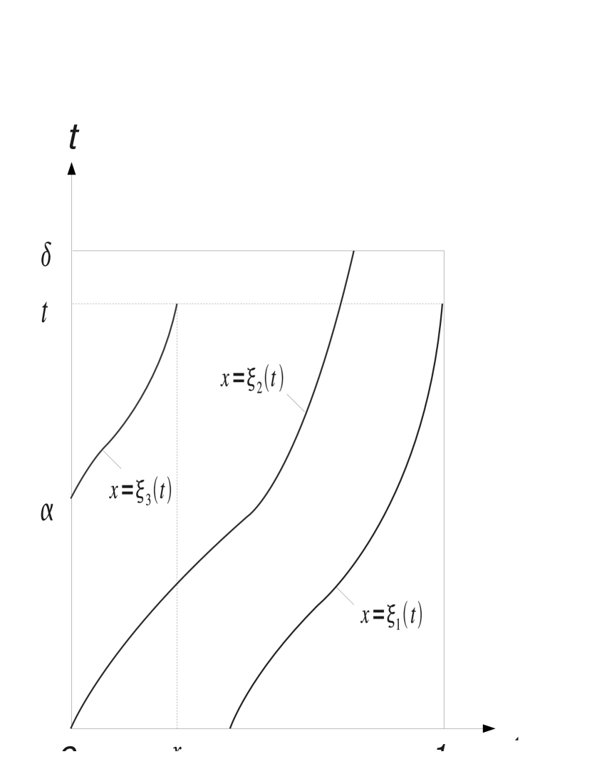
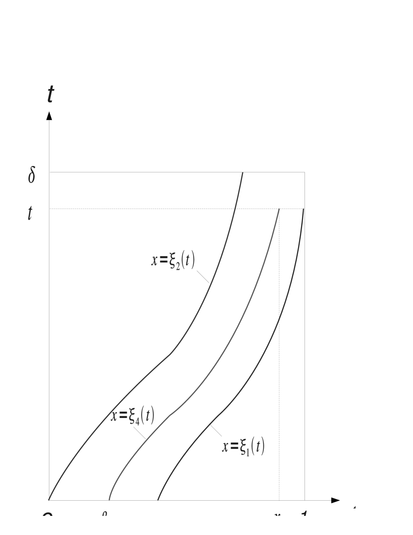
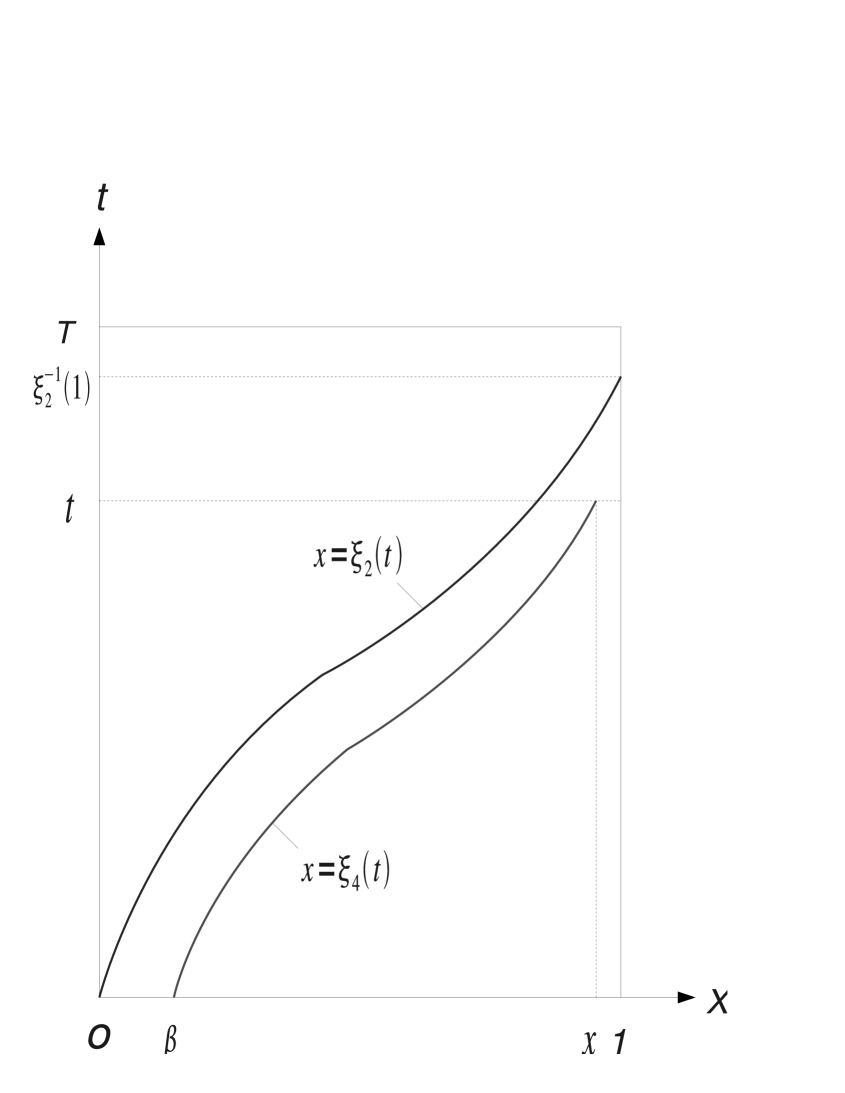
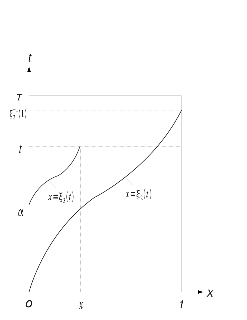
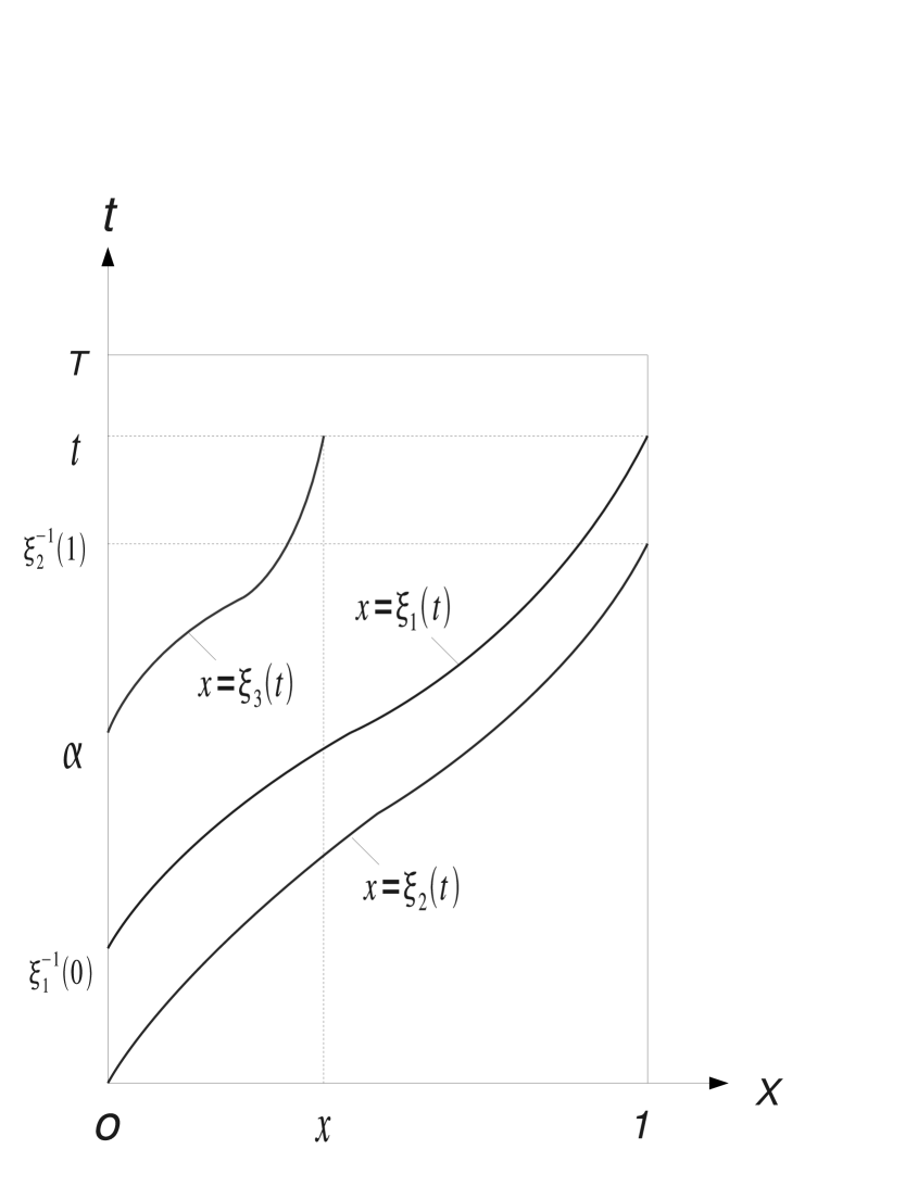
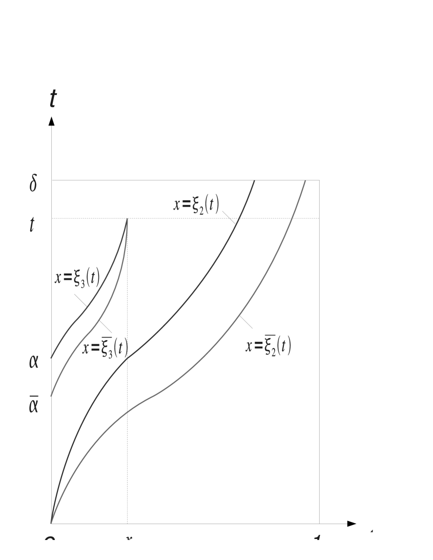
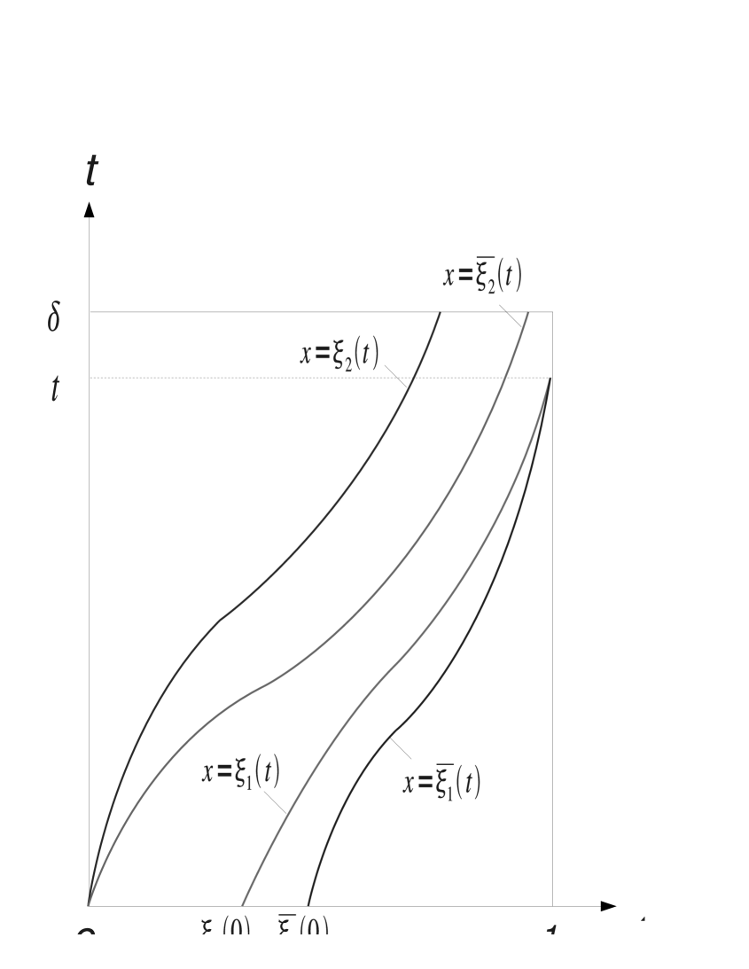
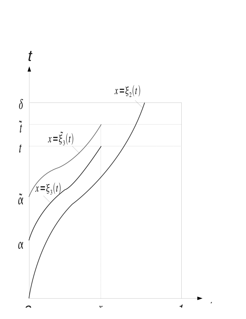
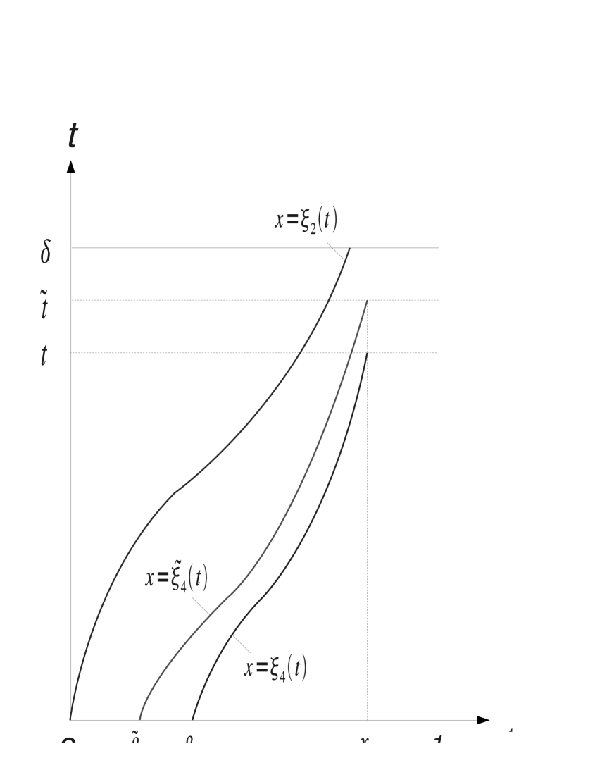
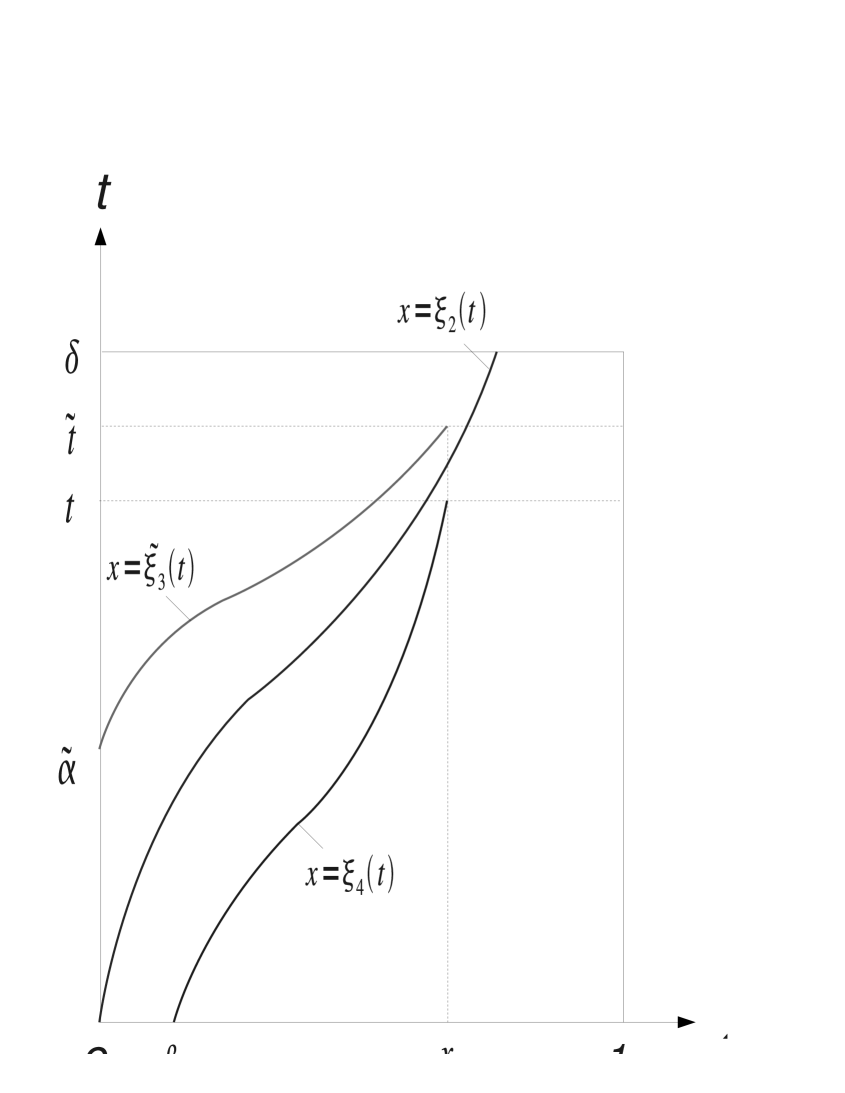
where $\xi_{1}$ (see Fig 2 or Fig 2) represents the characteristic curve passing through $(t,1)$ which is defined by

$$\frac{d\xi_{1}}{ds}=\lambda(\xi_{1}(s),W(s)),\quad\xi_{1}(t)=1.$$ (3.3)

Here we remark that the formulation of $F(W)$ is induced by solving the corresponding linear Cauchy problem (1.1), (1.2) and (1.3) in which $W(\cdot)\in\Omega_{\delta,M}$ is known. It is obvious that $F$ maps into $\Omega_{\delta,M}$ itself if

$$0<\delta\leq\min\Big{\{}\frac{1}{\|\lambda\|_{C^{0}}},T\Big{\}}.$$

Now we prove that, if $\delta$ is small enough, $F$ is a contraction mapping on $\Omega_{\delta,M}$ with respect to the $C^{0}$ norm. Let $W,\overline{W}\in\Omega_{\delta,M}$ and for any fixed $t\in[0,T]$, we define $\overline{\xi}_{1}$ by

$$\frac{d\overline{\xi}_{1}}{ds}=\lambda(\overline{\xi}_{1}(s),\overline{W}(s)),\quad\overline{\xi}_{1}(t)=1.$$

Then, we have for every $t\in[0,\delta]$ that

$$\quad|F(\overline{W})(t)-F(W)(t)|=\Big{|}\int_{1-\int_{0}^{t}\lambda(\xi_{1}(\theta),W(\theta))d\theta}^{1-\int_{0}^{t}\lambda(\overline{\xi}_{1}(\theta),\overline{W}(\theta))d\theta}\rho_{0}(\beta)d\beta\Big{|}$$

$$\leq\|\rho_{0}\|_{L^{\infty}}\cdot\Big{|}\int_{0}^{t}(\lambda(\overline{\xi}_{1}(\theta),\overline{W}(\theta))-\lambda(\xi_{1}(\theta),W(\theta)))d\theta\Big{|}$$

$$\leq t\|\rho_{0}\|_{L^{\infty}}\cdot\Big{(}\|\lambda_{x}\|_{C^{0}}\|\overline{\xi}_{1}-\xi_{1}\|_{C^{0}([0,t])}+\|\lambda_{W}\|_{C^{0}}\|\overline{W}-W\|_{C^{0}([0,\delta])}\Big{)}.$$

By the definitions of $\xi_{1}$ and $\overline{\xi}_{1}$, we obtain

$$\quad\|\overline{\xi}_{1}-\xi_{1}\|_{C^{0}([0,t])}=\sup_{0\leq\theta\leq t}|\overline{\xi}_{1}(\theta)-\xi_{1}(\theta)|$$

$$=\sup_{0\leq\theta\leq t}\Big{|}\int_{\theta}^{t}(\lambda(\overline{\xi}_{1}(\sigma),\overline{W}(\sigma))-\lambda(\xi_{1}(\sigma),W(\sigma)))d\sigma\Big{|}$$

$$\leq t\|\lambda_{x}\|_{C^{0}}\|\overline{\xi}_{1}-\xi_{1}\|_{C^{0}([0,t])}+t\|\lambda_{W}\|_{C^{0}}\|\overline{W}-W\|_{C^{0}([0,\delta])},$$

thus

$$\|\overline{\xi}_{1}-\xi_{1}\|_{C^{0}([0,t])}\leq\frac{t\|\lambda_{W}\|_{C^{0}}}{1-t\|\lambda_{x}\|_{C^{0}}}\cdot\|\overline{W}-W\|_{C^{0}([0,\delta])}.$$ (3.4)

Therefore,

$$|F(\overline{W})(t)-F(W)(t)|\leq\frac{t\|\rho_{0}\|_{L^{\infty}}\|\lambda_{W}\|_{C^{0}}}{1-t\|\lambda_{x}\|_{C^{0}}}\cdot\|\overline{W}-W\|_{C^{0}([0,\delta])},\quad\forall t\in[0,\delta].$$

Let $\delta$ be such that

$$0<\delta\leq\min\Big{\{}\frac{1}{2\|\lambda_{x}\|_{C^{0}}},\frac{1}{4\|\rho_{0}\|_{L^{\infty}}\|\lambda_{W}\|_{C^{0}}},\frac{1}{\|\lambda\|_{C^{0}}},T\Big{\}},$$ (3.5)

then

$$\|F(\overline{W})-F(W)\|_{C^{0}([0,\delta])}\leq\frac{1}{2}\|\overline{W}-W\|_{C^{0}([0,\delta])}.$$

By means of the contraction mapping principle, there exists a unique fixed point $W=F(W)$ in $\Omega_{\delta,M}$:

$$W(t)=F(W)(t)=\int_{0}^{t}u(\alpha)d\alpha+\int_{0}^{1-\int_{0}^{t}\lambda(\xi_{1}(\theta),W(\theta))d\theta}\rho_{0}(\beta)d\beta,\quad\forall t\in[0,\delta].$$

Moreover, $W$ is Lipschitz continuous:

$$W(t)=W(0)+\int_{0}^{t}W^{\prime}(s)ds,$$

with

$$W^{\prime}(t)=u(t)-\lambda(\xi_{1}(t),W(t))\rho_{0}(1-\int_{0}^{t}\lambda(\xi_{1}(\theta),W(\theta))d\theta),\quad t\in[0,\delta],$$

and thus

$$\|W^{\prime}\|_{L^{\infty}(0,\delta)}\leq\|u\|_{L^{\infty}}+\|\lambda\|_{C^{0}}\|\rho_{0}\|_{L^{\infty}}.$$ (3.6)

Now we define the characteristic curve $\xi_{2}$ which passes through the origin (see Fig 2 and Fig 2) by

$$\frac{d\xi_{2}}{ds}=\lambda(\xi_{2}(s),W(s)),\quad\xi_{2}(0)=0.$$ (3.7)

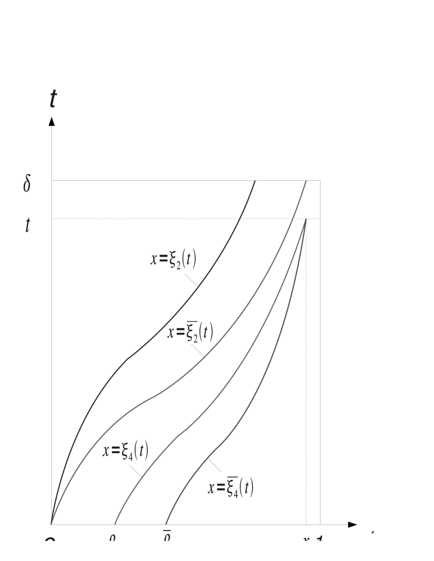
And then for any fixed $t\in[0,\delta]$, we define the characteristic curves $\xi_{3},\xi_{4}$ (see Fig 2 and Fig 2) which pass through $(t,x)$ by

$$\frac{d\xi_{3}}{ds}=\lambda(\xi_{3}(s),W(s)),\quad\xi_{3}(t)=x,\quad\text{for}\ x\in[0,\xi_{2}(t)].$$ (3.8)

$$\frac{d\xi_{4}}{ds}=\lambda(\xi_{4}(s),W(s)),\quad\xi_{4}(t)=x,\quad\text{for}\ x\in[\xi_{2}(t),1].$$ (3.9)

From the uniqueness of the solution to the ordinary differential equation, we know that there exist $\alpha\in[0,\delta]$ and $\beta\in[0,1]$ such that

$$\xi_{3}(\alpha)=0\quad\text{and }\quad\xi_{4}(0)=\beta.$$ (3.10)

Now we define a function $\rho$ by

$$\rho(t,x):=\begin{cases}\displaystyle\frac{u(\alpha)}{\lambda(0,W(\alpha))}\,e^{-\int_{\alpha}^{t}\lambda_{x}(\xi_{3}(\theta),W(\theta))d\theta},\quad&0\leq x\leq\xi_{2}(t),0\leq t\leq\delta,\\ \rho_{0}(\beta)\,e^{-\int_{0}^{t}\lambda_{x}(\xi_{4}(\theta),W(\theta))d\theta},\quad&0\leq\xi_{2}(t)\leq x,0\leq t\leq\delta,\end{cases}$$ (3.11)

which is obviously nonnegative almost everywhere in $(0,\delta)\times(0,1)$. Using the following two lemmas, we can prove that $\rho$ defined by (3.11) is the unique weak solution to the Cauchy problem (1.1), (1.2) and (1.3).

Lemma 3.1.

The function $\rho$ defined by (3.11) is a weak solution to Cauchy problem (1.1), (1.2) and (1.3). Moreover, the weak solution $\rho$ even belongs to $C^{0}([0,\delta];L^{p}(0,1))$ for all $p\in[1,\infty)$ and the following two estimates hold for all $t\in[0,\delta]$:

$$0\leq W(t)=\|\rho(t,\cdot)\|_{L^{1}(0,1)}\leq M,$$ (3.12)

$$\|\rho(t,\cdot)\|_{L^{\infty}(0,1)}\leq e^{T\|\lambda_{x}\|_{C^{0}}}\cdot\max\Big{\{}\|\rho_{0}\|_{L^{\infty}},\frac{\|u\|_{L^{\infty}}}{\overline{\lambda}(M)}\Big{\}}.$$ (3.13)

Lemma 3.2.

The weak solution to Cauchy problem (1.1), (1.2) and (1.3) is unique.

We leave the proofs of Lemma 3.1 and Lemma 3.2 in Appendix.

Now we suppose that we have solved Cauchy problem (1.1), (1.2) and (1.3) to the moment $\tau\in(0,T)$ with the weak solution $\rho\in C^{0}([0,\tau];L^{p}(0,1))\cap L^{\infty}((0,\tau)\times(0,1))$. Similar to Lemma 3.1 and Lemma 3.2, we know that this weak solution is given by

$$\rho(t,x)=\begin{cases}\rho_{0}(\beta)\,e^{-\int_{0}^{t}\lambda_{x}(\xi_{4}(\theta),W(\theta))d\theta},\quad&\text{if}\ 0\leq\xi_{2}(t)\leq x\leq 1,0\leq t\leq\tau,\\ \displaystyle\frac{u(\alpha)}{\lambda(0,W(\alpha))}\,e^{-\int_{\alpha}^{t}\lambda_{x}(\xi_{3}(\theta),W(\theta))d\theta},\quad&\text{else}.\end{cases}$$

Moreover, the two uniform a priori estimates (3.12) and (3.13) hold for all $t\in[0,\tau]$. Hence we can choose $\delta\in(0,T)$ independent of $\tau$ such that (3.5) holds. Applying Lemma 3.1 and Lemma 3.2 again, the weak solution $\rho\in C^{0}([0,\tau];L^{p}(0,1))$, as well as estimates (3.12) and (3.13), is extended to the time interval $[\tau,\tau+\delta]\cap[\tau,T]$. Step by step, we finally have a unique global weak solution $\rho\in C^{0}([0,T];L^{p}(0,1))\cap L^{\infty}((0,T)\times(0,1))$. This finishes the proof of Theorem 3.1. ∎

Remark 3.1.

Let $\rho$ be the weak solution in Theorem 3.1 and $W\in C^{0}([0,T])$ be the total mass function: $W(t)=\int_{0}^{1}\rho(t,x)dx$. Let $\xi_{1},\xi_{2},\xi_{3},\xi_{4}$ and $\alpha,\beta$ be defined by (3.3), (3.7), (3.8), (3.9) and (3.10), respectively. It follows from our proof of Theorem 3.1 that (see Fig 4, Fig 4 and Fig 6)

$$\rho(t,x)=\begin{cases}\rho_{0}(\beta)\,e^{-\int_{0}^{t}\lambda_{x}(\xi_{4}(\theta),W(\theta))d\theta},\quad&\text{if}\ 0\leq\xi_{2}(t)\leq x\leq 1,0\leq t\leq T,\\ \displaystyle\frac{u(\alpha)}{\lambda(0,W(\alpha))}\,e^{-\int_{\alpha}^{t}\lambda_{x}(\xi_{3}(\theta),W(\theta))d\theta},\quad&\text{else}.\end{cases}$$ (3.14)

and the following estimate holds:

$$\|\rho(t,\cdot)\|_{L^{\infty}(0,1)}\leq e^{T\|\lambda_{x}\|_{C^{0}}}\cdot\max\Big{\{}\|\rho_{0}\|_{L^{\infty}},\frac{\|u\|_{L^{\infty}}}{\overline{\lambda}(M)}\Big{\}},\quad\forall t\in[0,T].$$ (3.15)

Moreover, $W(t)$ can be expressed as (see Fig 6)

$$W(t)=\begin{cases}\displaystyle\int_{0}^{t}u(\alpha)d\alpha+\int_{0}^{1-\int_{0}^{t}\lambda(\xi_{1}(\theta),W(\theta))d\theta}\rho_{0}(\beta)d\beta,\quad&0\leq t\leq\xi_{2}^{-1}(1),\\ \displaystyle\int_{\xi_{1}^{-1}(0)}^{t}u(\alpha)d\alpha,&\xi_{2}^{-1}(1)\leq t\leq T,\end{cases}$$ (3.16)

which implies again that

$$0\leq W(t)=\|\rho(t,\cdot)\|_{L^{1}(0,1)}\leq M,\quad\forall t\in[0,T].$$ (3.17)

Finally, $W$ is Lipschitz continuous:

$$W(t)=W(0)+\int_{0}^{t}W^{\prime}(s)ds,$$

where (see Fig 6)

$$W^{\prime}(t)=\begin{cases}\displaystyle u(t)-\lambda(\xi_{1}(t),W(t))\rho_{0}(1-\int_{0}^{t}\lambda(\xi_{1}(\theta),W(\theta))d\theta),\quad&0\leq t\leq\xi_{2}^{-1}(1),\\ \displaystyle u(t)-u(\xi_{1}^{-1}(0))\frac{\lambda(1,W(t))}{\lambda(0,W(\xi_{1}^{-1}(0)))}\,e^{-\int_{\xi_{1}^{-1}(0)}^{t}\lambda_{x}(\xi_{1}(\theta),W(\theta))\,d\theta},&\xi_{2}^{-1}(1)\leq t\leq T\end{cases}$$

and

$$\|W^{\prime}\|_{L^{\infty}(0,T)}\leq\|u\|_{L^{\infty}}+\|\lambda\|_{C^{0}}\cdot\max\Big{\{}\|\rho_{0}\|_{L^{\infty}},\frac{\|u\|_{L^{\infty}}}{\overline{\lambda}(M)}\,e^{T\|\lambda_{x}\|_{C^{0}}}\Big{\}}<\infty.$$ (3.18)

Remark 3.2.

(Hidden regularity.) From the definition of the weak solution, we can expect $\rho\in L^{\infty}((0,T)\times(0,1))=L^{\infty}(0,1;L^{\infty}(0,T))$. In fact, under the assumptions of Theorem 3.1, we have the hidden regularity that $\rho\in C^{0}([0,1];L^{p}(0,T))$ for all $p\in[1,\infty)$ so that the function $t\mapsto\rho(t,x)\in L^{p}(0,T)$ is well defined for every fixed $x\in[0,1]$. The proof of the hidden regularity is quite similar to our proof of $\rho\in C^{0}([0,T];L^{p}(0,1))$ by means of the implicit expressions (3.14) for $\rho$ and (3.16) for $W(t)$ (see also (3.18) when $T$ is large).

Remark 3.3.

If $\rho_{0}\in C^{0}([0,1])$ and $u\in C^{0}([0,T])$ are nonnegative and the $C^{0}$ compatibility condition is satisfied at the origin:

$$\frac{u(0)}{\lambda(0,W(0))}-\rho_{0}(0)=0,$$

where $W(0)=\int_{0}^{1}\rho_{0}(x)dx,$ then Cauchy problem (1.1), (1.2) and (1.3) admits a unique nonnegative solution $\rho\in C^{0}([0,T]\times[0,1])$. If, furthermore, $\rho_{0}\in C^{1}([0,1])$ and $u\in C^{1}([0,T])$ are nonnegative and the $C^{1}$ compatibility conditions are satisfied at the origin:

$$\begin{cases}\displaystyle\frac{u(0)}{\lambda(0,W(0))}-\rho_{0}(0)=0,\\ \displaystyle\frac{u^{\prime}(0)\lambda(0,W(0))-u(0)\lambda_{W}(0,W(0))W^{\prime}(0)}{|\lambda(0,W(0))|^{2}}+\lambda(0,W(0))\rho_{0}^{\prime}(0)+\lambda_{x}(0,W(0))\rho_{0}(0)=0,\end{cases}$$

where $W(0)=\int_{0}^{1}\rho_{0}(x)dx$ and $W^{\prime}(0)=u(0)-\rho_{0}(1)\lambda(1,W(0))$, then Cauchy problem (1.1), (1.2) and (1.3) admits a unique nonnegative classical solution $\rho\in C^{1}([0,T]\times[0,1])$.

4 Stability with respect to the initial and boundary data

In this section, we study the stability (or continuous dependence) of both the solution $\rho$ itself and the out-flux $y$ with respect to $\rho_{0}$ and $u$. That is to say: if the initial and boundary data are slightly perturbed, are the solution $\rho$ and the out-flux $y$ also slightly perturbed?

Let $\overline{\rho}$ be the weak solution to the Cauchy problem with the perturbed initial and boundary conditions

$$\begin{cases}\overline{\rho}_{t}(t,x)+(\overline{\rho}(t,x)\lambda(x,\overline{W}(t)))_{x}=0,\quad&t\geq 0,0\leq x\leq 1,\\ \overline{\rho}(0,x)=\overline{\rho}_{0}(x),\quad&0\leq x\leq 1,\\ \overline{\rho}(t,0)\lambda(0,\overline{W}(t))=\overline{u}(t),\quad&0\leq t\leq T,\end{cases}$$ (4.1)

where $\overline{W}(t):=\int_{0}^{1}\overline{\rho}(t,x)dx$. We denote that $\overline{y}(t):=\overline{\rho}(1,t)\lambda(1,\overline{W}(t))$. We also define the corresponding characteristics with respect to the perturbed solution $\overline{\rho}$ : $\overline{\xi}_{1}$ (as (3.3)), $\overline{\xi}_{2}$ (as (3.7)), $(\overline{\xi}_{3},\overline{\alpha})$ (as (3.8) and (3.10)) and $(\overline{\xi}_{4},\overline{\beta})$ (as (3.9) and (3.10)), respectively.

First we have the following theorem on the stability of the weak solution $\rho$.

Theorem 4.1.

For any $\varepsilon>0$, $p\in[1,\infty)$ and any $K>0$ such that

$$\|\rho_{0}\|_{L^{\infty}(0,1)}+\|u\|_{L^{\infty}(0,T)}\leq K,\quad\|\overline{\rho}_{0}\|_{L^{\infty}(0,1)}+\|\overline{u}\|_{L^{\infty}(0,T)}\leq K,$$ (4.2)

there exists $\eta=\eta(\varepsilon,p,K)>0$ small enough such that, if

$$\|\overline{\rho}_{0}-\rho_{0}\|_{L^{p}(0,1)}+\|\overline{u}-u\|_{L^{p}(0,T)}<\eta,$$ (4.3)

then

$$\|\overline{\rho}(t,\cdot)-\rho(t,\cdot)\|_{L^{p}(0,1)}<\varepsilon,\quad\forall t\in[0,T].$$ (4.4)

Proof:.

Solving Cauchy problem (4.1), we know from (3.17) and (4.2) that

$$0\leq\overline{W}(t)\leq\|\overline{\rho}_{0}\|_{L^{1}(0,1)}+\|\overline{u}\|_{L^{1}(0,T)}\leq K,\quad\forall t\in[0,T].$$ (4.5)

Replacing $M$ by $K$ in the definitions of $\overline{\lambda}(M)$ and $\|\lambda\|_{C^{0}},\|\lambda_{x}\|_{C^{0}},\|\lambda_{W}\|_{C^{0}}$ (see Section 2), we introduce some new notations as $\overline{\lambda}(K)$ and (still) $\|\lambda\|_{C^{0}},\|\lambda_{x}\|_{C^{0}},\|\lambda_{W}\|_{C^{0}}$ in this section.

We first prove the stability of the weak solution for small time. Let $\delta$ be chosen by (3.5). For any fixed $t\in[0,\delta]$, we suppose that $\xi_{2}(t)<\overline{\xi}_{2}(t)$ (the case that $\xi_{2}(t)\geq\overline{\xi}_{2}(t)$ can be treated similarly). In order to estimate $\|\overline{\rho}(t,\cdot)-\rho(t,\cdot)\|_{L^{p}(0,1)}$ for $p\in[1,\infty)$, we need to estimate $\int_{0}^{\xi_{2}(t)}|\overline{\rho}(t,x)-\rho(t,x)|^{p}dx$, $\int_{\xi_{2}(t)}^{\overline{\xi}_{2}(t)}|\overline{\rho}(t,x)-\rho(t,x)|^{p}dx$ and $\int_{\overline{\xi}_{2}(t)}^{1}|\overline{\rho}(t,x)-\rho(t,x)|^{p}dx$, successively.

For almost every $x\in[0,\xi_{2}(t)]$, we know from Remark 3.1 that (see Fig 6)

$$\quad|\overline{\rho}(t,x)-\rho(t,x)|$$

$$=\Big{|}\frac{\overline{u}(\overline{\alpha})}{\lambda(0,\overline{W}(\overline{\alpha}))}\,e^{-\int_{\overline{\alpha}}^{t}\lambda_{x}(\overline{\xi}_{3}(\theta),\overline{W}(\theta))\,d\theta}-\frac{u(\alpha)}{\lambda(0,W(\alpha))}\,e^{-\int_{\alpha}^{t}\lambda_{x}(\xi_{3}(\theta),W(\theta))\,d\theta}\Big{|}$$

$$\leq\frac{|\overline{u}(\overline{\alpha})-u(\alpha)|}{\lambda(0,\overline{W}(\overline{\alpha}))}\,e^{-\int_{\overline{\alpha}}^{t}\lambda_{x}(\overline{\xi}_{3}(\theta),\overline{W}(\theta))\,d\theta}+\Big{|}\frac{u(\alpha)}{\lambda(0,\overline{W}(\overline{\alpha}))}-\frac{u(\alpha)}{\lambda(0,W(\alpha))}\Big{|}\,e^{-\int_{\overline{\alpha}}^{t}\lambda_{x}(\overline{\xi}_{3}(\theta),\overline{W}(\theta))\,d\theta}$$

$$\quad+\frac{|u(\alpha)|}{\lambda(0,W(\alpha))}\Big{|}e^{-\int_{\overline{\alpha}}^{t}\lambda_{x}(\overline{\xi}_{3}(\theta),\overline{W}(\theta))\,d\theta}-e^{-\int_{\alpha}^{t}\lambda_{x}(\xi_{3}(\theta),W(\theta))\,d\theta}\Big{|}$$

$$\leq C|\overline{u}(\overline{\alpha})-u(\alpha)|+C|u(\alpha)||\overline{W}(\overline{\alpha})-W(\alpha)|$$

$$\quad+C|u(\alpha)|\Big{|}\int_{\overline{\alpha}}^{t}\lambda_{x}(\overline{\xi}_{3}(\theta),\overline{W}(\theta))\,d\theta-\int_{\alpha}^{t}\lambda_{x}(\xi_{3}(\theta),W(\theta))\,d\theta\Big{|}.$$

Here and hereafter in this section, we denote by $C$ various constants which do not depend on $t,x,\rho,\overline{\rho}$ but may depend on $p$ and $K$.

For the given $u\in L^{\infty}(0,T)$, let $\{u_{n}\}_{n=1}^{\infty}\subset C^{1}([0,T])$ be such that $u_{n}\rightarrow u$ in $L^{p}(0,T)$. And for the given $\lambda\in C^{1}([0,1]\times[0,\infty))$, let $\{v_{n}\}_{n=1}^{\infty}\subset C^{1}([0,1]\times[0,K])$ be such that $v_{n}\rightarrow\lambda_{x}$ in $C^{0}([0,1]\times[0,K])$. Using sequences $\{u_{n}\}_{n=1}^{\infty}$, $\{v_{n}\}_{n=1}^{\infty}$ and (3.6), we obtain for almost every $x\in[0,\xi_{2}(t)]$ that

$$\quad|\overline{\rho}(t,x)-\rho(t,x)|$$

$$\leq C|\overline{u}(\overline{\alpha})-u(\overline{\alpha})|+C|u_{n}(\overline{\alpha})-u(\overline{\alpha})|+C|u_{n}(\alpha)-u(\alpha)|$$

$$\quad+C|u_{n}(\overline{\alpha})-u_{n}(\alpha)|+C|\overline{W}(\overline{\alpha})-W(\overline{\alpha})|+C|W(\overline{\alpha})-W(\alpha)|$$

$$\quad+C|u(\alpha)|\int_{\overline{\alpha}}^{t}|v_{n}(\overline{\xi}_{3}(\theta),\overline{W}(\theta))-\lambda_{x}(\overline{\xi}_{3}(\theta),\overline{W}(\theta))|\,d\theta$$

$$\quad+C|u(\alpha)|\int_{\alpha}^{t}|v_{n}(\xi_{3}(\theta),W(\theta))-\lambda_{x}(\xi_{3}(\theta),W(\theta))|\,d\theta$$

$$\quad+C|u(\alpha)|\Big{|}\int_{\overline{\alpha}}^{t}v_{n}(\overline{\xi}_{3}(\theta),\overline{W}(\theta))\,d\theta-\int_{\alpha}^{t}v_{n}(\xi_{3}(\theta),W(\theta))\,d\theta\Big{|}$$

$$\leq C|\overline{u}(\overline{\alpha})-u(\overline{\alpha})|+C|u_{n}(\overline{\alpha})-u(\overline{\alpha})|+C|u_{n}(\alpha)-u(\alpha)|$$

$$\quad+C|u(\alpha)|\|v_{n}-\lambda_{x}\|_{C^{0}([0,1]\times[0,K])}+C_{n}|\overline{\alpha}-\alpha|+C_{n}|u(\alpha)||\overline{\alpha}-\alpha|$$

$$\quad+C_{n}|u(\alpha)|\|\overline{\xi}_{3}-\xi_{3}\|_{C^{0}([\overline{\alpha},t])}+C_{n}|u(\alpha)|\|\overline{W}-W\|_{C^{0}([0,\delta])}.$$ (4.6)

Here and hereafter in this section, we denote by $C_{n}$ various constants which do not depend on $t,x,\rho,\overline{\rho}$ but may depend on $p,K$ and $n$ (the index of the corresponding sequences, e.g. $\{u_{n}\}_{n=1}^{\infty}$, $\{v_{n}\}_{n=1}^{\infty}$ and so on).

A similar estimate as (3.4) gives us

$$\|\overline{\xi}_{3}-\xi_{3}\|_{C^{0}([\overline{\alpha},t])}\leq\frac{t\|\lambda_{W}\|_{C^{0}}}{1-t\|\lambda_{x}\|_{C^{0}}}\cdot\|\overline{W}-W\|_{C^{0}([0,\delta])}.$$ (4.7)

From the fact that

$$\overline{\xi}_{3}(t)=\int_{\overline{\alpha}}^{t}\lambda(\overline{\xi}_{3}(\theta),\overline{W}(\theta))\,d\theta=x=\xi_{3}(t)=\int_{\alpha}^{t}\lambda(\xi_{3}(\theta),W(\theta))\,d\theta$$

and the definition of $\overline{\lambda}(K)$, we get also that

$$|\overline{\alpha}-\alpha| \leq\frac{1}{\overline{\lambda}(K)}\int_{\alpha}^{\overline{\alpha}}\lambda(\xi_{3}(\theta),W(\theta))\,d\theta$$

$$=\frac{1}{\overline{\lambda}(K)}\int_{\overline{\alpha}}^{t}(\lambda(\overline{\xi}_{3}(\theta),\overline{W}(\theta))-\lambda(\xi_{3}(\theta),W(\theta)))\,d\theta$$

$$\leq\frac{1}{\overline{\lambda}(K)}\Big{(}t\|\lambda_{x}\|_{C^{0}}\|\overline{\xi}_{3}-\xi_{3}\|_{C^{0}([\overline{\alpha},t])}+t\|\lambda_{W}\|_{C^{0}}\|\overline{W}-W\|_{C^{0}([0,\delta])}\Big{)}$$

$$\leq\frac{t\|\lambda_{W}\|_{C^{0}}}{\overline{\lambda}(K)(1-t\|\lambda_{x}\|_{C^{0}})}\cdot\|\overline{W}-W\|_{C^{0}([0,\delta])}.$$ (4.8)

On the other hand, by (3.16) and Hölder inequality, we have for every $t\in[0,\delta]$ that

$$\quad|\overline{W}(t)-W(t)|$$

$$=\Big{|}\int_{0}^{t}(\overline{u}(\sigma)-u(\sigma))d\sigma+\int_{0}^{1-\int_{0}^{t}\lambda(\overline{\xi}_{1}(\theta),\overline{W}(\theta))\,d\theta}\overline{\rho}_{0}(\sigma)\,d\sigma-\int_{0}^{1-\int_{0}^{t}\lambda(\xi_{1}(\theta),W(\theta))\,d\theta}\rho_{0}(\sigma)\,d\sigma\Big{|}$$

$$\leq\delta^{\frac{1}{q}}\|\overline{u}-u\|_{L^{p}(0,T)}+\|\overline{\rho}_{0}-\rho_{0}\|_{L^{p}(0,1)}+\|\rho_{0}\|_{L^{\infty}}\int_{0}^{t}|\lambda(\overline{\xi}_{1}(\theta),\overline{W}(\theta))-\lambda(\xi_{1}(\theta),W(\theta))|\,d\theta$$

$$\leq\delta^{\frac{1}{q}}\|\overline{u}-u\|_{L^{p}(0,T)}+\|\overline{\rho}_{0}-\rho_{0}\|_{L^{p}(0,1)}$$

$$\quad+\delta\|\rho_{0}\|_{L^{\infty}}(\|\lambda_{x}\|_{C^{0}}\|\overline{\xi}_{1}-\xi_{1}\|_{C^{0}([0,t])}+\|\lambda_{W}\|_{C^{0}}\|\overline{W}-W\|_{C^{0}([0,\delta])}),$$

where $q$ satisfies $\frac{1}{p}+\frac{1}{q}=1$. By the definitions of $\xi_{1}$ and $\overline{\xi}_{1}$, we still have (3.4), thus

$$\quad\|\overline{W}-W\|_{C^{0}([0,\delta])}=\sup_{t\in[0,\delta]}|\overline{W}(t)-W(t)|$$

$$\leq\frac{1-\delta\|\lambda_{x}\|_{C^{0}}}{1-\delta(\|\lambda_{x}\|_{C^{0}}+\|\rho_{0}\|_{L^{\infty}}\|\lambda_{W}\|_{C^{0}})}\cdot(\delta^{\frac{1}{q}}\|\overline{u}-u\|_{L^{p}(0,T)}+\|\overline{\rho}_{0}-\rho_{0}\|_{L^{p}(0,1)}).$$

and furthermore, from the choice (3.5) of $\delta$,

$$\|\overline{W}-W\|_{C^{0}([0,\delta])}\leq C\|\overline{u}-u\|_{L^{p}(0,T)}+C\|\overline{\rho}_{0}-\rho_{0}\|_{L^{p}(0,1)}.$$ (4.9)

Therefore, combining (4), (4.7), (4) and (4.9) all together and using Lemma A.1, we obtain easily that

$$\quad\int_{0}^{\xi_{2}(t)}|\overline{\rho}(t,x)-\rho(t,x)|^{p}dx$$

$$\leq C\|u_{n}-u\|^{p}_{L^{p}(0,T)}+C\|v_{n}-\lambda_{x}\|^{p}_{C^{0}([0,1]\times[0,K])}$$

$$\quad+C_{n}\|\overline{u}-u\|^{p}_{L^{p}(0,T)}+C_{n}\|\overline{\rho}_{0}-\rho_{0}\|^{p}_{L^{p}(0,1)}.$$ (4.10)

For almost every $x\in[\overline{\xi}_{2}(t),1]$, we know from Remark 3.1 that (see Fig 8)

$$\quad|\overline{\rho}(t,x)-\rho(t,x)|=\Big{|}\overline{\rho}_{0}(\overline{\beta})e^{-\int_{0}^{t}\lambda_{x}(\overline{\xi}_{4}(\theta),\overline{W}(\theta))\,d\theta}-\rho_{0}(\beta)e^{-\int_{0}^{t}\lambda_{x}(\xi_{4}(\theta),W(\theta))\,d\theta}\Big{|}$$

$$\leq|\overline{\rho}_{0}(\overline{\beta})-\rho_{0}(\beta)|e^{-\int_{0}^{t}\lambda_{x}(\overline{\xi}_{4}(\theta),\overline{W}(\theta))\,d\theta}+|\rho_{0}(\beta)|\Big{|}e^{-\int_{0}^{t}\lambda_{x}(\overline{\xi}_{4}(\theta),\overline{W}(\theta))\,d\theta}-e^{-\int_{0}^{t}\lambda_{x}(\xi_{4}(\theta),W(\theta))\,d\theta}\Big{|}$$

$$\leq C|\overline{\rho}_{0}(\overline{\beta})-\rho_{0}(\overline{\beta})|+C|\rho_{0}(\overline{\beta})-\rho_{0}(\beta)|$$

$$\quad+C|\rho_{0}(\beta)|\Big{|}\int_{0}^{t}(\lambda_{x}(\overline{\xi}_{4}(\theta),\overline{W}(\theta))-\lambda_{x}(\xi_{4}(\theta),W(\theta)))\,d\theta\Big{|}.$$

For the given $\rho_{0}\in L^{\infty}(0,1)$, we let $\{\rho_{0}^{n}\}_{n=1}^{\infty}\subset C^{1}([0,1])$ be such that $\rho_{0}^{n}\rightarrow\rho_{0}$ in $L^{p}(0,1)$. With the help of sequences $\{\rho^{n}_{0}\}_{n=1}^{\infty}$, $\{v_{n}\}_{n=1}^{\infty}$, we obtain for almost every $x\in[\overline{\xi}_{2}(t),1]$ that

$$\quad|\overline{\rho}(t,x)-\rho(t,x)|$$

$$\leq C|\overline{\rho}_{0}(\overline{\beta})-\rho_{0}(\overline{\beta})|+C|\rho_{0}^{n}(\overline{\beta})-\rho_{0}(\overline{\beta})|+C|\rho_{0}^{n}(\beta)-\rho_{0}(\beta)|+C|\rho_{0}^{n}(\overline{\beta})-\rho_{0}^{n}(\beta)|$$

$$\quad+C|\rho_{0}(\beta)|\int_{0}^{t}|v_{n}(\overline{\xi}_{4}(\theta),\overline{W}(\theta))-\lambda_{x}(\overline{\xi}_{4}(\theta),\overline{W}(\theta))|\,d\theta$$

$$\quad+C|\rho_{0}(\beta)|\int_{0}^{t}|v_{n}(\xi_{4}(\theta),W(\theta))-\lambda_{x}(\xi_{4}(\theta),W(\theta))|\,d\theta$$

$$\quad+C|\rho_{0}(\beta)|\int_{0}^{t}|v_{n}(\overline{\xi}_{4}(\theta),\overline{W}(\theta))-v_{n}(\xi_{4}(\theta),W(\theta))|\,d\theta$$

$$\leq C|\overline{\rho}_{0}(\overline{\beta})-\rho_{0}(\overline{\beta})|+C|\rho_{0}^{n}(\overline{\beta})-\rho_{0}(\overline{\beta})|+C|\rho_{0}^{n}(\beta)-\rho_{0}(\beta)|+C|\rho_{0}(\beta)|\|v_{n}-\lambda_{x}\|_{C^{0}([0,1]\times[0,K])}$$

$$\quad+C_{n}|\overline{\beta}-\beta|+C_{n}|\rho_{0}(\beta)|\|\overline{\xi}_{4}-\xi_{4}\|_{C^{0}([0,t])}+C_{n}|\rho_{0}(\beta)|\|\overline{W}-W\|_{C^{0}([0,\delta])}.$$ (4.11)

Similar to (3.4), we have

$$\|\overline{\xi}_{4}-\xi_{4}\|_{C^{0}([0,t])}\leq\frac{t\|\lambda_{W}\|_{C^{0}}}{1-t\|\lambda_{x}\|_{C^{0}}}\cdot\|\overline{W}-W\|_{C^{0}([0,\delta])},$$ (4.12)

and in particular,

$$|\overline{\beta}-\beta|=|\overline{\xi}_{4}(0)-\xi_{4}(0)|\leq\frac{t\|\lambda_{W}\|_{C^{0}}}{1-t\|\lambda_{x}\|_{C^{0}}}\cdot\|\overline{W}-W\|_{C^{0}([0,\delta])}.$$ (4.13)

Therefore, by the choice (3.5) of $\delta$, together with estimates (4.9), (4),(4.12), (4.13) and Lemma A.2, we get immediately that

$$\quad\int_{\overline{\xi}_{2}(t)}^{1}|\overline{\rho}(t,x)-\rho(t,x)|^{p}dx$$

$$\leq C\|\rho_{0}^{n}-\rho_{0}\|^{p}_{L^{p}(0,1)}+C\|v_{n}-\lambda_{x}\|^{p}_{C^{0}([0,1]\times[0,K])}$$

$$\quad+C_{n}\|\overline{u}-u\|^{p}_{L^{p}(0,T)}+C_{n}\|\overline{\rho}_{0}-\rho_{0}\|^{p}_{L^{p}(0,1)}.$$ (4.14)

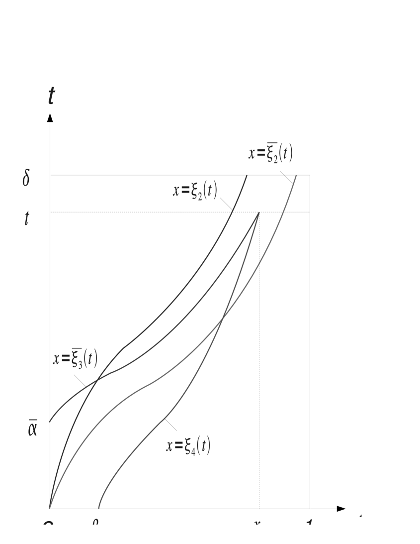
Now it is left to estimate $\int_{\xi_{2}(t)}^{\overline{\xi}_{2}(t)}|\overline{\rho}(t,x)-\rho(t,x)|^{p}dx$ (see Fig 8). Obviously, we have

$$\int_{\xi_{2}(t)}^{\overline{\xi}_{2}(t)}|\overline{\rho}(t,x)-\rho(t,x)|^{p}dx\leq\int_{\xi_{2}(t)}^{x}|\overline{\rho}(t,x)-\rho(t,x)|^{p}dx+\int_{x}^{\overline{\xi}_{2}(t)}|\overline{\rho}(t,x)-\rho(t,x)|^{p}dx.$$ (4.15)

Then similar to estimates (4) and (4), we get easily from (4.15) that

$$\quad\int_{\xi_{2}(t)}^{\overline{\xi}_{2}(t)}|\overline{\rho}(t,x)-\rho(t,x)|^{p}dx$$

$$\leq C\|\rho_{0}^{n}-\rho_{0}\|^{p}_{L^{p}(0,1)}+C\|u_{n}-u\|^{p}_{L^{p}(0,T)}+C\|v_{n}-\lambda_{x}\|^{p}_{C^{0}([0,1]\times[0,K])}$$

$$\quad+C_{n}\|\overline{u}-u\|^{p}_{L^{p}(0,T)}+C_{n}\|\overline{\rho}_{0}-\rho_{0}\|^{p}_{L^{p}(0,1)}.$$ (4.16)

Summarizing estimates (4),(4) and (4), finally we prove for any fixed $t\in[0,\delta]$ with $\delta$ satisfying (3.5) that

$$\quad\|\overline{\rho}(t,\cdot)-\rho(t,\cdot)\|^{p}_{L^{p}(0,1)}$$

$$\leq C\|\rho_{0}^{n}-\rho_{0}\|^{p}_{L^{p}(0,1)}+C\|u_{n}-u\|^{p}_{L^{p}(0,T)}+C\|v_{n}-\lambda_{x}\|^{p}_{C^{0}([0,1]\times[0,K])}$$

$$\quad+C_{n}\|\overline{u}-u\|^{p}_{L^{p}(0,T)}+C_{n}\|\overline{\rho}_{0}-\rho_{0}\|^{p}_{L^{p}(0,1)}.$$ (4.17)

Now if we take $n$ large enough and then $\eta$ in (4.3) small enough, the right-hand side of (4) can be smaller than any given constant $\varepsilon>0$.

In order to obtain the global stability (4.4) from (4), it suffices, according to (3.5), to prove uniform a priori estimates for $\|\rho(t,\cdot)\|_{L^{1}{(0,1)}}$, $\|\rho(t,\cdot)\|_{L^{\infty}(0,1)}$, $\|\overline{\rho}(t,\cdot)\|_{L^{1}{(0,1)}}$, and $\|\overline{\rho}(t,\cdot)\|_{L^{\infty}(0,1)}$. In fact the desired a priori estimates are available by Remark 3.1 (see estimates (3.15) and (3.17)), hence we finally reach (4.4). This finishes the proof of Theorem 4.1.

∎

We also have the stability on the out-flux $y$.

Theorem 4.2.

For any $\varepsilon>0$, $p\in[1,\infty)$ and any $K$ such that (4.2) holds, there exists $\eta=\eta(\varepsilon,p,K))>0$ small enough such that, if (4.3) holds, then

$$\|\overline{y}-y\|_{L^{p}(0,T)}<\varepsilon.$$ (4.18)

Proof:.

First, we prove $\|\overline{y}-y\|_{L^{p}(0,\delta)}<\varepsilon$ for $\delta$ small. Let $\delta$ be such that (3.5) holds. For any fixed $t\in[0,\delta]$, without loss of generality, we suppose that $\xi_{2}(t)<\overline{\xi}_{2}(t)$ (the case that $\xi_{2}(t)\geq\overline{\xi}_{2}(t)$ can be treated similarly). By Remark 3.1, we have for almost every $t\in[0,\delta]$ that (see Fig 10)

$$\quad|\overline{y}(t)-y(t)|$$

$$=|\overline{\rho}(t,1)\lambda(1,\overline{W}(t))-\rho(t,1)\lambda(1,W(t))|$$

$$\leq C|\overline{\rho}(t,1)-\rho(t,1)|+C|\rho(t,1)|\|\overline{W}-W\|_{C^{0}([0,\delta])}$$

$$=C\Big{|}\overline{\rho}_{0}(\overline{\xi}_{1}(0))e^{-\int_{0}^{t}\lambda_{x}(\overline{\xi}_{1}(\theta),\overline{W}(\theta))d\theta}-\rho_{0}(\xi_{1}(0))e^{-\int_{0}^{t}\lambda_{x}(\xi_{1}(\theta),W(\theta))d\theta}\Big{|}$$

$$\quad+C|\rho(t,1)|\|\overline{W}-W\|_{C^{0}([0,\delta])}$$

$$\leq C|\overline{\rho}_{0}(\overline{\xi}_{1}(0))-\rho_{0}(\xi_{1}(0))|+C|\rho(t,1)|\|\overline{W}-W\|_{C^{0}([0,\delta])}$$

$$\quad+C|\rho_{0}(\xi_{1}(0))|\Big{|}\int_{0}^{t}(\lambda_{x}(\overline{\xi}_{1}(\theta),\overline{W}(\theta))-\lambda_{x}(\xi_{1}(\theta),W(\theta)))d\theta\Big{|}.$$

Then using sequences $\{\rho_{0}^{n}\}_{n=1}^{\infty}$, $\{v_{n}\}_{n=1}^{\infty}$, we obtain

$$\quad|\overline{y}(t)-y(t)|$$

$$\leq C|\overline{\rho}_{0}(\overline{\xi}_{1}(0))-\rho_{0}(\overline{\xi}_{1}(0))|+C|\rho_{0}^{n}(\overline{\xi}_{1}(0))-\rho_{0}(\overline{\xi}_{1}(0))|+C|\rho_{0}^{n}(\xi_{1}(0))-\rho_{0}(\xi_{1}(0))|$$

$$\quad+C|\rho_{0}^{n}(\overline{\xi}_{1}(0))-\rho_{0}^{n}(\xi_{1}(0))|+C|\rho(t,1)|\|\overline{W}-W\|_{C^{0}([0,\delta])}$$

$$\quad+C|\rho_{0}(\xi_{1}(0))|\int_{0}^{t}|v_{n}(\overline{\xi}_{1}(\theta),\overline{W}(\theta))-v_{n}(\xi_{1}(\theta),W(\theta))|d\theta$$

$$\quad+C|\rho_{0}(\xi_{1}(0))|\int_{0}^{t}|v_{n}(\overline{\xi}_{1}(\theta),\overline{W}(\theta))-\lambda_{x}(\overline{\xi}_{1}(\theta),\overline{W}(\theta))|d\theta$$

$$\quad+C|\rho_{0}(\xi_{1}(0))|\int_{0}^{t}|v_{n}(\xi_{1}(\theta),W(\theta))-\lambda_{x}(\xi_{1}(\theta),W(\theta))|d\theta,$$

$$\leq C|\overline{\rho}_{0}(\overline{\xi}_{1}(0))-\rho_{0}(\overline{\xi}_{1}(0))|+C|\rho_{0}^{n}(\overline{\xi}_{1}(0))-\rho_{0}(\overline{\xi}_{1}(0))|$$

$$\quad+C|\rho_{0}^{n}(\xi_{1}(0))-\rho_{0}(\xi_{1}(0))|+C|\rho_{0}(\xi_{1}(0))|\|v_{n}-\lambda_{x}\|_{C^{0}([0,1]\times[0,K])}$$

$$\quad+C_{n}|\rho_{0}(\xi_{1}(0))|\|\overline{\xi}_{1}-\xi_{1}\|_{C^{0}([0,t])}+C_{n}|\rho_{0}(\xi_{1}(0))|\|\overline{W}-W\|_{C^{0}([0,\delta])},$$

which results in

$$\quad\int_{0}^{\delta}|\overline{y}(t)-y(t)|^{p}\,dt$$

$$\leq C\|\rho_{0}^{n}-\rho_{0}\|^{p}_{L^{p}(0,1)}+C\|v_{n}-\lambda_{x}\|^{p}_{C^{0}([0,1]\times[0,K])}+C_{n}\|\overline{\rho}_{0}-\rho_{0}\|^{p}_{L^{p}(0,1)}+C_{n}\|\overline{u}-u\|^{p}_{L^{p}(0,T)}$$

with the help of (3.4) and (4.9). Obviously, $\|\overline{y}-y\|_{L^{p}(0,\delta)}<\varepsilon$ holds if we let $n$ large enough and then $\eta>0$ in (4.3) small enough.

In a same way, we can prove for every $\tau\in[0,T-\delta]$ by applying Theorem 4.1 that

$$\|\overline{y}-y\|_{L^{p}(\tau,\tau+\delta)}<\varepsilon$$

if $\delta$ satisfies (3.5) (independent of $\tau$). Step by step, we finally prove (4.18).

∎

5 $L^{p}$-optimal control for demand tracking problem

Let $T>0$ and $\rho_{0}\in L^{\infty}_{+}(0,1)$ be given. According to Theorem 3.1, for every $u\in L^{\infty}_{+}(0,T)$, Cauchy problem (1.1),(1.2) and (1.3) admits a unique weak solution $L^{\infty}((0,T)\times(0,1))\cap\rho\in C^{0}([0,T],L^{p}(0,1))\cap C^{0}([0,1],L^{p}(0,T))$ for all $p\in[1,\infty)$.

For any fixed given demand $y_{d}\in L^{\infty}(0,T)$, initial data $\rho_{0}\in L^{\infty}_{+}(0,1)$ and $p\in[1,\infty)$, we define a cost functional on $L^{\infty}_{+}(0,T)$ by

$$J_{p}(u):=\|u\|^{2}_{L^{\infty}(0,T)}+\|y-y_{d}\|^{2}_{L^{p}(0,T)},\quad u\in L^{\infty}_{+}(0,T),$$

where $y(t):=\rho(t,1)\lambda(1,W(t))$ is the out-flux corresponding to the in-flux $u\in L^{\infty}_{+}(0,T)$ and initial data $\rho_{0}$. This cost functional is motivated by [15, 23] and the existence of the solution to this optimal control problem is obtained by the following theorem.

Theorem 5.1.

The infimum of the functional $J_{p}$ in $L^{\infty}_{+}(0,T)$ with $p\in[1,\infty)$ is achieved, i.e., there exists $u^{\infty}\in L^{\infty}_{+}(0,T)$ such that

$$J_{p}(u^{\infty})=\inf_{u\in L^{\infty}_{+}(0,T)}J_{p}(u).$$

Proof:.

Let $\{u^{n}\}_{n=1}^{\infty}\subset L^{\infty}_{+}(0,T)$ be a minimizing sequence of the functional $J_{p}$, i.e.

$$\lim_{n\rightarrow\infty}J_{p}(u^{n})=\inf_{u\in L^{\infty}_{+}(0,T)}J_{p}(u).$$

Then we have

$$\|u^{n}\|_{L^{\infty}(0,T)}+\|y^{n}\|_{L^{p}(0,T)}\leq C,\quad\forall n\in\mathbb{Z}^{+}.$$ (5.1)

Here and hereafter in this section, we denote by $C$ various constants which do not depend on $n$ (the index of the sequences, e.g. $\{u^{n}\}_{n=1}^{\infty}$, $\{y^{n}\}_{n=1}^{\infty}$ and so on). The boundedness of $u^{n}\subset L^{\infty}_{+}(0,T)$ implies that there exists $u^{\infty}\in L^{\infty}_{+}(0,T)$ and a subsequence of $\{u^{n_{k}}\}_{k=1}^{\infty}$ such that $u^{n_{k}}\xrightharpoonup{*}u^{\infty}$ in $L^{\infty}_{+}(0,T)$. For simplicity, we still denote the subsequence as $\{u^{n}\}_{n=1}^{\infty}$. And we let

$$\widetilde{M}:=\|\rho_{0}\|_{L^{1}(0,1)}+\max\{\sup_{n\in\mathbb{Z}^{+}}\|u^{n}\|_{L^{1}(0,T)},\|u^{\infty}\|_{L^{1}(0,T)}\}<\infty.$$ (5.2)

Let $\rho^{n}$ be the weak solution to the Cauchy problem

$$\begin{cases}\rho^{n}_{t}(t,x)+(\rho^{n}(t,x)\lambda(x,W^{n}(t)))_{x}=0,\quad&t\geq 0,0\leq x\leq 1,\\ \rho^{n}(0,x)=\rho_{0}(x),\quad&0\leq x\leq 1,\\ \rho^{n}(t,0)\lambda(0,W^{n}(t))=u^{n}(t),\quad&0\leq t\leq T,\end{cases}$$

where $W^{n}(t):=\int_{0}^{1}\rho^{n}(t,x)dx$. Then for any fixed $t\in[0,T]$, we define $\xi_{1}^{n}$ by

$$\frac{d\xi_{1}^{n}}{ds}=\lambda(\xi_{1}^{n}(s),W^{n}(s)),\quad\xi_{1}^{n}(t)=1\ \text{for any fixed }\ t\in[0,T],$$

and define $\xi_{2}^{n}$ by

$$\frac{d\xi_{2}^{n}}{ds}=\lambda(\xi_{2}^{n}(s),W^{n}(s)),\quad\xi_{2}^{n}(0)=0.$$

Thanks to (5.1), we know from (3.16) and (3.18) that

$$\|W^{n}\|_{W^{1,\infty}(0,T)}\leq C,\quad\forall n\in\mathbb{Z}^{+},$$ (5.3)

Then it follows from Arzelà-Ascoli Theorem that there exists $\overline{W}^{\infty}\in C^{0}([0,T])$ and a subsequence $\{W^{n_{l}}\}_{l=1}^{\infty}$ such that $W^{n_{l}}\rightarrow\overline{W}^{\infty}$ in $C^{0}([0,T])$. Now we choose the corresponding subsequence $\{u^{n_{l}}\}_{l=1}^{\infty}$ and again, denote it as $\{u^{n}\}_{n=1}^{\infty}$. Thus we have $u^{n}\xrightharpoonup{*}u^{\infty}$ in $L^{\infty}_{+}(0,T)$ and $W^{n}\rightarrow\overline{W}^{\infty}$ in $C^{0}([0,T])$.

In view of (3.16), (5.2) and (5.3), there exists a small $\delta>0$ depending only on $\widetilde{M}$ and independent of $n$, such that

$$W^{n}(t)=\int_{0}^{t}u^{n}(\alpha)d\alpha+\int_{0}^{1-\int_{0}^{t}\lambda(\xi_{1}^{n}(\theta),W^{n}(\theta))d\theta}\rho_{0}(\beta)d\beta,\quad\forall t\in[0,\delta].$$ (5.4)

For any fixed $t\in[0,T]$, we define $\overline{\xi}_{1}^{\infty}$ by

$$\frac{d\overline{\xi}_{1}^{\infty}}{ds}=\lambda(\overline{\xi}_{1}^{\infty}(s),\overline{W}^{\infty}(s)),\quad\overline{\xi}_{1}^{\infty}(t)=1\ \text{for any fixed }\ t\in[0,T],$$

and define $\overline{\xi}_{2}^{\infty}$ by

$$\frac{d\overline{\xi}_{2}^{\infty}}{ds}=\lambda(\overline{\xi}_{2}^{\infty}(s),\overline{W}^{\infty}(s)),\quad\overline{\xi}_{2}^{\infty}(0)=0.$$

Obviously, $W^{n}\rightarrow\overline{W}^{\infty}$ in $C^{0}([0,T])$ implies that for any $t\in[0,\delta]$, $\xi_{1}^{n}\rightarrow\overline{\xi}_{1}^{\infty}$ in $C^{1}([0,t])$ and $\xi_{2}^{n}\rightarrow\overline{\xi}_{2}^{\infty}$ in $C^{1}([0,T])$. Thus by passing to the limit $n\rightarrow\infty$ in (5.4), we obtain

$$\overline{W}^{\infty}(t)=\int_{0}^{t}u^{\infty}(\alpha)d\alpha+\int_{0}^{1-\int_{0}^{t}\lambda(\overline{\xi}_{1}^{\infty}(\theta),\overline{W}^{\infty}(\theta))d\theta}\rho_{0}(\beta)d\beta,\quad\forall t\in[0,\delta].$$ (5.5)

Let $\rho^{\infty}$ be the weak solution to the Cauchy problem

$$\begin{cases}\rho^{\infty}_{t}(t,x)+(\rho^{\infty}(t,x)\lambda(x,W^{\infty}(t)))_{x}=0,\quad&t\geq 0,0\leq x\leq 1,\\ \rho^{\infty}(0,x)=\rho_{0}(x),\quad&0\leq x\leq 1,\\ \rho^{\infty}(t,0)\lambda(0,W^{\infty}(t))=u^{\infty}(t),\quad&0\leq t\leq T,\end{cases}$$

where $W^{\infty}(t):=\int_{0}^{1}\rho^{\infty}(t,x)dx.$ For any fixed $t\in[0,T]$, we define $\xi_{1}^{\infty}$ by

$$\frac{d\xi_{1}^{\infty}}{ds}=\lambda(\xi_{1}^{\infty}(s),W^{\infty}(s)),\quad\xi_{1}^{\infty}(t)=1$$

and define $\xi_{2}^{\infty}$ by

$$\frac{d\xi_{2}^{\infty}}{ds}=\lambda(\xi_{2}^{\infty}(s),W^{\infty}(s)),\quad\xi_{2}^{\infty}(0)=0.$$

Let $\delta>0$ be small enough so that

$$W^{\infty}(t)=\int_{0}^{t}u^{\infty}(\alpha)d\alpha+\int_{0}^{1-\int_{0}^{t}\lambda(\xi_{1}^{\infty}(\theta),W^{\infty}(\theta))d\theta}\rho_{0}(\beta)d\beta,\quad\forall t\in[0,\delta].$$ (5.6)

We know from the proof of Theorem 3.1 that $W=F(W)$ has a unique fixed point in $\Omega_{\delta,\widetilde{M}}$ (replacing $M$ by $\widetilde{M}$ in (3.1)). This implies from (5.5) and (5.6) that $W^{\infty}(t)\equiv\overline{W}^{\infty}(t)$ on $[0,\delta]$, hence for any fixed $t\in[0,\delta]$, $\xi_{1}^{\infty}(s)\equiv\overline{\xi}_{1}^{\infty}(s),\xi_{2}^{\infty}(s)\equiv\overline{\xi}_{2}^{\infty}(s)$ on $[0,t]$. Moreover, with the help of (3.5), there exists $\delta_{0}>0$ independent of $\tau\in(0,T)$ such that if $W^{\infty}(\tau)=\overline{W}^{\infty}(\tau)$ then $W^{\infty}(t)\equiv\overline{W}^{\infty}(t)$ on $[\tau,\tau+\delta_{0}]\cap[\tau,T]$. Hence we have $W^{n}\rightarrow W^{\infty}$ in $C^{0}([0,T])$ and furthermore $\xi_{1}^{n}\rightarrow\xi_{1}^{\infty}$ uniformly and $\xi_{2}^{n}\rightarrow\xi_{2}^{\infty}$ in $C^{1}([0,T])$.

Next we prove that $y^{n}(t)=\rho^{n}(t,1)\lambda(1,W^{n}(t))$ converges to $y^{\infty}(t)=\rho^{\infty}(t,1)\lambda(1,W^{\infty}(t))$ weakly in $L^{p}(0,T)$ for $p\in[1,\infty)$. By (5.1), $\{y^{n}\}_{n=1}^{\infty}$ is bounded in $L^{p}(0,T)$. Hence, it suffices to prove that for any $g\in C^{1}([0,T])$,

$$\lim_{n\rightarrow\infty}\int_{0}^{T}(y^{n}(t)-y^{\infty}(t))g(t)dt=0.$$ (5.7)

Case 1.  $\xi_{2}^{\infty}(T)<1$.

$$\quad\Big{|}\int_{0}^{T}(y^{n}(t)-y^{\infty}(t))g(t)dt\Big{|}$$

$$=\Big{|}\int_{0}^{T}\Big{(}\rho_{0}(\xi_{1}^{n}(0)))\lambda(1,W^{n}(t))\,e^{-\int_{0}^{t}\lambda_{x}(\xi_{1}^{n}(\theta),W^{n}(\theta))d\theta}$$

$$\qquad\qquad\qquad-\rho_{0}(\xi_{1}^{\infty}(0))\lambda(1,W^{\infty}(t))\,e^{-\int_{0}^{t}\lambda_{x}(\xi_{1}^{\infty}(\theta),W^{\infty}(\theta))d\theta}\Big{)}g(t)dt\Big{|}.$$

Let $\{\rho_{0}^{k}\}_{k=1}^{\infty}\subset C^{1}([0,1])$ be such that $\rho_{0}^{k}\rightarrow\rho_{0}$ in $L^{p}(0,1)$, then by (3.14), (5.3) and Lemma A.2, we have

$$\quad\Big{|}\int_{0}^{T}(y^{n}(t)-y^{\infty}(t))g(t)dt\Big{|}$$

$$\leq\int_{0}^{T}|\rho_{0}^{k}(\xi_{1}^{n}(0))-\rho_{0}(\xi_{1}^{n}(0))|\lambda(1,W^{n}(t))\,e^{-\int_{0}^{t}\lambda_{x}(\xi_{1}^{n}(\theta),W^{n}(\theta))d\theta}|g(t)|dt$$

$$\quad+\int_{0}^{T}|\rho_{0}^{k}(\xi_{1}^{\infty}(0))-\rho_{0}(\xi_{1}^{\infty}(0))|\lambda(1,W^{\infty}(t))\,e^{-\int_{0}^{t}\lambda_{x}(\xi_{1}^{\infty}(\theta),W^{\infty}(\theta))d\theta}|g(t)|dt$$

$$\quad+\int_{0}^{T}\Big{|}\rho_{0}^{k}(\xi_{1}^{n}(0))\lambda(1,W^{n}(t))\,e^{-\int_{0}^{t}\lambda_{x}(\xi_{1}^{n}(\theta),W^{n}(\theta))d\theta}$$

$$\qquad\qquad\qquad-\rho_{0}^{k}(\xi_{1}^{\infty}(0))\lambda(1,W^{\infty}(t))\,e^{-\int_{0}^{t}\lambda_{x}(\xi_{1}^{\infty}(\theta),W^{\infty}(\theta))d\theta}\Big{|}|g(t)|dt$$

$$\leq C\|\rho_{0}^{k}-\rho_{0}\|_{L^{p}(0,1)}+C_{k}\|W^{n}-W^{\infty}\|_{C^{0}([0,T])}+C_{k}\int_{0}^{T}|\xi_{1}^{n}(0)-\xi_{1}^{\infty}(0)||g(t)|dt$$

$$\quad+C_{k}\int_{0}^{T}\Big{|}\int_{0}^{t}(\lambda_{x}(\xi_{1}^{n}(\theta),W^{n}(\theta))-\lambda_{x}(\xi_{1}^{\infty}(\theta),W^{\infty}(\theta)))d\theta\Big{|}|g(t)|dt$$ (5.8)

where $C_{k}$ is a constant depending on $\rho_{0}^{k}$. Noting the fact that $\rho_{0}^{k}\rightarrow\rho_{0}$ in $L^{p}(0,1)$ and $\xi_{1}^{n}\rightarrow\xi_{1}^{\infty}$, $W^{n}\rightarrow W^{\infty}$ uniformly, by Lebesgue dominated convergence theorem, we let $k$ large enough first and then $n$ large enough, so that the right hand side of (5) can be arbitrarily small. This concludes (5.7) for the case of $\xi_{2}^{\infty}(T)<1$.

Case 2.  $\xi_{2}^{\infty}(T)=1$, i.e., $T=(\xi_{2}^{\infty})^{-1}(1)$. For every $\tau\in[0,T)$, we have

$$\quad\Big{|}\int_{0}^{T}(y^{n}(t)-y^{\infty}(t))g(t)dt\Big{|}$$

$$=\Big{|}\int_{0}^{\tau}(y^{n}(t)-y^{\infty}(t))g(t)dt+\int_{\tau}^{T}(y^{n}(t)-y^{\infty}(t))g(t)dt\Big{|}$$

$$\leq\Big{|}\int_{0}^{\tau}(y^{n}(t)-y^{\infty}(t))g(t)dt\Big{|}+C(T-\tau)^{\frac{1}{2}}.$$ (5.9)

Since it is known from Case 1 that for every $\tau\in[0,T)$, $|\int_{0}^{\tau}(y^{n}(t)-y^{\infty}(t))g(t)dt|\rightarrow 0$ as $n\rightarrow\infty$, one has (5.7) for $T=(\xi_{2}^{\infty})^{-1}(1)$ by letting $\tau\rightarrow T$ in (5) .

Case 3.  $\xi_{2}^{\infty}(T)>1$. Now we have

$$\int_{0}^{T}(y^{n}(t)-y^{\infty}(t))g(t)dt=\Big{(}\int_{0}^{(\xi_{2}^{\infty})^{-1}(1)}+\int_{(\xi_{2}^{\infty})^{-1}(1)}^{T}\Big{)}(y^{n}(t)-y^{\infty}(t))g(t)dt.$$

Using the result in Case 2, we need only to prove that $|\int_{(\xi_{2}^{\infty})^{-1}(1)}^{T}(y^{n}(t)-y^{\infty}(t))g(t)dt|\rightarrow 0.$

For any fixed $\alpha\in[0,T]$, we define $\widetilde{\xi}_{1}^{n},\widetilde{\xi}_{1}^{\infty}$ by

$$\frac{d\widetilde{\xi}_{1}^{n}}{ds}=\lambda(\widetilde{\xi}_{1}^{n}(s),W^{n}(s)),\quad\widetilde{\xi}_{1}^{n}(\alpha)=0,$$

$$\frac{d\widetilde{\xi}_{1}^{\infty}}{ds}=\lambda(\widetilde{\xi}_{1}^{\infty}(s),W^{\infty}(s)),\quad\widetilde{\xi}_{1}^{\infty}(\alpha)=0,$$

And we know from $W^{n}\rightarrow W^{\infty}$ in $C^{0}([0,T])$ that $\widetilde{\xi}_{1}^{n}\rightarrow\widetilde{\xi}_{1}^{\infty}$ and $(\widetilde{\xi}_{1}^{n})^{-1}\rightarrow(\widetilde{\xi}_{1}^{\infty})^{-1}$ uniformly.

Then we get from (3.14) that

$$\quad\Big{|}\int_{(\xi_{2}^{\infty})^{-1}(1)}^{T}(y^{n}(t)-y^{\infty}(t))g(t)dt\Big{|}$$

$$=\Big{|}\int_{(\xi_{2}^{\infty})^{-1}(1)}^{T}(\rho^{n}(t,1)\lambda(1,W^{n}(t))-\rho^{\infty}(t,1)\lambda(1,W^{\infty}(t)))g(t)dt\Big{|}$$

$$=\Big{|}\int_{(\xi_{2}^{\infty})^{-1}(1)}^{T}\Big{(}\frac{u^{n}(\alpha^{n})\lambda(1,W^{n}(t))}{\lambda(0,W^{n}(\alpha^{n}))}\,e^{-\int_{\alpha^{{}^{n}}}^{t}\lambda_{x}(\xi_{1}^{n}(\theta),W^{n}(\theta))d\theta}$$

$$\qquad\qquad\qquad-\frac{u^{\infty}(\alpha^{\infty})\lambda(1,W^{\infty}(t))}{\lambda(0,W^{\infty}(\alpha^{\infty}))}\,e^{-\int_{\alpha^{{}^{\infty}}}^{t}\lambda_{x}(\xi_{1}^{\infty}(\theta),W^{\infty}(\theta))d\theta}\Big{)}g(t)dt\Big{|},$$

where $\alpha^{n}=(\xi_{1}^{n})^{-1}(0),\alpha^{\infty}=(\xi_{1}^{\infty})^{-1}(0)$ are determined by

$$1-\int_{\alpha^{n}}^{t}\lambda(\xi_{1}^{n}(\theta),W^{n}(\theta))d\theta=1-\int_{\alpha^{\infty}}^{t}\lambda(\xi_{1}^{\infty}(\theta),W^{\infty}(\theta))d\theta=0,$$ (5.10)

and thus

$$\frac{d\alpha^{n}}{dt}=\frac{\lambda(1,W^{n}(t))}{\lambda(0,W^{n}(\alpha^{n}))}\,e^{-\int_{\alpha^{n}}^{t}\lambda_{x}(\xi_{1}^{n}(\theta),W^{n}(\theta))d\theta},$$ (5.11)

$$\frac{d\alpha^{\infty}}{dt}=\frac{\lambda(1,W^{\infty}(t))}{\lambda(0,W^{\infty}(\alpha^{\infty}))}\,e^{-\int_{\alpha^{\infty}}^{t}\lambda_{x}(\xi_{1}^{\infty}(\theta),W^{\infty}(\theta))d\theta}.$$ (5.12)

Let $(\tau^{n},\tau^{\infty})$ be the value of $(\alpha^{n},\alpha^{\infty})$ when $t=T$ in (5.10), and let $(\eta^{n},\eta^{\infty})$ be the value of $(\alpha^{n},\alpha^{\infty})$ when $t=(\xi_{2}^{\infty})^{-1}(1)$ in (5.10). Since $W^{n}\rightarrow W^{\infty}$, $\xi_{1}^{n}\rightarrow\xi_{1}^{\infty}$ uniformly, then $\tau^{n}\rightarrow\tau^{\infty}$, $\eta^{n}\rightarrow\eta^{\infty}$ and $\alpha^{n}\rightarrow\alpha^{\infty}$ uniformly. Hence, by (5.11)-(5.12) and using the facts that $u^{n}\xrightharpoonup{*}u^{\infty}$ and $\widetilde{\xi}_{1}^{n}\rightarrow\widetilde{\xi}_{1}^{\infty},(\widetilde{\xi}_{1}^{n})^{-1}\rightarrow(\widetilde{\xi}_{1}^{\infty})^{-1}$ uniformly, we obtain

$$\quad\Big{|}\int_{(\xi_{2}^{\infty})^{-1}(1)}^{T}(y^{n}(t)-y^{\infty}(t))g(t)dt\Big{|}$$

$$=\Big{|}\int_{\eta^{n}}^{\tau^{n}}u^{n}(\alpha^{n})g(t)d\alpha^{n}-\int_{\eta^{\infty}}^{\tau^{\infty}}u^{\infty}(\alpha^{\infty})g(t)d\alpha^{\infty}\Big{|}$$

$$\leq C|\eta^{n}-\eta^{\infty}|+C|\tau^{n}-\tau^{\infty}|+\int_{\eta^{\infty}}^{\tau^{\infty}}\Big{|}u^{n}(\alpha)g((\widetilde{\xi}_{1}^{n})^{-1}(1))-u^{\infty}(\alpha)g((\widetilde{\xi}_{1}^{\infty})^{-1}(1))\Big{|}d\alpha$$

$$\leq C|\eta^{n}-\eta^{\infty}|+C|\tau^{n}-\tau^{\infty}|+C\int_{\eta^{\infty}}^{\tau^{\infty}}|g((\widetilde{\xi}_{1}^{n})^{-1}(1))-g((\widetilde{\xi}_{1}^{\infty})^{-1}(1))|d\alpha$$

$$\quad+\int_{\eta^{\infty}}^{\tau^{\infty}}|u^{n}(\alpha)-u^{\infty}(\alpha)||g((\widetilde{\xi}_{1}^{\infty})^{-1}(1))|d\alpha$$

$$\quad\longrightarrow 0,\qquad\text{as}\quad n\rightarrow\infty.$$

This concludes the proof of (5.7) for the case $\xi_{2}^{\infty}(T)>1$.

As a result,

$$J_{p}(u^{\infty}) =\|u^{\infty}\|_{L^{\infty}(0,T)}^{2}+\|y^{\infty}-y_{d}\|_{L^{p}(0,T)}^{2}$$

$$\leq\liminf_{n\rightarrow\infty}\|u^{n}\|_{L^{\infty}(0,T)}^{2}+\liminf_{n\rightarrow\infty}\|y^{n}-y_{d}\|_{L^{p}(0,T)}^{2}$$

$$\leq\liminf_{n\rightarrow\infty}J_{p}(u^{n})=\lim_{n\rightarrow\infty}J_{p}(u^{n})=\inf_{u\in L^{\infty}_{+}(0,T)}J_{p}(u).$$

This shows $u_{\infty}$ is a minimizer of $J_{p}(u)$ in $L^{\infty}_{+}(0,T)$, and it proves also that $y^{n}\rightarrow y^{\infty}$ strongly in $L^{p}(0,T)$. ∎

Appendix A Appendix

A.1 Basic Lemmas

The following two lemmas are used to prove the existence of weak solution to Cauchy problem (1.1), (1.2) and (1.3), when changing variables in certain integrals (see Section A.2). We recall some assumptions that are given: $\lambda>0$, $\lambda\in C^{1}([0,1]\times[0,\infty))$, $W\in\Omega_{\delta,M}$ (see (3.1) for definition).

Lemma A.1.

Let $\xi_{3}$ be the characteristic (see (3.8) for definition) which passes through the point $(t,x)$ and intersects the $t$-axis at the point $(\alpha,0)$. Then we have

$$\frac{d\alpha}{dx}=-\frac{1}{\lambda(0,W(\alpha))}\,e^{-\int_{\alpha}^{t}\lambda_{x}(\xi_{3}(\theta),W(\theta))d\theta}.$$ (A.1)

Lemma A.2.

Let $\xi_{4}$ be the characteristic (see (3.9) for definition) which passes through the point $(t,x)$ and intersects the $x$-axis at the point $(0,\beta)$. Then we have

$$\frac{d\beta}{dx}=e^{-\int_{0}^{t}\lambda_{x}(\xi_{4}(\theta),W(\theta))d\theta}.$$ (A.2)

The proofs of Lemma A.1 and Lemma A.2 are trivial and they can be found in [28].

The next lemma is useful to prove a uniqueness result (Section 2, Lemma 3.2) for Cauchy problem (1.1), (1.2) and (1.3).

Lemma A.3.

If $\rho\in C^{0}([0,T];L^{1}(0,1))\cap L^{\infty}((0,T)\times(0,1))$ is a weak solution to Cauchy problem (1.1), (1.2) and (1.3), then for every $t\in[0,T]$ and every $\varphi\in C^{1}([0,t]\times[0,1])$ such that

$$\varphi(\tau,1)=0,\quad\forall\tau\in[0,t],$$

one has

$$\int_{0}^{t}\int_{0}^{1}\rho(\tau,x)(\varphi_{\tau}(\tau,x)+\lambda(x,W(\tau))\varphi_{x}(\tau,x))dxd\tau+\int_{0}^{t}u(\tau)\varphi(\tau,0)d\tau\\ -\int_{0}^{1}\rho(t,x)\varphi(t,x)dx+\int_{0}^{1}\rho_{0}(x)\varphi(0,x)dx=0.$$

The proof of Lemma A.3 is the same as the proof of Lemma 2.2 in [15, Section 2.2].

A.2 Proof of Lemma 3.1

First we recall some notations $M,\overline{\lambda}(M),\|\lambda\|_{C^{0}},\|\lambda_{x}\|_{C^{0}},\|\lambda_{W}\|_{C^{0}}$ which are defined in Section 2. And the characteristic curves $\xi_{1},\xi_{2},\xi_{3},\xi_{4}$ are defined by (3.3), (3.7),(3.8), (3.9), respectively.

By definition (3.11), it is easy to see that $\rho\in L^{\infty}((0,\delta)\times(0,1))$ and that estimates (3.12) and (3.13) hold. Next we prove that the function defined by (3.11) belongs to $C^{0}([0,\delta];L^{p}(0,1))$ for all $p\in[1,\infty)$, i.e., for every $\widetilde{t},t\in[0,\delta]$ with $\widetilde{t}\geq t$, we need to prove

$$\|\rho(\widetilde{t},\cdot)-\rho(t,\cdot)\|_{L^{p}(0,1)}\rightarrow 0,\quad\text{as}\quad|\widetilde{t}-t|\rightarrow 0$$

for all $p\in[1,\infty)$. In order to do that, we estimate $\int_{0}^{\xi_{2}(t)}|\rho(\widetilde{t},x)-\rho(t,x)|^{p}dx$, $\int_{\xi_{2}(\,\widetilde{t}\,)}^{1}|\rho(\widetilde{t},x)-\rho(t,x)|^{p}dx$ and $\int_{\xi_{2}(t)}^{\xi_{2}(\,\widetilde{t}\,)}|\rho(\widetilde{t},x)-\rho(t,x)|^{p}dx$, successively.

For almost every $x\in[0,\xi_{2}(t)]$, by (3.11) and noting $W\in\Omega_{\delta,M}$ (see (3.1) for definition), we know (see Fig 10)

$$\quad|\rho(\widetilde{t},x)-\rho(t,x)|$$

$$=\Big{|}\frac{u(\widetilde{\alpha})}{\lambda(0,W(\widetilde{\alpha}))}\,e^{-\int_{\widetilde{\alpha}}^{\widetilde{t}}\lambda_{x}(\widetilde{\xi}_{3}(\theta),W(\theta))d\theta}-\frac{u(\alpha)}{\lambda(0,W(\alpha))}\,e^{-\int_{\alpha}^{t}\lambda_{x}(\xi_{3}(\theta),W(\theta))d\theta}\Big{|}$$

$$\leq\frac{|u(\widetilde{\alpha})-u(\alpha)|}{\lambda(0,W(\widetilde{\alpha}))}\,e^{-\int_{\widetilde{\alpha}}^{\widetilde{t}}\lambda_{x}(\widetilde{\xi}_{3}(\theta),W(\theta))d\theta}$$

$$\quad+\Big{|}\frac{u(\alpha)}{\lambda(0,W(\widetilde{\alpha}))}-\frac{u(\alpha)}{\lambda(0,W(\alpha))}\Big{|}\,e^{-\int_{\widetilde{\alpha}}^{\widetilde{t}}\lambda_{x}(\widetilde{\xi}_{3}(\theta),W(\theta))d\theta}$$

$$\quad+\frac{u(\alpha)}{\lambda(0,W(\alpha))}\,e^{-\int_{\widetilde{\alpha}}^{\widetilde{t}}\lambda_{x}(\widetilde{\xi}_{3}(\theta),W(\theta))d\theta}-e^{-\int_{\alpha}^{t}\lambda_{x}(\xi_{3}(\theta),W(\theta))d\theta}\Big{|}$$

$$\leq C|u(\widetilde{\alpha})-u(\alpha)|+C|u(\alpha)||W(\widetilde{\alpha})-W(\alpha)|$$

$$\quad+C|u(\alpha)|\Big{|}\int_{\widetilde{\alpha}}^{\widetilde{t}}\lambda_{x}(\widetilde{\xi}_{3}(\theta),W(\theta))d\theta-\int_{\alpha}^{t}\lambda_{x}(\xi_{3}(\theta),W(\theta))d\theta\Big{|},$$

where $\widetilde{\xi}_{3}$ denotes the characteristic curve passing through $(\widetilde{t},x)$:

$$\frac{d\widetilde{\xi}_{3}}{ds}=\lambda(\widetilde{\xi}_{3}(s),W(s)),\quad\widetilde{\xi}_{3}(\,\widetilde{t}\,)=x$$

and it intersects $t$-axis at $(\widetilde{\alpha},0)$: $\widetilde{\xi}_{3}(\widetilde{\alpha})=0$. Here and hereafter in Appendix, we denote by $C$ various constants which do not depend on $x,t,\widetilde{t}$.

For the given $u\in L^{\infty}(0,T)$, we let $\{u_{n}\}_{n=1}^{\infty}\subset C^{1}([0,T])$ be such that $u_{n}\rightarrow u$ in $L^{p}(0,T)$. And for the given $\lambda\in C^{1}([0,1]\times[0,\infty))$, we let $\{v_{n}\}_{n=1}^{\infty}\subset C^{1}([0,1]\times[0,M])$ be such that $v_{n}\rightarrow\lambda_{x}$ in $C^{0}([0,1]\times[0,M])$. Using the sequences $\{u_{n}\}_{n=1}^{\infty}$, $\{v_{n}\}_{n=1}^{\infty}$ and noting (3.6), we have for almost every $x\in[0,\xi_{2}(t)]$ that

$$\quad|\rho(\widetilde{t},x)-\rho(t,x)|$$

$$\leq C|u(\widetilde{\alpha})-u(\alpha)|+C|u(\alpha)||W(\widetilde{\alpha})-W(\alpha)|$$

$$\quad+C|u(\alpha)|\Big{|}\int_{\widetilde{\alpha}}^{\widetilde{t}}\lambda_{x}(\widetilde{\xi}_{3}(\theta),W(\theta))d\theta-\int_{\alpha}^{t}\lambda_{x}(\xi_{3}(\theta),W(\theta))d\theta\Big{|}$$

$$\leq C|u^{n}(\widetilde{\alpha})-u(\widetilde{\alpha})|+C|u^{n}(\alpha)-u(\alpha)|+C|u^{n}(\widetilde{\alpha})-u^{n}(\alpha)|+C|u(\alpha)||W(\widetilde{\alpha})-W(\alpha)|$$

$$\quad+C|u(\alpha)|\int_{\widetilde{\alpha}}^{\widetilde{t}}|v_{n}(\widetilde{\xi}_{3}(\theta),W(\theta))-\lambda_{x}(\widetilde{\xi}_{3}(\theta),W(\theta))|d\theta$$

$$\quad+C|u(\alpha)|\int_{\alpha}^{t}|v_{n}(\xi_{3}(\theta),W(\theta))-\lambda_{x}(\xi_{3}(\theta),W(\theta))|d\theta$$

$$\quad+C|u(\alpha)|\Big{|}\int_{\widetilde{\alpha}}^{\widetilde{t}}v_{n}(\widetilde{\xi}_{3}(\theta),W(\theta))d\theta-\int_{\alpha}^{t}v_{n}(\xi_{3}(\theta),W(\theta))d\theta\Big{|}$$

$$\leq C|u^{n}(\widetilde{\alpha})-u(\widetilde{\alpha})|+C|u^{n}(\alpha)-u(\alpha)|+C|u(\alpha)|\|v_{n}-\lambda_{x}\|_{C^{0}([0,1]\times[0,M])}+C_{n}|\widetilde{\alpha}-\alpha|$$

$$\quad+C_{n}|u(\alpha)||\widetilde{t}-t|+C_{n}|u(\alpha)||\widetilde{\alpha}-\alpha|+C_{n}|u(\alpha)|\|\widetilde{\xi}_{3}-\xi_{3}\|_{C^{0}([\widetilde{\alpha},t])}.$$ (A.3)

Here and hereafter, we denote by $C_{n}$ various constants which do not depend on $x,t,\widetilde{t}$ but may depend on $n$ (the index of the corresponding approximating sequences, e.g. $\{u_{n}\}_{n=1}^{\infty}$, $\{v_{n}\}_{n=1}^{\infty}$ and so on).

By the definitions of $\widetilde{\xi}_{3},\xi_{3}$ and (3.5), we derive

$$|\widetilde{\xi}_{3}(s)-\xi_{3}(s)| =\Big{|}\int_{s}^{\widetilde{t}}\lambda(\widetilde{\xi}_{3}(\theta),W(\theta))d\theta-\int_{s}^{t}\lambda(\xi_{3}(\theta),W(\theta))d\theta\Big{|}$$

$$\leq C|\widetilde{t}-t|+\delta\|\lambda_{x}\|_{C^{0}}\|\widetilde{\xi}_{3}-\xi_{3}\|_{C^{0}([\widetilde{\alpha},t])},\quad\forall s\in[\widetilde{\alpha},t],$$

and furthermore

$$\|\widetilde{\xi}_{3}-\xi_{3}\|_{C^{0}([\widetilde{\alpha},t])}\leq C|\widetilde{t}-t|.$$ (A.4)

Meanwhile, from the fact that

$$\widetilde{\xi}_{3}(\,\widetilde{t}\,)=\int_{\widetilde{\alpha}}^{\widetilde{t}}\lambda(\widetilde{\xi}_{3}(\theta),W(\theta))d\theta=x=\xi_{3}(t)=\int_{\alpha}^{t}\lambda(\xi_{3}(\theta),W(\theta))d\theta,$$

and definition (2.2) of $\overline{\lambda}(M)$, we get

$$|\widetilde{\alpha}-\alpha| \leq\frac{1}{\overline{\lambda}(M)}\Big{|}\int_{\alpha}^{\widetilde{\alpha}}\lambda(\xi_{3}(\theta),W(\theta))d\theta\Big{|}$$

$$=\frac{1}{\overline{\lambda}(M)}\Big{|}\int_{\widetilde{\alpha}}^{t}(\lambda(\widetilde{\xi}_{3}(\theta),W(\theta))-\lambda(\xi_{3}(\theta),W(\theta)))d\theta+\int_{t}^{\widetilde{t}}\lambda(\widetilde{\xi}_{3}(\theta),W(\theta))d\theta\Big{|}$$

$$\leq C\|\widetilde{\xi}_{3}-\xi_{3}\|_{C^{0}([\widetilde{\alpha},t])}+C|\widetilde{t}-t|$$

$$\leq C|\widetilde{t}-t|.$$ (A.5)

Therefore, we get easily from (A.2), (A.4) (A.2) and Lemma A.1, that

$$\quad\int_{0}^{\xi_{2}(t)}|\rho(\widetilde{t},x)-\rho(t,x)|^{p}dx$$

$$\leq C\|u_{n}-u\|_{L^{p}(0,T)}^{p}+C\|v_{n}-\lambda_{x}\|^{p}_{C^{0}([0,1]\times[0,M])}+C_{n}|\widetilde{t}-t|^{p}.$$ (A.6)

For almost every $x\in[\xi_{2}(\,\widetilde{t}\,),1]$, by definition (3.11) of $\rho$, we have (see Fig 12)

$$\quad|\rho(\widetilde{t},x)-\rho(t,x)|$$

$$=\Big{|}\rho_{0}(\widetilde{\beta})\,e^{-\int_{0}^{\widetilde{t}}\lambda_{x}(\widetilde{\xi}_{4}(\theta),W(\theta))d\theta}-\rho_{0}(\beta)\,e^{-\int_{0}^{t}\lambda_{x}(\xi_{4}(\theta),W(\theta))d\theta}\Big{|}$$

$$\leq|\rho_{0}(\widetilde{\beta})-\rho_{0}(\beta)|\,e^{-\int_{0}^{\widetilde{t}}\lambda_{x}(\widetilde{\xi}_{4}(\theta),W(\theta))d\theta}+|\rho_{0}(\beta)|\Big{|}e^{-\int_{0}^{\widetilde{t}}\lambda_{x}(\widetilde{\xi}_{4}(\theta),W(\theta))d\theta}-e^{-\int_{0}^{t}\lambda_{x}(\xi_{4}(\theta),W(\theta))d\theta}\Big{|}$$

$$\leq C|\rho_{0}(\widetilde{\beta})-\rho_{0}(\beta)|+C|\rho_{0}(\beta)|\Big{|}\int_{0}^{\widetilde{t}}\lambda_{x}(\widetilde{\xi}_{4}(\theta),W(\theta))d\theta-\int_{0}^{t}\lambda_{x}(\xi_{4}(\theta),W(\theta))d\theta\Big{|}$$

where the characteristic curve $\widetilde{\xi}_{4}$ passing through $(\widetilde{t},x)$ is defined by

$$\frac{d\widetilde{\xi}_{4}}{ds}=\lambda(\widetilde{\xi}_{4}(s),W(s)),\quad\widetilde{\xi}_{4}(\,\widetilde{t}\,)=x$$

and it intersects $x$-axis at $(0,\widetilde{\beta})$: $\widetilde{\xi}_{4}(0)=\widetilde{\beta}$.

For the given $\rho_{0}\in L^{\infty}(0,1)$, we let $\{\rho_{0}^{n}\}_{n=1}^{\infty}\subset C^{1}([0,1])$ be such that $\rho_{0}^{n}\rightarrow\rho_{0}$ in $L^{p}(0,1)$. Using sequences $\{\rho_{0}^{n}\}_{n=1}^{\infty}$ and $\{v_{n}\}_{n=1}^{\infty}$, we obtain for almost every $x\in[\xi_{2}(\,\widetilde{t}\,),1]$ that

$$\qquad|\rho(\widetilde{t},x)-\rho(t,x)|$$

$$\leq C|\rho_{0}^{n}(\widetilde{\beta})-\rho_{0}(\widetilde{\beta})|+C|\rho_{0}^{n}(\beta)-\rho_{0}(\beta)|+C|\rho_{0}^{n}(\widetilde{\beta})-\rho_{0}^{n}(\beta)|+C|\rho_{0}(\beta)|\|v_{n}-\lambda_{x}\|_{C^{0}([0,1]\times[0,M])}$$

$$\quad+C|\rho_{0}(\beta)|\Big{|}\int_{0}^{\widetilde{t}}v_{n}(\widetilde{\xi}_{4}(\theta),W(\theta))d\theta-\int_{0}^{t}v_{n}(\xi_{4}(\theta),W(\theta))d\theta\Big{|}$$

$$\leq C|\rho_{0}^{n}(\widetilde{\beta})-\rho_{0}(\widetilde{\beta})|+C|\rho_{0}^{n}(\beta)-\rho_{0}(\beta)|+C|\rho_{0}(\beta)|\|v_{n}-\lambda_{x}\|_{C^{0}([0,1]\times[0,M])}$$

$$\quad+C_{n}|\widetilde{\beta}-\beta|+C_{n}|\rho_{0}(\beta)||\widetilde{t}-t|+C_{n}|\rho_{0}(\beta)|\|\widetilde{\xi}_{4}-\xi_{4}\|_{C^{0}([0,t])}$$ (A.7)

By the definitions of $\widetilde{\xi}_{4},\xi_{4}$, we have

$$\|\widetilde{\xi}_{4}-\xi_{4}\|_{C^{0}([0,t])}\leq C|\widetilde{t}-t|,$$ (A.8)

which is similar to (A.4). In particular,

$$|\widetilde{\beta}-\beta|=|\widetilde{\xi}_{4}(0)-\xi_{4}(0)|\leq C|\widetilde{t}-t|.$$ (A.9)

Therefore, we get easily from (A.2), (A.8), (A.9) and Lemma A.2 that

$$\quad\int_{\xi_{2}(\,\widetilde{t}\,)}^{1}|\rho(\widetilde{t},x)-\rho(t,x)|^{p}dx$$

$$\leq C\|\rho_{0}^{n}-\rho_{0}\|_{L^{p}(0,1)}^{p}+C\|v_{n}-\lambda_{x}\|^{p}_{C^{0}([0,1]\times[0,M])}+C_{n}|\widetilde{t}-t|^{p}$$ (A.10)

Finally, we turn to estimate $\int_{\xi_{2}(t)}^{\xi_{2}(\,\widetilde{t}\,)}|\rho(\widetilde{t},x)-\rho(t,x)|^{p}dx$ (see Fig 12). Obviously, we have

$$\int_{\xi_{2}(t)}^{\xi_{2}(\,\widetilde{t}\,)}|\rho(\widetilde{t},x)-\rho(t,x)|^{p}dx\leq\int_{\xi_{2}(t)}^{x}|\rho(\widetilde{t},x)-\rho(t,x)|^{p}dx+\int_{x}^{\xi_{2}(\,\widetilde{t}\,)}|\rho(\widetilde{t},x)-\rho(t,x)|^{p}dx.$$ (A.11)

Then similar to estimates (A.2) and (A.2), we get easily from (A.11) that

$$\quad\int_{\xi_{2}(t)}^{\xi_{2}(\,\widetilde{t}\,)}|\rho(\widetilde{t},x)-\rho(t,x)|^{p}dx$$

$$\leq C\|u_{n}-u\|_{L^{p}(0,T)}^{p}+C\|\rho_{0}^{n}-\rho_{0}\|_{L^{p}(0,1)}^{p}+C\|v_{n}-\lambda_{x}\|^{p}_{C^{0}([0,1]\times[0,M])}+C_{n}|\widetilde{t}-t|^{p}.$$ (A.12)

Summarizing estimates (A.2), (A.2) and (A.2), we find that for every $p\in[1,\infty)$,

$$\quad\|\rho(\widetilde{t},\cdot)-\rho(t,\cdot)\|_{L^{p}(0,1)}^{p}$$

$$\leq C\|u_{n}-u\|_{L^{p}(0,T)}^{p}+C\|\rho_{0}^{n}-\rho_{0}\|_{L^{p}(0,1)}^{p}+C\|v_{n}-\lambda_{x}\|^{p}_{C^{0}([0,1]\times[0,M])}+C_{n}|\widetilde{t}-t|^{p}.$$ (A.13)

Therefore by Lebesque dominated convergence theorem, letting $n$ large enough and then $|\widetilde{t}-t|$ small enough, the right hand side of (A.2) can be arbitrarily small. This proves that the function $\rho$ defined by (3.11) belongs to $C^{0}([0,\delta];L^{p}(0,1))$ for all $p\in[1,\infty)$.

Finally, we prove that $\rho$ defined by (3.11) is indeed a weak solution to Cauchy problem (1.1), (1.2) and (1.3). Let $\tau\in[0,\delta]$. For any $\varphi\in C^{1}([0,\tau]\times[0,1])$ with $\varphi(\tau,x)\equiv 0$ and $\varphi(t,1)\equiv 0$, we have

$$A :=\int_{0}^{\tau}\int_{0}^{1}\rho(t,x)(\varphi_{t}(t,x)+\lambda(x,W(t))\varphi_{x}(t,x))dxdt$$

$$=\int_{0}^{\tau}\int_{0}^{\xi_{2}(t)}\frac{u(\alpha)}{\lambda(0,W(\alpha))}\,e^{-\int_{\alpha}^{t}\lambda_{x}(\xi_{3}(\theta),W(\theta))d\theta}\cdot(\varphi_{t}(t,x)+\lambda(x,W(t))\varphi_{x}(t,x))dxdt$$

$$\quad+\int_{0}^{\tau}\int_{\xi_{2}(t)}^{1}\rho_{0}(\beta)\,e^{-\int_{0}^{t}\lambda_{x}(\xi_{4}(\theta),W(\theta))d\theta}\cdot(\varphi_{t}(t,x)+\lambda(x,W(t))\varphi_{x}(t,x))dxdt$$

By Lemma A.1 and Lemma A.2, we obtain

$$A =\int_{0}^{\tau}\int_{0}^{t}u(\alpha)(\varphi_{t}(t,\xi_{3}(t))+\lambda(\xi_{3}(t),W(t))\varphi_{x}(t,\xi_{3}(t))d\alpha dt$$

$$\quad+\int_{0}^{\tau}\int_{0}^{1-\int_{0}^{t}\lambda(\xi_{1}(\theta),W(\theta))d\theta}\rho_{0}(\beta)(\varphi_{t}(t,\xi_{4}(t))+\lambda(\xi_{4}(t),W(t))\varphi_{x}(t,\xi_{4}(t)))d\beta dt$$

$$=\int_{0}^{\tau}\int_{0}^{t}u(\alpha)\frac{d\varphi(t,\xi_{3}(t))}{dt}d\alpha dt+\int_{0}^{\tau}\int_{0}^{1-\int_{0}^{t}\lambda(\xi_{1}(\theta),W(\theta))d\theta}\rho_{0}(\beta)\frac{d\varphi(t,\xi_{4}(t))}{dt}d\beta dt.$$

Hence by changing the order of integral, we get

$$A=\int_{0}^{\tau}\int_{\alpha}^{\tau}u(\alpha)\frac{d\varphi(t,\xi_{3}(t))}{dt}dtd\alpha+\Big{(}\int_{0}^{f(\tau)}\int_{0}^{\tau}+\int_{f(\tau)}^{1}\int_{0}^{f^{-1}(\beta)}\Big{)}\rho_{0}(\beta)\frac{d\varphi(t,\xi_{4}(t))}{dt}dtd\beta$$

where

$$f(t):=1-\int_{0}^{t}\lambda(\xi_{1}(\theta),W(\theta))d\theta$$

represents the coordinate that the characteristic curve $\xi_{1}$ intersects with $x$-axis and $f^{-1}(\beta)$ represents the time when the characteristic curve staring from $(0,\beta)$ arrives at the boundary $x=1$. Consequently, for any $\beta\in[f(\tau),1]$, $\xi_{1}$ and $\xi_{4}$ are identical to each other since they pass through the same point $(0,\beta)$, so we get immediately that

$$\xi_{4}(f^{-1}(\beta))=\xi_{1}(f^{-1}(\beta))=1.$$

and finally that

$$A =\int_{0}^{\tau}u(\alpha)(\varphi(\tau,\xi_{3}(\tau))-\varphi(\alpha,\xi_{3}(\alpha)))d\alpha+\int_{0}^{f(\tau)}\rho_{0}(\beta)(\varphi(\tau,\xi_{4}(\tau))-\varphi(0,\xi_{4}(0)))d\beta$$

$$\quad+\int_{f(\tau)}^{1}\rho_{0}(\beta)(\varphi(f^{-1}(\beta),\xi_{4}(f^{-1}(\beta)))-\varphi(0,\xi_{4}(0)))d\beta$$

$$=-\int_{0}^{\tau}u(\alpha)\varphi(\alpha,0)d\alpha-\int_{0}^{f(\tau)}\rho_{0}(\beta)\varphi(0,\beta)d\beta-\int_{f(\tau)}^{1}\rho_{0}(\beta)\varphi(0,\beta)d\beta$$

$$=-\int_{0}^{\tau}u(\alpha)\varphi(\alpha,0)d\alpha-\int_{0}^{1}\rho_{0}(\beta)\varphi(0,\beta)d\beta.$$

This proves that $\rho$ given by (3.14) is indeed a weak solution to Cauchy problem (1.1), (1.2) and (1.3).

A.3 Proof of Lemma 3.2

Let us assume that $\overline{\rho}\in C^{0}([0,\delta];L^{1}(0,1))\cap L^{\infty}((0,\delta)\times(0,1))$ is a weak solution to Cauchy problem (1.1), (1.2) and (1.3). Here $\delta$ is such that (3.5) holds. Then by Lemma A.3, for any fixed $t\in[0,\delta]$ and $\varphi\in{C^{1}([0,t]\times[0,1])}$ with $\varphi(\tau,1)\equiv 0$ for $\tau\in[0,t]$,

$$\int_{0}^{t}\int_{0}^{1}\overline{\rho}(\tau,x)(\varphi_{\tau}(\tau,x)+\lambda(x,\overline{W}(\tau))\varphi_{x}(\tau,x))dxd\tau+\int_{0}^{t}u(\tau)\varphi(\tau,0)d\tau\\ -\int_{0}^{1}\overline{\rho}(t,x)\varphi(t,x)dx+\int_{0}^{1}\rho_{0}(x)\varphi(0,x)dx=0.$$ (A.14)

where $\overline{W}(\tau):=\int_{0}^{1}\overline{\rho}(\tau,x)\,dx$.

Let $\psi_{0}\in C_{0}^{1}(0,1)$, then we choose the test function as the solution to the following backward linear Cauchy problem

$$\begin{cases}\psi_{\tau}+\lambda(x,\overline{W}(\tau))\psi_{x}=0,\quad&0\leq\tau\leq t,\ 0\leq x\leq 1,\\ \psi(t,x)=\psi_{0}(x),\quad&0\leq x\leq 1,\\ \psi(\tau,1)=0,\quad&0\leq\tau\leq t.\end{cases}$$

For any fixed $t\in[0,\delta]$, we define the characteristic curves $\overline{\xi}_{1},\overline{\xi}_{2},\overline{\xi}_{3},\overline{\xi}_{4}$ by

$$\frac{d\overline{\xi}_{1}}{ds}=\lambda(\overline{\xi}_{1}(s),\overline{W}(s)),\quad\overline{\xi}_{1}(t)=1,$$

$$\frac{d\overline{\xi}_{2}}{ds}=\lambda(\overline{\xi}_{2}(s),\overline{W}(s)),\quad\overline{\xi}_{2}(0)=0,$$

$$\frac{d\overline{\xi}_{3}}{ds}=\lambda(\overline{\xi}_{3}(s),\overline{W}(s)),\quad\overline{\xi}_{3}(t)=x,\quad\text{for}\ x\in[0,\overline{\xi}_{2}(t)],$$

$$\frac{d\overline{\xi}_{4}}{ds}=\lambda(\overline{\xi}_{4}(s),\overline{W}(s)),\quad\overline{\xi}_{4}(t)=x,\quad\text{for}\ x\in[\overline{\xi}_{2}(t),1],$$

It is easy to see that there exist $\overline{\alpha}\in[0,t]$ and $\overline{\beta}\in[0,1]$ such that

$$\overline{\xi}_{3}(\overline{\alpha})=0\quad\text{and }\quad\overline{\xi}_{4}(0)=\overline{\beta}.$$

In view of (A.14), we compute

$$\int_{0}^{1}\overline{\rho}(t,x)\psi_{0}(x)\,dx =\int_{0}^{t}u(\tau)\psi(\tau,0)\,d\tau+\int_{0}^{1}\rho_{0}(x)\psi(0,x)\,dx$$

$$=\int_{0}^{t}u(\overline{\alpha})\psi(\overline{\alpha},0)\,d\overline{\alpha}+\int_{0}^{1}\rho_{0}(\overline{\beta})\psi(0,\overline{\beta})\,d\overline{\beta}$$

$$=\int_{0}^{t}u(\overline{\alpha})\psi_{0}(x)\,d\overline{\alpha}+\int_{0}^{1-\int_{0}^{t}\lambda(\overline{\xi}_{1}(\theta),\overline{W}(\theta))\,d\theta}\rho_{0}(\overline{\beta})\psi_{0}(x)\,d\overline{\beta}$$ (A.15)

By the definitions of $\overline{\alpha},\overline{\beta}$ and similar to (A.1)-(A.2), we have

$$\frac{d\overline{\alpha}}{dx}=\frac{-1}{\lambda(0,\overline{W}(\overline{\alpha}))}e^{-\int_{\overline{\alpha}}^{t}{\lambda_{x}(\overline{\xi}_{3}(\theta),\overline{W}(\theta))}\,d\theta}\quad\text{and }\quad\frac{d\overline{\beta}}{dx}=e^{-\int_{0}^{t}{\lambda_{x}(\overline{\xi}_{4}(\theta),\overline{W}(\theta))}\,d\theta}.$$

Thus, (A.3) is rewritten as

$$\quad\int_{0}^{1}\overline{\rho}(t,x)\psi_{0}(x)\,dx$$

$$=\int_{0}^{\overline{\xi}_{2}(t)}\frac{u(\overline{\alpha})}{\lambda(0,\overline{W}(\overline{\alpha}))}e^{-\int_{\overline{\alpha}}^{t}\lambda_{x}(\overline{\xi}_{3}(\theta),\overline{W}(\theta))\,d\theta}\psi_{0}(x)\,dx+\int_{\overline{\xi}_{2}(t)}^{1}\rho_{0}(\overline{\beta})e^{-\int_{0}^{t}\lambda_{x}(\overline{\xi}_{4}(\theta),\overline{W}(\theta))\,d\theta}\psi_{0}(x)\,dx$$

Since $\psi_{0}\in C_{0}^{1}(0,1)$ and $t\in[0,\delta]$ are both arbitrary, we obtain in $C^{0}([0,\delta];L^{1}(0,1))\cap L^{\infty}((0,\delta)\times(0,1))$ that

$$\overline{\rho}(t,x)=\begin{cases}\displaystyle\frac{u(\overline{\alpha})}{\lambda(0,\overline{W}(\overline{\alpha}))}\,e^{-\int_{\overline{\alpha}}^{t}\lambda_{x}(\overline{\xi}_{3}(\theta),\overline{W}(\theta))d\theta},\quad&0\leq x\leq\overline{\xi}_{2}(t)\leq 1,0\leq t\leq\delta,\\ \rho_{0}(\overline{\beta})\,e^{-\int_{0}^{t}\lambda_{x}(\overline{\xi}_{4}(\theta),\overline{W}(\theta))d\theta},\quad&0\leq\overline{\xi}_{2}(t)\leq x\leq 1,0\leq t\leq\delta,\end{cases}$$ (A.16)

which hence gives

$$\overline{W}(t) =\int_{0}^{1}\overline{\rho}(t,x)\,dx$$

$$=\int_{0}^{t}u(\overline{\alpha})d\overline{\alpha}+\int_{0}^{1-\int_{0}^{t}\lambda(\overline{\xi}_{1}(\theta),\overline{W}(\theta))d\theta}\rho_{0}(\overline{\beta})d\overline{\beta}=F(\overline{W})(t),\quad\forall t\in[0,\delta].$$

By (3.5), we claim that $\overline{W}\in\Omega_{\delta,M}$ and then $\overline{W}\equiv W$ since $W$ is the unique fixed point of the map $W\mapsto F(W)$ in $\Omega_{\delta,M}$. Consequently, we have $\overline{\xi}_{i}\equiv\xi_{i}\ (i=1,2,3,4)$ and $\overline{\alpha}=\alpha,\overline{\beta}=\beta$. Finally, by comparing (3.11) and (A.16), we obtain $\overline{\rho}\equiv\rho$. This gives us the uniqueness of the weak solution for small time.

References

- [1] F. Ancona and A. Marson, Asymptotic stabilization of systems of conservation laws by controls acting at a single boundary point, Contemp. Math., 426 (2007), pp. 1–43.
- [2] F. Ancona and A. Marson, On the attainable set for scalar nonlinear conservation laws with boundary control, SIAM J. Control Optim., 36 (1998), pp. 290–312 (electronic).
- [3] D. Armbruster, P. Degond and C. Ringhofer, A model for the dynamics of large queuing networks and supply chains, SIAM J. Appl. Math., 66 (2006), pp. 896–920 (electronic).
- [4] D. Armbruster, D. Marthaler, C. Ringhofer, K. Kempf and T.-C. Jo, A continuum model for a re-entrant factory, Oper. Res., 54 (2006), pp. 933–950.
- [5] S. Bianchini and A. Bressan, Vanishing viscosity solutions of nonlinear hyperbolic systems, Ann. of Math., (2) 161 (2005), pp. 223–342.
- [6] A. Bressan, Hyperbolic systems of conservation laws. The one dimensional Cauchy problem, Oxford University Press, Oxford, 2000.
- [7] V. Coscia and C. Canavesio, First-order macroscopic modelling of human crowd dynamics, Math. Models Methods Appl. Sci., 18 (2008), suppl., pp. 1217–1247.
- [8] G. M. Coclite, M. Garavello and B. Piccoli, Traffic flow on a road network, SIAM J. Math. Anal., 36 (2005), pp. 1862–1886 (electronic).
- [9] R. M. Colombo and M. D. Rosini, Existence of nonclassical solutions in a pedestrian flow model, Nonlinear Anal. Real World Appl., 10 (2009), no. 5, pp. 2716–2728.
- [10] R. Colombo, M. Herty and M. Mercier, Control of the continuity equation with a non local flow, preprint, arXiv:0902.2623v1.
- [11] P. Constantin, P. Lax and A. Majda, A simple one-dimensional model for the three-dimensional vorticity, Comm. Pure Appl. Math. 38 (1985), pp. 715–724.
- [12] J.-M. Coron, Control and Nonlinearity, Mathematical Surveys and Monographs 136, American Mathematical Society, Providence, RI, 2007.
- [13] J.-M. Coron, Local controllability of a 1-D tank containing a fluid modeled by the shallow water equations, A tribute to J. L. Lions. ESAIM Control Optim. Calc. Var., 8 (2002), pp. 513–554 (electronic).
- [14] J.-M. Coron, O. Glass and Z. Q. Wang, Exact boundary controllability for 1-D quasilinear hyperbolic systems with a vanishing characteristic speed, accepted by SIAM J. Control Optim.
- [15] J.-M. Coron, M. Kawski and Z. Q. Wang, Analysis of a conservation law modeling a highly re-entrant manufacturing system, preprint, arXiv:0907.1274v1.
- [16] H. J. Dong, Well-posedness for a transport equation with nonlocal velocity, J. Funct. Anal., 255 (2008), no. 11, pp. 3070–3097.
- [17] N. Echenim, D. Monniaux, M. Sorine and F. Clément. Multi-scale modeling of the follicle selection process in the ovary. Math. Biosci., 198 (2005), pp. 57–79.
- [18] N. Echenim, F. Clément and M. Sorine. Multiscale modeling of follicular ovulation as a reachability problem, Multiscale Model. Simul., 6 (2007), pp. 895–912.
- [19] O. Glass, On the controllability of the 1-D isentropic Euler equation, J. Eur. Math. Soc. (JEMS), 9 (2007), pp. 427–486.
- [20] M. Gugat and G. Leugering, Global boundary controllability of the de St. Venant equations between steady states, Ann. Inst. H. Poincar Anal. Non Linéaire, 20 (2003), pp. 1–11.
- [21] M. Herty, A. Klar and B. Piccoli, Existence of solutions for supply chain models based on partial differential equations, SIAM J. Math. Anal., 39 (2007), pp. 160–173.
- [22] T. Horsin, On the controllability of the Burgers equation, ESAIM Control Optim. Calc. Var., 3 (1998), pp. 83–95 (electronic).
- [23] M. La Marca, D. Armbruster, M. Herty and C. Ringhofer, Control of continuum models of production systems, preprint, 2008.
- [24] P. G. LeFloch, Hyperbolic systems of conservation laws. The theory of classical and nonclassical shock waves, Lectures in Mathematics ETH Zürich. Birkhäuser Verlag, Basel, 2002.
- [25] T. T. Li, Controllability and Observability for Quasilinear Hyperbolic Systems, AIMS Series on Applied mathematics 3, 2009.
- [26] T.-T. Li, Global classical solutions for quasilinear hyperbolic systems, Research in Applied Mathematics 32, John Wiley & Sons, Chichester, 1994.
- [27] T. T. Li and B. P. Rao, Exact boundary controllability for quasi-linear hyperbolic systems, SIAM J. Control Optim., 41 (2003), pp. 1748–1755 (electronic).
- [28] T. T. Li and W. C. Yu, Boundary Value Problems for Quasilinear Hyperbolic Systems, Duke University Mathematics Series V, Duke University, Mathematics Department, Durham, NC, 1985.
- [29] T.-P. Liu and T. Yang, Well-posedness theory for hyperbolic conservation laws, Comm. Pure Appl. Math. 52 (1999), no. 12, pp. 1553–1586.
- [30] D. L. Russell, Controllability and stabilizability theory for linear partial differential equations: recent progress and open questions, SIAM Rev., 20 (1978), pp. 639–739.
- [31] K. Zumbrun, On a nonlocal dispersive equation modeling particle suspensions. (English summary) Quart. Appl. Math. 57 (1999), no. 3, pp. 573–600.