Non-local energetics of random heterogeneous lattices

Abstract

In this paper, we study the mechanics of statistically non-uniform two-phase elastic discrete structures. In particular, following the methodology proposed in (Luciano and Willis, Journal of the Mechanics and Physics of Solids 53, 1505–1522, 2005), energetic bounds and estimates of the Hashin-Shtrikman-Willis type are developed for discrete systems with a heterogeneity distribution quantified by second-order spatial statistics. As illustrated by three numerical case studies, the resulting expressions for the ensemble average of the potential energy are fully explicit, computationally feasible and free of adjustable parameters. Moreover, the comparison with reference Monte-Carlo simulations confirms a notable improvement in accuracy with respect to approaches based solely on the first-order statistics.

url]http://mech.fsv.cvut.cz/~zemanj url]http://www.mate.tue.nl url]http://www.mate.tue.nl

1 Introduction

Discrete material models, which represent a material as a network of particles interacting via inter-particle potentials, have received a steadily increasing attention in the fields of theoretical, computational and applied materials science in the last decade, see, e.g., reviews by Ostoja-Starzewski (2002); Alava et al. (2006); Blanc et al. (2007a) and references therein. From the engineering point of view, the interest has been nourished by the possibility to address, in a conceptually simple framework, the interplay among the intrinsic material heterogeneities, discreteness and randomness on different levels of resolution. Examples of the successful application of discrete models include the simulation of materials with complex microstructures such as paper (Ostoja-Starzewski and Stahl, 2001; Bronkhorst, 2003), biological materials (Arnoux et al., 2002), low-density materials (Christensen, 2000) and granular media (Miehe and Dettmar, 2004). Another field of application where the discrete modeling concept plays an irreplaceable role is the analysis of localized phenomena in heterogeneous media, such as local buckling and delamination in thin films, e.g. (Jagla, 2007; Vellinga et al., 2008), or, most typically, the simulation of damage and fracture processes in cohesive-frictional materials, see (Lilliu and van Mier, 2003; Ibrahimbegovic and Delaplace, 2003; Cusatis et al., 2006; Chudoba et al., 2006; Vořechovský and Chudoba, 2006) to cite a few.

The closely related problem of establishing a rigorous link between a discrete representation and its equivalent continuum response has been the focus of numerous works. The goal of such studies is to identify an appropriate continuum representation with materials constants directly related to the underlying discrete system. Within the computational approaches, perhaps the most prominent example is the ’local’ Quasi-Continuum method, introduced by Tadmor et al. (1996), in which the effective behavior of a material point is adaptively deduced from the response of its finite neighborhood, constrained by the Cauchy-Born rule; see Miller and Tadmor (2002) for further details and discussion on related concepts.

Complementary to the numerical treatment, a notable research effort has been put into a rigorous interpretation of infinite-size limits of discrete models from the point of view of standard and generalized continua. For systems interacting via potentials satisfying suitable growth conditions, a general local continuum representation is currently available, proven using the tools of $\Gamma$-convergence (Alicandro and Cicalese, 2005) or the thermodynamical limit procedure due to Blanc et al. (2002). These results were further utilized to provide rigorous bounds on the effective macroscopic conductivity of discrete lattices (Braides and Francfort, 2004) or as a theoretical support for the quasi-continuum approximation to ab initio calculations of material constants (Gavinia et al., 2007). Recently, both frameworks were successfully extended to the stochastic setting, see Alicandro et al. (2007, 2010) and Blanc et al. (2007b, c). In addition, the validity of the Cauchy-Born rule were rigorously examined in Friesecke and Theil (2002) and Berezhnyy and Berlyand (2006) for both regular and irregular networks, thus explicitly demonstrating potential limitations of the Cauchy-Born type continuum approximation when applied to discrete localized phenomena.

In such cases, generalized continuum theories provide a well-established way to introduce an internal lengthscale to the problem, thereby preventing the pathological localization or singularities of mechanical fields, see e.g. reviews (Ganghoffer et al., 1999; Bažant and Jirásek, 2002; Eringen, 2002). Particular examples of gradient-based theories include the one- and two-dimensional large strain elasticity studies by Triantafyllidis and Bardenhagen (1993) and Bardenhagen and Triantafyllidis (1994), the micropolar continuum description of Pradel and Sab (1998) and Martinsson and Babuška (2007) or the arbitrary-order convex expansion scheme due to Arndt and Griebel (2005). Finally, an exhaustive analysis of one-dimensional systems with generic nearest-neighbor interactions rigorously demonstrated that the limit behavior may exhibit both diffuse as well as localized cracking, in the deterministic (Braides and Gelli, 2002) and stochastic (Iosifescu et al., 2001) setting, including the numerical analysis of discrete-to-continuum coupling in the deterministic case (Blanc et al., 2005). More recently, these results were extended by Braides and Piatnitski (2008), who studied continuum limits of lattices with randomly distributed defects and showed that the effective behavior is governed by percolation phenomena. The treatment of finite-size discrete systems is, to our best knowledge, much less developed and is typically limited to fitting of phenomenological constitutive relations to numerical simulation results, cf. (Rinaldi and Lai, 2007; Grassl and Jirásek, 2010, and references therein).

In the present paper, we address in detail a specific problem of the mechanics of random discrete media, namely the formulation of total potential energy estimates for finite binary lattices with a fixed geometry and a heterogeneity distribution described by second-order spatial statistics. Variational bounds and estimates are established by extending the recent works of Luciano and Willis (2005, 2006) related to the Galerkin discretization of the stochastic Hashin-Shtrikman-Willis ($\mathrm{HSW}$) variational principles (Hashin and Shtrikman, 1962; Willis, 1977). Our motivation for focusing on finite-sized systems and the potential energy instead of the more common continuum setting and local stress- or strain-related quantities arises from the following considerations:

• The separation-of-scales assumption is inherently not applicable when dealing with finite discrete structures. This renders the resulting theory well-suited to predict the statistics of localized responses.

• In view of recent advances in variational models of complete damage (Bouchitté et al., 2009; Mielke et al., 2010; Mielke, 2009), the global energetic bounds/estimates provide an essential ingredient for the development of ’rational’ damage mechanics of discrete networks.

• Due to the simple structure of the underlying theory, the relevant statistics can be characterized with a generality which is currently not available for continuous systems, cf. Section 2.2.

• Highly accurate estimates of the quantities of interest for general structures and loading regimes can be determined on the basis of simple Monte-Carlo simulations, see also Sharif-Khodaei and Zeman (2008) for a related one-dimensional study in the continuous setting.

The remainder of the paper is organized as follows. In Section 2, the relevant steps of the problem definition are specified for both deterministic and randomized systems. Energetic bounds and estimates are derived in Section 3. In Section 4, results of numerical studies are presented to assess their accuracy and limitations. Finally, Section 5 collects concluding remarks and comments on future extensions of the method.

2 Problem description

This Section is devoted to the problem statement, starting with a brief summary of structural statics, in order to introduce our notation, followed by the specification of the stochastic framework and quantities of interest. Standard notations and results of linear algebra are employed (Horn and Johnson, 1990), with $a$, ${\boldsymbol{a}}$ and ${\boldsymbol{A}}$ denoting a scalar quantity, a vector (column matrix) and a generic matrix, respectively. Matrix indexing is used when appropriate, i.e. given two index sets ${\boldsymbol{i}}$ and ${\boldsymbol{j}}$ with cardinalities $|{\boldsymbol{i}}|$ and $|{\boldsymbol{j}}|$, ${}^{{\boldsymbol{i}}{\boldsymbol{j}}}{\boldsymbol{A}}\in{\mathbb{R}}^{|{\boldsymbol{i}}|\times|{\boldsymbol{j}}|}$ denotes the appropriate sub-matrix of ${\boldsymbol{A}}$, while ${}^{{\boldsymbol{i}}:}{\boldsymbol{A}}$ gives the corresponding matrix rows and ${}^{{\boldsymbol{i}}:}{\boldsymbol{A}}{{}^{\sf T}}$ abbreviates ${}^{{\boldsymbol{i}}:}({\boldsymbol{A}}{{}^{\sf T}})$. Moreover, the matrix formalism developed in Jirásek and Bažant (2001) for general discrete structures is systematically adopted.

2.1 Summary of discrete media mechanics

Consider a discrete structure consisting of ${N_{n}}$ nodes with coordinates ${\boldsymbol{x}}_{i}\in{\mathbb{R}}^{d}$, $i=\{1,2,\ldots,{N_{n}}\}$ and $d\in\{2,3\}$, connected by ${N_{e}}$ discrete elements. On the level of a single element $e\in\{1,2,\ldots,{N_{e}}\}$, the generalized kinematic equations take the form

$${\boldsymbol{e}}_{e}={\boldsymbol{B}}_{e}{\boldsymbol{d}}_{e},$$ (1)

where ${\boldsymbol{e}}_{e}\in{\mathbb{R}}^{N_{s}}$ is the vector of generalized strains, the vector ${\boldsymbol{d}}_{e}\in{\mathbb{R}}^{2{N_{d}}}$ contains the ${N_{d}}$ generalized displacements at both element nodes and ${\boldsymbol{B}}_{e}\in{\mathbb{R}}^{{N_{s}}\times 2{N_{d}}}$ denotes the element kinematic matrix. The corresponding generalized element stresses ${\boldsymbol{s}}_{e}\in{\mathbb{R}}^{N_{s}}$ then follow from

$${\boldsymbol{s}}_{e}={\boldsymbol{D}}_{e}{\boldsymbol{e}}_{e},$$ (2)

with ${\boldsymbol{D}}_{e}\in{\mathbb{R}}^{{N_{s}}\times{N_{s}}}$ denoting a matrix of generalized material stiffness. On the structural level, the relations (1) and (2) can be assembled into the form

$${\boldsymbol{e}}={\boldsymbol{B}}{\boldsymbol{d}}, {\boldsymbol{s}}={\boldsymbol{D}}{\boldsymbol{e}},$$

where, e.g., ${\boldsymbol{B}}\in{\mathbb{R}}^{{N_{e}}{N_{s}}\times{N_{n}}{N_{d}}}$, ${\boldsymbol{D}}\in{\mathbb{R}}^{{N_{e}}{N_{s}}\times{N_{e}}{N_{s}}}$ and ${\boldsymbol{d}}\in{\mathbb{R}}^{{N_{n}}{N_{d}}}$ stand for the global kinematic matrix, block-diagonal generalized stiffness matrix and displacement vector defined as

$${\boldsymbol{B}}=\operatorname*{{\sf A}}_{e=1}^{{N_{e}}}{\boldsymbol{B}}_{e}, \displaystyle{\boldsymbol{D}}=\operatorname*{{\sf A}}_{e=1}^{{N_{e}}}{\boldsymbol{D}}_{e} \mbox{and~{}~{}}{\boldsymbol{d}}=\operatorname*{{\sf A}}_{e=1}^{{N_{e}}}{\boldsymbol{d}}_{e},$$ (3)

with the symbol $\operatorname*{{\sf A}}$ representing the assembly operation, cf. (Jirásek and Bažant, 2001, Appendix A). The remaining matrices and vectors are defined analogously.

In order to specify kinematic constraints on the structure, we partition the problem degrees of freedom (DOFs) into two sets

$${\boldsymbol{c}}\cup{\boldsymbol{u}}=\{1,2,\ldots,{N_{n}}{N_{d}}\},\quad{\boldsymbol{c}}\cap{\boldsymbol{u}}=\emptyset,\quad\mathrm{ker}\left({}^{:{\boldsymbol{u}}}{\boldsymbol{B}}\right)=\{{\boldsymbol{0}}\},$$ (4)

where ${\boldsymbol{c}}$ and ${\boldsymbol{u}}$ collect the known (constrained) and unknown DOFs and $\mathrm{ker}({\boldsymbol{A}})$ denotes the kernel of a matrix ${\boldsymbol{A}}$. Note that the last condition in Eq. (4) enforces the elimination of rigid-body modes. When subjecting the structure to an additional nodal load ${}^{{\boldsymbol{u}}}{\boldsymbol{f}}\in{\mathbb{R}}^{|{\boldsymbol{u}}|}$ acting on free DOFs, the unknown displacements ${}^{{\boldsymbol{u}}}{\boldsymbol{d}}$ can be found by solving the unconstrained quadratic optimization problem

$$^{{\boldsymbol{u}}}{\boldsymbol{d}}=\arg\min_{\widehat{{\boldsymbol{d}}}\in{\mathbb{R}}^{|{\boldsymbol{u}}|}}E(\widehat{{\boldsymbol{d}}}),$$ (5)

where the total potential energy function $E:{\mathbb{R}}^{|{\boldsymbol{u}}|}\rightarrow{\mathbb{R}}$ is provided by

$$E(\widehat{{\boldsymbol{d}}})=\mbox{$\frac{1}{2}$}\left[\begin{array}[]{cc}\widehat{{\boldsymbol{d}}}{{}^{\sf T}}&{}^{{\boldsymbol{c}}}{\boldsymbol{d}}{{}^{\sf T}}\end{array}\right]\left[\begin{array}[]{cc}{}^{{\boldsymbol{u}}{\boldsymbol{u}}}{\boldsymbol{K}}&{}^{{\boldsymbol{u}}{\boldsymbol{c}}}{\boldsymbol{K}}\\ {}^{{\boldsymbol{c}}{\boldsymbol{u}}}{\boldsymbol{K}}&{}^{{\boldsymbol{c}}{\boldsymbol{c}}}{\boldsymbol{K}}\end{array}\right]\left[\begin{array}[]{c}\widehat{{\boldsymbol{d}}}\\ {}^{{\boldsymbol{c}}}{\boldsymbol{d}}\end{array}\right]-\widehat{{\boldsymbol{d}}}{{}^{\sf T}}\,{}^{{\boldsymbol{u}}}{\boldsymbol{f}},$$ (6)

with, for example, ${}^{{\boldsymbol{u}}{\boldsymbol{c}}}{\boldsymbol{K}}={}^{{\boldsymbol{u}}:}{\boldsymbol{B}}{{}^{\sf T}}{\boldsymbol{D}}~{}^{:{\boldsymbol{c}}}{\boldsymbol{B}}\in{\mathbb{R}}^{|{\boldsymbol{u}}|\times|{\boldsymbol{c}}|}$ being a sub-matrix of the global stiffness matrix ${\boldsymbol{K}}={\boldsymbol{B}}{{}^{\sf T}}{\boldsymbol{D}}{\boldsymbol{B}}$. The symbol “$\arg\min$” appearing in Eq. (5) denotes the minimizer of the objective function verifying

$$E(^{{\boldsymbol{u}}}{\boldsymbol{d}})\leq E(\widehat{{\boldsymbol{d}}})\quad\forall\widehat{{\boldsymbol{d}}}\in{\mathbb{R}}^{|{\boldsymbol{u}}|},$$ (7)

where the equality is attained only for the test displacement $\widehat{{\boldsymbol{d}}}$ coinciding with the true solution due to positive definiteness of ${}^{{\boldsymbol{u}}{\boldsymbol{u}}}{\boldsymbol{K}}$. The optimality conditions for ${}^{{\boldsymbol{u}}}{\boldsymbol{d}}$ then yield the global equilibrium equations in the form

$${}^{{\boldsymbol{u}}{\boldsymbol{u}}}{\boldsymbol{K}}\,{}^{{\boldsymbol{u}}}{\boldsymbol{d}}={}^{{\boldsymbol{u}}}{\boldsymbol{f}}-{}^{{\boldsymbol{u}}{\boldsymbol{c}}}{\boldsymbol{K}}\,{}^{{\boldsymbol{c}}}{\boldsymbol{d}}.$$ (8)

2.2 Stochastic setting

We now proceed with the introduction of a suitable framework for binary random discrete media, i.e. structures in which every element can be found in one of two distinct states $r\in\{1,2\}$. Due to the discrete nature of the problem at hand, the ensemble space ${\mathbb{S}}$ collecting all structural configurations is finite-dimensional and as such can be enumerated using an index $\alpha$,

$$\alpha\in{\mathbb{S}}=\left\{1,2,\ldots,2^{N_{e}}\right\}.$$ (9)

The complete statistical characterization of the discrete stochastic system is then simply provided by assigning probabilities $\mu(\alpha)$ to individual configurations $\alpha$ stored in the probability distribution vector

$${\boldsymbol{\mu}}\in\Delta=\left\{\widehat{{\boldsymbol{\mu}}}\in{\mathbb{R}}^{|{\mathbb{S}}|},\widehat{\mu}(\alpha)\geq 0\ \forall\alpha\in{\mathbb{S}},\sum_{\alpha=1}^{|{\mathbb{S}}|}\widehat{\mu}(\alpha)=1\right\}.$$ (10)

The ensemble average of a configuration-dependent quantity $f(\alpha)$ for a given probability distribution ${\boldsymbol{\mu}}\in\Delta$ is defined as

$$\left\langle f\right\rangle_{{\boldsymbol{\mu}}}=\sum_{\alpha=1}^{|{\mathbb{S}}|}f(\alpha)\mu(\alpha).$$ (11)

Of particular importance is the state characteristic vector ${\boldsymbol{\chi}}^{(r)}(\alpha)$ defined via

$$\chi_{e}^{(r)}(\alpha)=\left\{\begin{array}[]{cl}1&\mbox{if element $e$ is in state $r$ for configuration $\alpha$,}\\ 0&\mbox{otherwise,}\end{array}\right.$$ (12)

quantifying the spatial distribution of individual states in a given configuration $\alpha$. For the current, binary, case, ${\boldsymbol{\chi}}^{(r)}(\alpha)$ can be explicitly expressed in the form

$${\boldsymbol{\chi}}^{(1)}(\alpha)=(\alpha-1)_{{\mathbb{B}}}, {\boldsymbol{\chi}}^{(1)}(\alpha)+{\boldsymbol{\chi}}^{(2)}(\alpha)={\boldsymbol{1}},$$ (13)

where $n_{{\mathbb{B}}}$ provides the value of a natural number $n$ in the binary notation using ${N_{e}}$ digits arranged in a column matrix, see Figure 1 for an illustration.

Figure 1: Ensemble space and state characteristic vectors for a two-element structure; state $r=1$ corresponds to a black element, $r=2$ to a gray element.

Following the analogy with the quantification of the spatial statistics of random heterogeneous media, e.g. (Torquato, 2002), we introduce an ${N_{e}}\times{N_{e}}$ two-unit probability matrix related to a given probability distribution ${\boldsymbol{\mu}}$ in the form

$${\boldsymbol{P}}^{(rs)}=\left\langle{\boldsymbol{\chi}}^{(r)}{\boldsymbol{\chi}}^{(s)}{{}^{\sf T}}\right\rangle_{{\boldsymbol{\mu}}}=\sum_{\alpha=1}^{2^{N_{e}}}{\boldsymbol{\chi}}^{(r)}(\alpha){\boldsymbol{\chi}}^{(s)}(\alpha){{}^{\sf T}}\mu(\alpha),$$ (14)

where an individual entry $P_{ee^{\prime}}^{(rs)}$ represents the probability of states $r$ and $s$ being assigned to elements $e$ and $e^{\prime}$ (note that the explicit dependence on ${\boldsymbol{\mu}}$ is dropped for the sake of notational brevity). The two-unit matrices related to distinct states are not independent of each other: using (13)₂ yields

$${\boldsymbol{P}}^{(12)} = {\boldsymbol{p}}^{(1)}{\boldsymbol{1}}{{}^{\sf T}}-{\boldsymbol{P}}^{(11)},$$ (15)

$${\boldsymbol{P}}^{(21)} = {\boldsymbol{1}}{\boldsymbol{p}}^{(1)}{{}^{\sf T}}-{\boldsymbol{P}}^{(11)},$$ (16)

$${\boldsymbol{P}}^{(22)} = {\boldsymbol{1}}{\boldsymbol{1}}{{}^{\sf T}}-{\boldsymbol{p}}^{(1)}{\boldsymbol{1}}{{}^{\sf T}}-{\boldsymbol{1}}{\boldsymbol{p}}^{(1)}{{}^{\sf T}}+{\boldsymbol{P}}^{(11)},$$ (17)

with ${\boldsymbol{p}}^{(r)}=\mathrm{diag}({\boldsymbol{P}}^{(rr)})$. It is therefore sufficient to concentrate on the statistics ${\boldsymbol{P}}^{(11)}$ below.

It directly follows from the definition (14) that any two-element probability matrix has to be located in a convex hull of rank-one products of the characteristic vectors of individual configurations:

$${\boldsymbol{P}}^{(11)}\in{\mathbb{B}}_{Q}=\mathrm{conv}\left\{{\boldsymbol{\chi}}^{(1)}(1){\boldsymbol{\chi}}^{(1)}(1){{}^{\sf T}},{\boldsymbol{\chi}}^{(1)}(2){\boldsymbol{\chi}}^{(1)}(2){{}^{\sf T}},\ldots,{\boldsymbol{\chi}}^{(1)}(|{\mathbb{S}}|){\boldsymbol{\chi}}^{(1)}(|{\mathbb{S}}|){{}^{\sf T}}\right\},$$ (18)

coinciding with the Boolean quadratic polytope completely characterized by Padberg (1989). Conversely, two-element probability matrices can be used as a convenient re-parameterization of $\Delta$. To that end, we introduce a set storing all probability distributions compatible with matrix ${\boldsymbol{P}}^{(11)}$ as

$${\mathbb{M}}({\boldsymbol{P}}^{(11)})=\left\{\widehat{{\boldsymbol{\mu}}}\in\Delta,{\boldsymbol{P}}^{(11)}=\left\langle{\boldsymbol{\chi}}^{(1)}{\boldsymbol{\chi}}^{(1)}{{}^{\sf T}}\right\rangle_{\widehat{{\boldsymbol{\mu}}}}\right\},$$ (19)

thus establishing a partial statistical characterization when full information is not available.

At this point, we can introduce the terminology used hereafter. Given a two-unit probability matrix ${\boldsymbol{P}}^{(11)}$, the associated discrete system is called statistically uniform if

$$p^{(1)}_{e}=p, P^{(11)}_{ee^{\prime}}=P({\boldsymbol{x}}_{e}-{\boldsymbol{x}}_{e}^{\prime}) \mbox{for }e,e^{\prime}=1,2,\ldots,{N_{e}},$$ (20)

i.e. the one-unit probabilities of individual elements are independent of $e$, while the two-unit probabilities depend only on the difference of coordinates of element centers ${\boldsymbol{x}}_{e}$ and ${\boldsymbol{x}}_{e}^{\prime}$. In addition, a function $f({\boldsymbol{P}}^{(11)})$ is statistically local (or first-order) if it depends on the first-order statistics only:

$$f({\boldsymbol{P}}^{(11)})=g({\boldsymbol{p}}^{(1)}).$$ (21)

In the opposite case, we use the adjectives statistically non-local (or second-order).

It is perhaps instructive to briefly comment on similarities and differences with the analogous development in the continuous case. In particular, the two-element probability matrix is a direct analogue of the two-point probability functions for generic statistically non-uniform and anisotropic microstructures (Willis, 1981; Torquato, 2002). The set ${\mathbb{B}}_{Q}$ then coincides with the set of all admissible two-point probability functions, the analysis of which has recently received substantial attention in the field of random heterogeneous materials, eventually resulting in a complete characterization for statistically uniform media as shown by Quintanilla (2008); see also Jiao et al. (2007) for further discussion. In this connection, the advantage of considering finite discrete systems becomes immediately visible, since the characterization of Padberg (1989) is free of assumption of statistical uniformity.

2.3 Statics of two-phase random lattices

When assigning specific material properties to each state $r$, the previously introduced framework can be readily adopted to two-phase elastic heterogeneous lattices. In particular, the configuration-dependent material stiffness matrix on the element level, ${\boldsymbol{D}}_{e}(\alpha)$, can be written as

$${\boldsymbol{D}}_{e}(\alpha)=\sum_{r=1}^{2}\chi_{e}^{(r)}(\alpha){\boldsymbol{D}}_{e}^{(r)},$$ (22)

where ${\boldsymbol{D}}_{e}^{(r)}$ are generalized material stiffness matrices of individual states. On the structural level, the stiffness distribution is described by

$${\boldsymbol{D}}(\alpha)=\operatorname*{{\sf A}}_{e=1}^{{N_{e}}}{\boldsymbol{D}}_{e}(\alpha)=\sum_{r=1}^{2}\left(\operatorname*{{\sf A}}_{e=1}^{{N_{e}}}\chi_{e}^{(r)}(\alpha){\boldsymbol{D}}_{e}^{(r)}\right)=\sum_{r=1}^{2}{\boldsymbol{\chi}}^{(r)}(\alpha)\bullet{\boldsymbol{D}}^{(r)},$$ (23)

where ${\boldsymbol{a}}\bullet{\boldsymbol{A}}$ denotes a block Hadamard-like product implementing the assembly operation.

Consider now the response of a discrete structure with a stochastic configuration-dependent generalized material stiffness matrix ${\boldsymbol{D}}(\alpha)$ subject to deterministic loading conditions specified in terms of prescribed displacements ${}^{{\boldsymbol{c}}}{\boldsymbol{d}}$ and generalized nodal forces ${}^{{\boldsymbol{u}}}{\boldsymbol{f}}$. For each configuration $\alpha\in{\mathbb{S}}$, the energy minimizer is defined as

$$^{{\boldsymbol{u}}}{\boldsymbol{d}}(\alpha)=\arg\min_{\widehat{{\boldsymbol{d}}}\in{\mathbb{R}}^{|{\boldsymbol{u}}|}}E(\widehat{{\boldsymbol{d}}};\alpha),$$ (24)

with the stored energy function introduced analogously to (6):

$$E(\widehat{{\boldsymbol{d}}};\alpha)=\mbox{$\frac{1}{2}$}\left[\begin{array}[]{cc}\widehat{{\boldsymbol{d}}}{{}^{\sf T}}&{}^{{\boldsymbol{c}}}{\boldsymbol{d}}{{}^{\sf T}}\end{array}\right]\left[\begin{array}[]{cc}{}^{{\boldsymbol{u}}{\boldsymbol{u}}}{\boldsymbol{K}}(\alpha)&{}^{{\boldsymbol{u}}{\boldsymbol{c}}}{\boldsymbol{K}}(\alpha)\\ {}^{{\boldsymbol{c}}{\boldsymbol{u}}}{\boldsymbol{K}}(\alpha)&{}^{{\boldsymbol{c}}{\boldsymbol{c}}}{\boldsymbol{K}}(\alpha)\end{array}\right]\left[\begin{array}[]{c}\widehat{{\boldsymbol{d}}}\\ {}^{{\boldsymbol{c}}}{\boldsymbol{d}}\end{array}\right]-\widehat{{\boldsymbol{d}}}{{}^{\sf T}}~{}^{{\boldsymbol{u}}}{\boldsymbol{f}}.$$ (25)

The ensemble average of the optimal energy for a given probability distribution ${\boldsymbol{\mu}}$ is then simply a weighted sum

$$\left\langle E(^{{\boldsymbol{u}}}{\boldsymbol{d}})\right\rangle_{{\boldsymbol{\mu}}}=\sum_{\alpha=1}^{|{\mathbb{S}}|}E\left({}^{{\boldsymbol{u}}}{\boldsymbol{d}}(\alpha)\right)\mu(\alpha).$$ (26)

A full specification of the probability distribution is, however, rarely available and even with complete information at hand, evaluating (26) requires the solution of $2^{N_{e}}$ problems, which becomes rapidly unfeasible even for moderate-size problems. Therefore, we rely on a partial statistical characterization in terms of two-element probabilities and attempt to establish energetic bounds/estimates in the form

$${\mathcal{H}}_{-}({\boldsymbol{P}}^{(11)})\leq{\mathcal{H}}_{\sim}({\boldsymbol{P}}^{(11)})\approx\left\langle E(^{{\boldsymbol{u}}}{\boldsymbol{d}})\right\rangle_{\widehat{{\boldsymbol{\mu}}}}\leq{\mathcal{H}}_{+}({\boldsymbol{P}}^{(11)})\quad\forall\widehat{{\boldsymbol{\mu}}}\in{\mathbb{M}}({\boldsymbol{P}}^{(11)}),$$ (27)

reflecting the limited probabilistic characterization. In addition to the energetics, we also provide elementary statistics of the nodal displacements related to the bounds and estimates of the energy introduced in Eq. (27).

3 Hashin-Shtrikman-Willis-type estimates

In this Section, we provide explicit energetic bounds for random finite-size networks by reconsidering the Hashin-Shtrikman variational principles for random heterogeneous media in the discrete setting. To make the exposition more readable, the derivations are structured in six consecutive steps.

3.1 Reference structure and generalized polarization stresses

Following the conceptual lead of Hashin and Shtrikman (1962), we introduce a reference deterministic structure characterized by a positive-definite generalized material stiffness matrix ${\boldsymbol{D}}^{(0)}$ and consider a realization-dependent quadratic form

$$\mbox{$\frac{1}{2}$}\left[\begin{array}[]{cc}\widehat{{\boldsymbol{\tau}}}{{}^{\sf T}}&\widehat{{\boldsymbol{e}}}{{}^{\sf T}}\end{array}\right]\left[\begin{array}[]{cc}\left({\boldsymbol{D}}^{(0)}-{\boldsymbol{D}}(\alpha)\right)^{-1}&{\boldsymbol{I}}\\ {\boldsymbol{I}}&\left({\boldsymbol{D}}^{(0)}-{\boldsymbol{D}}(\alpha)\right)\end{array}\right]\left[\begin{array}[]{c}\widehat{{\boldsymbol{\tau}}}\\ \widehat{{\boldsymbol{e}}}\end{array}\right],$$ (28)

where $\widehat{{\boldsymbol{e}}}\in{\mathbb{R}}^{{N_{e}}{N_{s}}}$ is a test generalized strain vector and the auxiliary variable $\widehat{{\boldsymbol{\tau}}}\in{\mathbb{R}}^{{N_{e}}{N_{s}}}$ will be commented on later. By virtue of the Schur complement lemma, cf. (Horn and Johnson, 1990, Section 7.7.6), the form (28) is positive-semidefinite as long as $({\boldsymbol{D}}^{(0)}-{\boldsymbol{D}}(\alpha))$ is positive definite, leading to a bound

$$\mbox{$\frac{1}{2}$}\widehat{{\boldsymbol{e}}}{{}^{\sf T}}{\boldsymbol{D}}(\alpha)\widehat{{\boldsymbol{e}}}\leq\mbox{$\frac{1}{2}$}\widehat{{\boldsymbol{e}}}{{}^{\sf T}}{\boldsymbol{D}}^{(0)}\widehat{{\boldsymbol{e}}}+\widehat{{\boldsymbol{\tau}}}{{}^{\sf T}}\widehat{{\boldsymbol{e}}}+\mbox{$\frac{1}{2}$}\widehat{{\boldsymbol{\tau}}}{{}^{\sf T}}({\boldsymbol{D}}^{(0)}-{\boldsymbol{D}}(\alpha))^{-1}\widehat{{\boldsymbol{\tau}}},$$ (29)

with the equality reserved for $\widehat{{\boldsymbol{\tau}}}$ equal to

$$\tilde{{\boldsymbol{\tau}}}(\alpha)=-\left({\boldsymbol{D}}^{(0)}-{\boldsymbol{D}}(\alpha)\right)\widehat{{\boldsymbol{e}}}=\widehat{{\boldsymbol{s}}}(\alpha)-{\boldsymbol{D}}^{(0)}\widehat{{\boldsymbol{e}}},$$ (30)

which minimizes the right hand side of (29) for a given realization $\alpha$ and test generalized strain field $\widehat{{\boldsymbol{e}}}$. The variable $\tilde{{\boldsymbol{\tau}}}$ therefore corresponds to a generalized polarization stress associated with the reference stiffness matrix ${\boldsymbol{D}}^{(0)}$ and generalized strain $\widehat{{\boldsymbol{e}}}$ (Hashin and Shtrikman, 1962).

Inequality (29) leads, for an arbitrary positive-definite $({\boldsymbol{D}}^{(0)}-{\boldsymbol{D}}(\alpha))$, to an upper bound on the configuration-dependent internal energy of the structure expressed in terms of an auxiliary structure with stiffness ${\boldsymbol{D}}^{(0)}$ and identical topology, which is subject to generalized strain $\widehat{{\boldsymbol{e}}}$ and polarization stress $\widehat{{\boldsymbol{\tau}}}$. Moreover, when the polarization stress is compatible with the difference in stiffness distribution between the two configurations ${\boldsymbol{D}}^{(0)}$ and ${\boldsymbol{D}}(\alpha)$ and the imposed generalized strain, the gap between and upper bound and the true value vanishes.

Notice that when the optimization with respect to $\widehat{{\boldsymbol{\tau}}}$ is performed exactly, the resulting equality (29) is independent of the choice of the reference structure. Otherwise, e.g. when the set of admissible generalized polarizations $\widehat{{\boldsymbol{\tau}}}$ is constrained, different choices of ${\boldsymbol{D}}^{(0)}$ generate different upper bounds on the stored energy. The most restrictive upper bound then corresponds to ${\boldsymbol{D}}^{(0)}$ chosen as close as possible to the actual generalized stiffness ${\boldsymbol{D}}(\alpha)$ while maintaining the positive definiteness of $({\boldsymbol{D}}^{(0)}-{\boldsymbol{D}}(\alpha))$. To make the choice of the reference structure independent of $\alpha$, it follows from the specific form of matrices ${\boldsymbol{D}}(\alpha)$ in (22) that the ordered eigenvalues of optimal ${\boldsymbol{D}}^{(0)}$ are determined as the minima of the corresponding eigenvalues of the individual states:

$$\lambda^{(0)}_{i}=\min_{r}\lambda^{(r)}_{i} i=1,2,\ldots,{N_{e}}{N_{s}},$$

where $\lambda^{(r)}_{i}$ corresponds to the $i$-th ordered eigenvalue of matrix ${\boldsymbol{D}}^{(r)}$, cf. (Dvorak and Srinivas, 1999, Section 4).

A completely analogous procedure can be executed when selecting the reference structure such that $({\boldsymbol{D}}^{(0)}-{\boldsymbol{D}}(\alpha))$ becomes negative-definite, leading to a lower bound on the stored energy. For an indefinite $({\boldsymbol{D}}^{(0)}-{\boldsymbol{D}}(\alpha))$, a variational estimate of the stored energy is obtained, see e.g. Luciano and Willis (2006) for additional discussion.

3.2 Discrete Hashin-Shtrikman variational principles

Once inequality (29) has been established, the Hashin-Shtrikman variational principles directly follow from the original energy minimization problem (24) for a configuration $\alpha$. Assume that $({\boldsymbol{D}}^{(0)}-{\boldsymbol{D}}(\alpha))$ is positive definite and introduce a kinematically admissible generalized strain $\widehat{{\boldsymbol{e}}}\in{\mathbb{R}}^{{N_{e}}{N_{s}}}$ obtained from a test displacement $\widehat{{\boldsymbol{d}}}\in{\mathbb{R}}^{|{\boldsymbol{u}}|}$ via

$$\widehat{{\boldsymbol{e}}}=\left[\begin{array}[]{cc}{}^{:{\boldsymbol{u}}}{\boldsymbol{B}}&{}^{:{\boldsymbol{c}}}{\boldsymbol{B}}\end{array}\right]\left[\begin{array}[]{c}\widehat{{\boldsymbol{d}}}\\ {}^{{\boldsymbol{c}}}{\boldsymbol{d}}\end{array}\right].$$ (31)

Then, we obtain the upper bound

$$E(\widehat{{\boldsymbol{d}}};\alpha) \stackrel{{\scriptstyle(\ref{eq:stoch_energy})}}{{=}} \mbox{$\frac{1}{2}$}\widehat{{\boldsymbol{e}}}{{}^{\sf T}}{\boldsymbol{D}}(\alpha)\widehat{{\boldsymbol{e}}}-\widehat{{\boldsymbol{d}}}{{}^{\sf T}}{}^{{\boldsymbol{u}}}{\boldsymbol{f}}\stackrel{{\scriptstyle(\ref{eq:HS_estimate})}}{{\leq}}\mbox{$\frac{1}{2}$}\widehat{{\boldsymbol{e}}}{{}^{\sf T}}{\boldsymbol{D}}^{(0)}\widehat{{\boldsymbol{e}}}-\widehat{{\boldsymbol{d}}}{{}^{\sf T}}{}^{{\boldsymbol{u}}}{\boldsymbol{f}}$$

$$+ \widehat{{\boldsymbol{\tau}}}{{}^{\sf T}}\widehat{{\boldsymbol{e}}}+\mbox{$\frac{1}{2}$}\widehat{{\boldsymbol{\tau}}}{{}^{\sf T}}({\boldsymbol{D}}^{(0)}-{\boldsymbol{D}}(\alpha))^{-1}\widehat{{\boldsymbol{\tau}}},$$

which yields a variational characterization of the true displacement-polarization pair in the form

$$\left({}^{{\boldsymbol{u}}}{\boldsymbol{d}}(\alpha),{\boldsymbol{\tau}}(\alpha)\right)=\arg\min_{\widehat{{\boldsymbol{d}}}\in{\mathbb{R}}^{|{\boldsymbol{u}}|}}\min_{\widehat{{\boldsymbol{\tau}}}\in{\mathbb{R}}^{{N_{e}}{N_{s}}}}U(\widehat{{\boldsymbol{d}}},\widehat{{\boldsymbol{\tau}}};\alpha),$$ (33)

where the Hashin-Shtrikman energy function $U$ is defined as

$$U(\widehat{{\boldsymbol{d}}},\widehat{{\boldsymbol{\tau}}};\alpha)=E^{(0)}(\widehat{{\boldsymbol{d}}})+\widehat{{\boldsymbol{\tau}}}{{}^{\sf T}}\widehat{{\boldsymbol{e}}}+\mbox{$\frac{1}{2}$}\widehat{{\boldsymbol{\tau}}}{{}^{\sf T}}({\boldsymbol{D}}^{(0)}-{\boldsymbol{D}}(\alpha))^{-1}\widehat{{\boldsymbol{\tau}}},$$ (34)

with $E^{(0)}$ denoting the potential energy of the reference structure (as introduced in Eq. (25)).

Considering an arbitrary reference media and upon exchanging the order of optimization, problem (33) is extended into its final form:

$$\left({}^{{\boldsymbol{u}}}{\boldsymbol{d}}(\alpha),{\boldsymbol{\tau}}(\alpha)\right)=\arg\operatorname*{\mathrm{stat}}_{\widehat{{\boldsymbol{\tau}}}\in{\mathbb{R}}^{{N_{e}}{N_{s}}}}\left(\min_{\widehat{{\boldsymbol{d}}}\in{\mathbb{R}}^{|{\boldsymbol{u}}|}}U(\widehat{{\boldsymbol{d}}},\widehat{{\boldsymbol{\tau}}};\alpha)\right),$$ (35)

where the actual meaning of the “$\operatorname*{\mathrm{stat}}$” operation (minimum, maximum or critical point) depends on the choice of the reference structure’s stiffness ${\boldsymbol{D}}^{(0)}$.

3.3 Condensed variational principle

Similarly to Willis (1977), we proceed with the condensation of the kinematic variables from the Hashin-Shtrikman function by relating the optimal displacement vector $\tilde{{\boldsymbol{d}}}$ to an arbitrary test polarization stress $\widehat{{\boldsymbol{\tau}}}$. Due to the linearity of the problem, the actual value can be expressed as a superposition of two auxiliary solutions

$$\left[\begin{array}[]{c}{}^{{\boldsymbol{u}}}\tilde{{\boldsymbol{d}}}\\ {}^{{\boldsymbol{c}}}{\boldsymbol{d}}\end{array}\right]=\left[\begin{array}[]{c}{}^{{\boldsymbol{u}}}{\boldsymbol{d}}{{}_{(0)}}\\ {}^{{\boldsymbol{c}}}{\boldsymbol{d}}\end{array}\right]+\left[\begin{array}[]{c}{}^{{\boldsymbol{u}}}\tilde{{\boldsymbol{d}}}{{}_{(1)}}\\ {\boldsymbol{0}}\end{array}\right],$$ (36)

where ${}^{{\boldsymbol{u}}}{\boldsymbol{d}}{{}_{(0)}}$ denotes the polarization-independent displacement of the reference structure subject to prescribed displacements ${}^{{\boldsymbol{c}}}{\boldsymbol{d}}$ and nodal forces ${}^{{\boldsymbol{u}}}{\boldsymbol{f}}$, while ${}^{{\boldsymbol{u}}}\tilde{{\boldsymbol{d}}}{{}_{(1)}}$ is the displacement resulting from an internal generalized polarization stress $\widehat{{\boldsymbol{\tau}}}$ with ${}^{{\boldsymbol{c}}}{\boldsymbol{d}}={\boldsymbol{0}}$ and ${}^{\boldsymbol{u}}{\boldsymbol{f}}={\boldsymbol{0}}$. The values of both components follow from the equilibrium equations (8):

$${}^{{\boldsymbol{u}}{\boldsymbol{u}}}{\boldsymbol{K}}^{(0)}~{}^{{\boldsymbol{u}}}{\boldsymbol{d}}{{}_{(0)}} = {}^{{\boldsymbol{u}}}{\boldsymbol{f}}-{}^{{\boldsymbol{u}}{\boldsymbol{c}}}{\boldsymbol{K}}^{(0)}\,{}^{{\boldsymbol{c}}}{\boldsymbol{d}},$$ (37)

$${}^{{\boldsymbol{u}}{\boldsymbol{u}}}{\boldsymbol{K}}^{(0)}\;{}^{{\boldsymbol{u}}}\tilde{{\boldsymbol{d}}}{{}_{(1)}} = -^{{\boldsymbol{u}}:}{\boldsymbol{B}}{{}^{\sf T}}\widehat{{\boldsymbol{\tau}}}.$$ (38)

After resolving the inner optimization in Eq. (35), we proceed with determining the optimal polarization. Introducing the solutions of (37) and (38) into the two-variable function (35) and exploiting the optimality conditions (37) and (38) yields, after some algebraic manipulations discussed in detail in Appendix A, the characterization of the optimal generalized polarization stresses in the form:

$${\boldsymbol{\tau}}(\alpha)=\arg\operatorname*{\mathrm{stat}}_{\widehat{{\boldsymbol{\tau}}}\in{\mathbb{R}}^{{N_{e}}{N_{s}}}}H(\widehat{{\boldsymbol{\tau}}};\alpha),$$ (39)

with the condensed energy function expressed as

$$H(\widehat{{\boldsymbol{\tau}}};\alpha)=H^{(0)}+\widehat{{\boldsymbol{\tau}}}{{}^{\sf T}}{\boldsymbol{e}}{{}_{(0)}}+\mbox{$\frac{1}{2}$}\widehat{{\boldsymbol{\tau}}}{{}^{\sf T}}({\boldsymbol{D}}^{(0)}-{\boldsymbol{D}}(\alpha))^{-1}\widehat{{\boldsymbol{\tau}}}-\mbox{$\frac{1}{2}$}\widehat{{\boldsymbol{\tau}}}{{}^{\sf T}}{\boldsymbol{\Gamma}}^{(0)}\widehat{{\boldsymbol{\tau}}},$$ (40)

where $H^{(0)}=E^{(0)}({}^{{\boldsymbol{u}}}{\boldsymbol{d}}{{}_{(0)}})$ corresponds to a stationary value of the potential energy of the reference structure, ${\boldsymbol{e}}{{}_{(0)}}$ is the associated generalized strain determined from ${\boldsymbol{d}}{{}_{(0)}}$ and Eq. (31) and ${\boldsymbol{\Gamma}}^{(0)}$ is the discrete counterpart of the Green function-related non-local operators introduced by Willis (1977) and Luciano and Willis (2005), linking the kinematic quantities to the generalized polarization stress via

$$\tilde{{\boldsymbol{e}}}{{}_{(1)}}={}^{:{\boldsymbol{u}}}{\boldsymbol{B}}~{}^{\boldsymbol{u}}\tilde{{\boldsymbol{d}}}{{}_{(1)}}\stackrel{{\scriptstyle(\ref{eq:system_2})}}{{=}}-~{}^{:{\boldsymbol{u}}}{\boldsymbol{B}}\left({}^{{\boldsymbol{u}}{\boldsymbol{u}}}{\boldsymbol{K}}^{(0)}\right)^{-1}{}^{:{\boldsymbol{u}}}{\boldsymbol{B}}{{}^{\sf T}}\widehat{{\boldsymbol{\tau}}}=-{\boldsymbol{\Gamma}}^{(0)}\widehat{{\boldsymbol{\tau}}}.$$ (41)

3.4 Approximation

When considering a given probability distribution ${\boldsymbol{\mu}}\in\Delta$ of all possible states, the ensemble average of the stationary energy follows from

$$\left\langle E(^{{\boldsymbol{u}}}{\boldsymbol{d}}(\alpha))\right\rangle_{{\boldsymbol{\mu}}}=\left\langle H({\boldsymbol{\tau}}(\alpha))\right\rangle_{{\boldsymbol{\mu}}}\mbox{$\lessgtr\atop\sim$}\left\langle H(\widehat{{\boldsymbol{\tau}}}(\alpha))\right\rangle_{{\boldsymbol{\mu}}},$$ (42)

where the shorthand notation $\lessgtr\atop\sim$ is used to emphasize that the actual status of the right hand side depends again on the choice of reference generalized material stiffness matrix ${\boldsymbol{D}}^{(0)}$. The equality in (42) remains valid since we have assumed so far that the optimization problem (39) is resolved exactly for every configuration $\alpha$. With the second-order description of the stochastic system at hand, a specific ansatz for the generalized polarization stresses given by

$${\boldsymbol{\tau}}(\alpha)\approx\sum_{r=1}^{2}{\boldsymbol{\chi}}^{(r)}(\alpha)\bullet{\boldsymbol{\tau}}^{(r)}, \widehat{{\boldsymbol{\tau}}}(\alpha)\approx\sum_{r=1}^{2}{\boldsymbol{\chi}}^{(r)}(\alpha)\bullet\widehat{{\boldsymbol{\tau}}}^{(r)},$$ (43)

is employed to exploit the available second order statistics (14) optimally, cf. (Willis, 1977). The $\widehat{{\boldsymbol{\tau}}}^{(r)}$ and ${\boldsymbol{\tau}}^{(r)}$ in Eq. (43) are realization-independent trial and “true” generalized polarization stresses related to state $r$.

Introducing the approximations (43) and the expression for the generalized material stiffness matrix (22) into Eq. (42) yields a variational statement in the form

$$\left\langle E(^{{\boldsymbol{u}}}{\boldsymbol{d}}(\alpha))\right\rangle_{{\boldsymbol{\mu}}} \lessgtr\atop\sim H^{(0)}+\sum_{r=1}^{2}\widehat{{\boldsymbol{\tau}}}^{(r)}{{}^{\sf T}}\left(\left\langle{\boldsymbol{\chi}}^{(r)}\right\rangle_{{\boldsymbol{\mu}}}\bullet{\boldsymbol{e}}{{}_{(0)}}\right)$$ (44)

$$+ \mbox{$\frac{1}{2}$}\sum_{r=1}^{2}\sum_{s=1}^{2}\widehat{{\boldsymbol{\tau}}}^{(r)}{{}^{\sf T}}\left(\left\langle{\boldsymbol{\chi}}^{(r)}{\boldsymbol{\chi}}^{(s)}{{}^{\sf T}}\right\rangle_{{\boldsymbol{\mu}}}\bullet\left({\boldsymbol{D}}^{(0)}-{\boldsymbol{D}}^{(r)}\right)^{-1}\right)\widehat{{\boldsymbol{\tau}}}^{(s)}$$

$$- \mbox{$\frac{1}{2}$}\sum_{r=1}^{2}\sum_{s=1}^{2}\widehat{{\boldsymbol{\tau}}}^{(r)}\left(\left\langle{\boldsymbol{\chi}}^{(r)}{\boldsymbol{\chi}}^{(s)}{{}^{\sf T}}\right\rangle_{{\boldsymbol{\mu}}}\bullet{\boldsymbol{\Gamma}}^{(0)}\right)\widehat{{\boldsymbol{\tau}}}^{(s)}.$$

Imposing the constraint ${\boldsymbol{\mu}}\in{\mathbb{M}}({\boldsymbol{P}}^{(11)})$, we can explicitly evaluate the ensemble averages appearing at the right hand side of Eq. (44). Observing that

$${\boldsymbol{P}}^{(rs)}\bullet\left({\boldsymbol{D}}^{(0)}-{\boldsymbol{D}}^{(r)}\right)^{-1}={\boldsymbol{0}}\mbox{ for }r\neq s,$$

as $({\boldsymbol{D}}^{(0)}-{\boldsymbol{D}}^{(r)})$ is block-diagonal while ${\boldsymbol{P}}^{(rs)}$ is zero-diagonal for $r\neq s$ due Eqs. (15,16), we express the bounds/estimates in terms of the two-unit statistics

$$\left\langle E(^{{\boldsymbol{u}}}{\boldsymbol{d}}(\alpha))\right\rangle_{{\boldsymbol{\mu}}} \lessgtr\atop\sim H^{(0)}+\mbox{$\frac{1}{2}$}\sum_{r=1}^{2}\widehat{{\boldsymbol{\tau}}}^{(r)}{{}^{\sf T}}\left[2{\boldsymbol{p}}^{(r)}\bullet{\boldsymbol{e}}{{}_{(0)}}+\left({\boldsymbol{P}}^{(rr)}\bullet\left({\boldsymbol{D}}^{(0)}-{\boldsymbol{D}}^{(r)}\right)^{-1}\right)\widehat{{\boldsymbol{\tau}}}^{(r)}\right.$$ (45)

$$- \left.\sum_{s=1}^{2}\left({\boldsymbol{P}}^{(rs)}\bullet{\boldsymbol{\Gamma}}^{(0)}\right)\widehat{{\boldsymbol{\tau}}}^{(s)}\right].$$

3.5 Non-local energetic bounds and estimates

The next step of the derivation involves the determination of the optimal state polarization stresses. The stationary conditions for function (45) with respect to $\widehat{{\boldsymbol{\tau}}}^{(r)}$ variables yield a system of linear equations

$$-\left({\boldsymbol{P}}^{(rr)}\bullet\left({\boldsymbol{D}}^{(0)}-{\boldsymbol{D}}^{(r)}\right)^{-1}\right){\boldsymbol{\tau}}_{\stackrel{{\scriptstyle\pm}}{{\sim}}}^{(r)}+\sum_{s=1}^{2}{\boldsymbol{P}}^{(rs)}\bullet{\boldsymbol{\Gamma}}^{(0)}{\boldsymbol{\tau}}_{\stackrel{{\scriptstyle\pm}}{{\sim}}}^{(s)}={\boldsymbol{p}}^{(r)}\bullet{\boldsymbol{e}}{{}_{(0)}}$$ (46)

to be satisfied by the true state polarization fields ${\boldsymbol{\tau}}^{(r)}$, with the subscript $\stackrel{{\scriptstyle\pm}}{{\sim}}$ again referring to the actual status of the $\mathrm{HSW}$ energy function. Employing the optimality conditions (46) when evaluating the terms in the square brackets in Eq. (45) provides the desired energetic bounds and estimates:

$${\mathcal{H}}_{\stackrel{{\scriptstyle\pm}}{{\sim}}}({\boldsymbol{P}}^{(11)})=H^{(0)}+\mbox{$\frac{1}{2}$}\sum_{r=1}^{2}{\boldsymbol{\tau}}_{\stackrel{{\scriptstyle\pm}}{{\sim}}}^{(r)}{{}^{\sf T}}\left({\boldsymbol{p}}^{(r)}\bullet{\boldsymbol{e}}{{}_{(0)}}\right),$$ (47)

with the implicit dependence of ${\boldsymbol{\tau}}_{\stackrel{{\scriptstyle\pm}}{{\sim}}}^{(r)}$ on ${\boldsymbol{P}}^{(11)}$ provided by Eq. (46). The final expression consists of the deterministic value related to the reference problem and the stochastic contribution, which is statistically non-local due to the incorporation of the discrete Green function (41) and ${\boldsymbol{P}}^{(11)}$ in Eq. (46).

3.6 Statistics of the response

The known values of state generalized polarization stresses allow us to obtain elementary statistics of additional quantities apart from the energy. For example, the mean value of the nodal displacements for an arbitrary ${\boldsymbol{\mu}}\in{\mathbb{M}}({\boldsymbol{P}}^{(11)})$ follows from

$$\left\langle{}^{{\boldsymbol{u}}}{\boldsymbol{d}}_{\stackrel{{\scriptstyle\pm}}{{\sim}}}\right\rangle_{{\boldsymbol{\mu}}} \stackrel{{\scriptstyle(\ref{eq:HS_displ_split})}}{{=}} {}^{{\boldsymbol{u}}}{\boldsymbol{d}}{{}_{(0)}}+\left\langle{}^{{\boldsymbol{u}}}\tilde{{\boldsymbol{d}}}_{\stackrel{{\scriptstyle\pm}}{{\sim}}}{{}_{(1)}}\right\rangle_{{\boldsymbol{\mu}}}$$ (48)

$$\stackrel{{\scriptstyle(\ref{eq:system_2})}}{{=}} {}^{{\boldsymbol{u}}}{\boldsymbol{d}}{{}_{(0)}}-\left\langle\left({}^{{\boldsymbol{u}}{\boldsymbol{u}}}{\boldsymbol{K}}^{(0)}\right)^{-1}{}^{{\boldsymbol{u}}:}{\boldsymbol{B}}{{}^{\sf T}}\left(\sum_{r=1}^{2}{\boldsymbol{\chi}}^{(r)}\bullet{\boldsymbol{\tau}}^{(r)}_{\stackrel{{\scriptstyle\pm}}{{\sim}}}\right)\right\rangle_{{\boldsymbol{\mu}}}$$

$$= {}^{{\boldsymbol{u}}}{\boldsymbol{d}}{{}_{(0)}}-\sum_{r=1}^{2}\left({}^{{\boldsymbol{u}}{\boldsymbol{u}}}{\boldsymbol{K}}^{(0)}\right)^{-1}{}^{{\boldsymbol{u}}:}{\boldsymbol{B}}{{}^{\sf T}}\left({\boldsymbol{p}}^{(r)}\bullet{\boldsymbol{\tau}}^{(r)}_{\stackrel{{\scriptstyle\pm}}{{\sim}}}\right).$$

It is worth noting that the previous relations are analogous to the results derived by Luciano and Willis (2005, 2006) for $\mathrm{FE}$-based discretization of the $\mathrm{HSW}$ principles. Therefore, adopting a similar procedure, means or conditional means of selected local variables can be established by post-processing the optimal state polarization stresses. As our focus is on the total potential energy, we omit explicit expressions for these statistics and refer the interested reader to Luciano and Willis (2005, 2006) for details.

4 Examples

Although the theory presented in the previous sections is applicable to generic linear discrete structures, basic features of the method are illustrated below for planar truss systems only. Within this context, the generalized displacement vector and the material and kinematic matrices introduced in Section 2.1 specialize to (Jirásek and Bažant, 2001):

$${\boldsymbol{d}}_{e} = \left[\begin{array}[]{cccc}u_{1,e}&v_{1,e}&u_{2,e}&v_{2,e}\end{array}\right]{{}^{\sf T}},\quad{\boldsymbol{D}}_{e}=\left[\begin{array}[]{c}\displaystyle\frac{E_{e}A_{e}}{\ell_{e}}\end{array}\right]$$ (51)

$${\boldsymbol{B}}_{e} = \left[\begin{array}[]{cccc}x_{1,e}-x_{2,e}&y_{1,e}-y_{2,e}&x_{2,e}-x_{1,e}&y_{2,e}-y_{1,e}\end{array}\right],$$ (53)

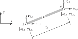
where, in accordance with Figure 2, $x_{i,e}$ and $y_{i,e}$ denote the coordinates of the $e$-th element’s nodes, $u_{i,e}$ and $v_{i,e}$ are the corresponding displacements, $\ell_{e}$ is the element length, $E_{e}$ stands for the Young’s modulus, possibly randomized in a binary sense, and $A_{e}$ for the cross-section area. The associated generalized element strain ${\boldsymbol{e}}_{e}$ and stress ${\boldsymbol{s}}_{e}$ are defined as the bar’s elongation $\Delta\ell_{e}$ and the axial force $S_{e}$, respectively.

Figure 2: Definition of the geometry and kinematics of a truss element.

Assuming that $E^{(1)}_{e}\geq E^{(2)}_{e}$ for $e=1,2,\ldots,{N_{e}}$, we introduce a dimensionless parameter in the form

$$\zeta_{\stackrel{{\scriptstyle\pm}}{{\sim}}}({\boldsymbol{P}}^{(11)})=\frac{{\mathcal{H}}_{\stackrel{{\scriptstyle\pm}}{{\sim}}}({\boldsymbol{P}}^{(11)})-H^{(2)}}{H^{(1)}-H^{(2)}}, 0\leq\zeta\leq 1,$$ (54)

to aid the visualization of results. The value of $\zeta_{\stackrel{{\scriptstyle\pm}}{{\sim}}}$ indicates the relative difference between the estimated mean energy of a random system described by the ${\boldsymbol{P}}^{(11)}$ statistics and of deterministic structures, which solely consists of states $r=1$ or $r=2$, yielding the deterministic energies $H^{(1)}$ or $H^{(2)}$.

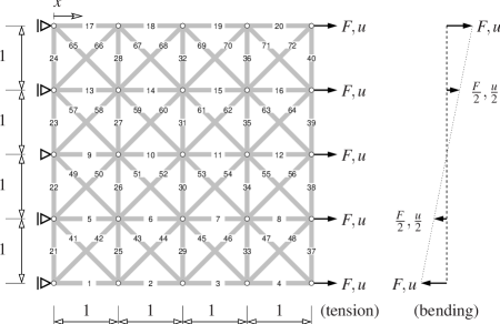
The regular lattice structure appearing in Figure 3 is employed as a benchmark problem. The prescribed boundary conditions include uniform tension and bending scenarios, imposed either using nodal forces (force control, $\mathrm{FC}$) or by prescribed nodal displacements (displacement control, $\mathrm{DC}$).

Figure 3: Sketch of the lattice structure used as a benchmark problem.

The results for second-order bounds presented hereafter are accompanied by the statistically local counterparts of the Voigt and Reuss type, determined for a deterministic problem with spatially variable Young’s moduli in the form

$$E^{\mathrm{V}}_{e}(p^{(1)}_{e}) = p^{(1)}_{e}E_{e}^{(1)}+(1-p^{(1)}_{e})E_{e}^{(2)},$$ (55)

$$E^{\mathrm{R}}_{e}(p^{(1)}_{e}) = \left(\frac{p^{(1)}_{e}}{E_{e}^{(1)}}+\frac{1-p^{(1)}_{e}}{E_{e}^{(2)}}\right)^{-1}.$$ (56)

Finally, ensemble averages obtained by direct Monte-Carlo ($\mathrm{MC}$) simulations with $N=10,000$ realizations are included as a reference.

4.1 Structure with independent elements

To demonstrate the performance of the non-local energetic bounds and estimates, we start with the analysis of the simplest stochastic system with a closed-form expression for the two-unit statistics. To this end, consider a binary structure with the first phase assigned to each element independently with a probability $\phi$. The associated second-order statistics are

$$P^{(11)}_{ee^{\prime}}=\left\{\begin{array}[]{cl}\phi&\mbox{if }e=e^{\prime},\\ \phi^{2}&\mbox{otherwise},\end{array}\right.$$ (57)

the system is therefore statistically uniform in the sense of (20). Notice that for the particular network shown in Figure 3, the cardinality of the ensemble space is $|{\mathbb{S}}|=2^{72}\doteq 4.72\cdot 10^{21}$, whereas the computable two-unit statistical characterization involves $\frac{72+1}{2}\cdot 72=2,628$ independent parameters only.

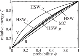
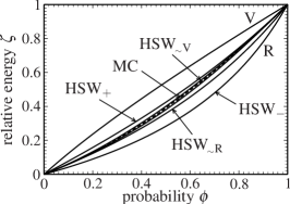
The contrast of phase stiffnesses is set to $E^{(1)}:E^{(2)}=10:1$; the most restrictive upper Hashin-Shtrikman-Willis bound ($\mathrm{HSW}_{+}$) therefore corresponds to a structure with $E^{(0)}_{e}=E^{(1)}$ and the optimal lower bound $\mathrm{HSW}_{-}$ is obtained by setting $E^{(0)}_{e}=E^{(2)}$. In addition, we include variational estimates corresponding to the reference structure with the generalized stiffness set to the Voigt upper bound ($\mathrm{HSW}_{\sim\mathrm{V}}$) or the the Reuss bound ($\mathrm{HSW}_{\sim\mathrm{R}}$).

(a) tension, $\mathrm{FC}$

(b) tension, $\mathrm{DC}$

(c) bending, $\mathrm{FC}$

(d) bending, $\mathrm{DC}$

Figure 4: Energetics of the random truss structure with independent elements; (a)–(b) tension, (c)–(d) bending. The upper ($\mathrm{HSW}_{+}$) and lower ($\mathrm{HSW}_{-}$) Hashin-Shtrikman-Willis bounds are compared with the first-order Voigt ($\mathrm{V}$) and Reuss ($\mathrm{R}$) counterparts, variational estimates for the reference structure corresponding to the Voigt ($\mathrm{HSW}_{\sim\mathrm{V}}$) and the Reuss ($\mathrm{HSW}_{\sim\mathrm{R}}$) bound and direct $\mathrm{MC}$ simulations under displacement ($\mathrm{DC}$) and force ($\mathrm{FC}$) controlled loading.

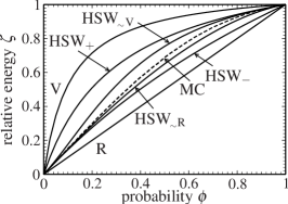
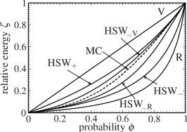
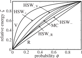
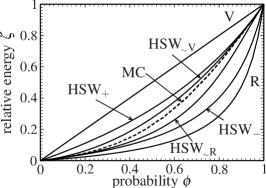
Figure 4 presents the relative energies as a function of $\phi$ for all considered loading scenarios. The $\mathrm{MC}$ curves correspond to $99\%$ confidence intervals, thereby indicating that a sufficient number of simulations was used to obtain reliable reference data. Observe that, due to the adopted dimensionless representation, the shape of the resulting curves is almost independent of the loading mode (tension or bending). For all simulations, the $\mathrm{HSW}$ bounds substantially narrow the domain defined by the first-order Voigt ($\mathrm{V})$ and Reuss ($\mathrm{R}$) bounds while preserving the concave/convex dependence of the mean potential energy on the $\phi$ parameter for the displacement- or force-driven loads, respectively. The increase in accuracy as a result of considering non-local spatial statistics is especially pronounced for small and large values of $\phi$, for which even the asymptotic behavior seems to be exactly reproduced by the lower bound for the force-controlled conditions and the upper bound in the kinematically constrained case. This observation is in an agreement with analogous results for the Hashin-Shtrikman bounds for small values of the volume fractions reported for isotropic elasticity (Roscoe, 1973) or scalar problems (Milton and Nesi, 1999). Even better agreement between the $\mathrm{HSW}$ predictions and $\mathrm{MC}$ simulations can be reached by employing the variational estimates generated by setting the reference stiffness matrix equal to the first-order bounds. Observe that for the particular system and loading conditions considered here, the $\mathrm{HSW}_{\sim\mathrm{R}}$ and $\mathrm{HSW}_{\sim\mathrm{V}}$ estimates effectively bound the reference data from above and below. As we are currently unable to establish optimality of the $\mathrm{HSW}_{+}$ and $\mathrm{HSW}_{-}$ bounds, further generalization of this fact remains an open question.

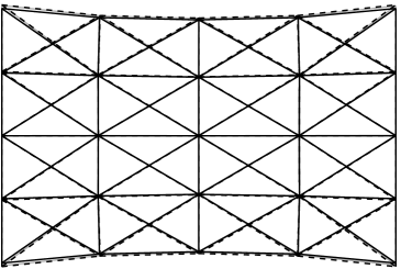
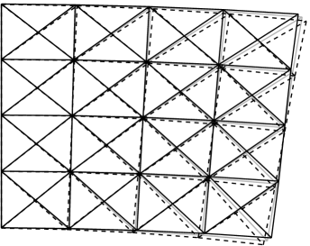
The “energetic” displacements (48) as predicted by the $\mathrm{HSW}$ bounds appear in Figure 5. For both the displacement and force driven cases, the average deformed shapes are well reproduced by the bounds with, for example, the upper energetic bound corresponding to smaller displacement values. This is fully consistent with the fact that the upper bound represents the stiffest response for a given load and two-unit statistics. Moreover, the results comply with the intuitive trend suggesting a smaller displacement range for a larger number of kinematic constraints.

(a) $\mathrm{DC}$, maximum displacement scaled to $2$ m.

(b) $\mathrm{FC}$, maximum displacement scaled to $0.25$ m.

Figure 5: Deformed structures; (a) tension, $\phi=0.3$, (b) bending, $\phi=0.6$ subject to displacement ($\mathrm{DC})$ and force ($\mathrm{FC}$) driven loading; displacements corresponding to lower/upper bound are indicated by dashed/full lines and the results of Monte-Carlo simulations are depicted in gray.

4.2 Structure with spatially variable stiffness distribution

Having demonstrated the accuracy and limitations of the bounds and estimates for a system with independent units, we focus in the second example on the effects of phase contrast and spatially variable distribution of material properties. For simplicity, the statistical model is chosen to be identical to the one introduced in the previous section; whereas the Young’s moduli of individual elements are now assumed in the form

$$\frac{E_{e}^{(1)}}{E_{e}^{(2)}}=1+\left(\rho-1\right)\frac{x_{e}}{4}, e=1,2,\ldots,{N_{e}},$$ (58)

where $x_{e}=(x_{1,e}+x_{2,e})/2$ denotes the $x$-coordinate of the $e$-th element’s center, recall Figure 3, and $\rho\geq 1$ is the maximum phase contrast.

(a) $\mathrm{FC},\rho=5$

(b) $\mathrm{DC},\rho=5$

(c) $\mathrm{FC},\rho=500$

(d) $\mathrm{DC},\rho=500$

Figure 6: Energetics of the random truss structure with spatially variable stiffness distribution subject to bending; (a)–(b) phase contrast $\rho=5$, (c)–(d) phase contrast $\rho=500$. The upper ($\mathrm{HSW}_{+}$) and lower ($\mathrm{HSW}_{-}$) Hashin-Shtrikman-Willis bounds are compared with the first-order Voigt ($\mathrm{V}$) and Reuss ($\mathrm{R}$) counterparts, variational estimates for the reference structure corresponding to the Voigt ($\mathrm{HSW}_{\sim\mathrm{V}}$) and the Reuss ($\mathrm{HSW}_{\sim\mathrm{R}}$) bound and direct $\mathrm{MC}$ simulations under displacement ($\mathrm{DC}$) and force ($\mathrm{FC}$) controlled loading.

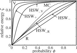
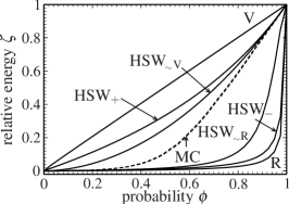
The resulting energetic bounds and estimates appear in Figure 6 for the structure subject to bending for low ($\rho=5$) and high ($\rho=500$) phase contrasts, respectively. We observe that in the low-contrast case, the region defined by the $\mathrm{HSW}_{-}$ and $\mathrm{HSW}_{+}$ bounds is substantially smaller than in the previous example, whereas the $\mathrm{HSW}_{\sim\mathrm{R}}$ and $\mathrm{HSW}_{\sim\mathrm{V}}$ estimates almost coincide with the $\mathrm{MC}$ simulation data. For increasing values of $\rho$, the accuracy of the bounds and estimates deteriorates; still the statistically non-local quantities provide an improvement over the first-order approaches. Moreover, analogously to Section 4.1, they correctly reproduce the asymptotic behavior for $\phi\rightarrow 0$ and $\phi\rightarrow 1$.

4.3 Energetics of a weakest link fracture model

In the last example, we study the ability of the bounds and estimates to capture the energetics of a simple randomized discrete fracture model with two-unit probability matrices following from computer-generated data.

In the deterministic setting, following Francfort and Marigo (1993), a damaged lattice is understood as a two-state system with a “healthy” state ($\chi_{e}^{(1)}=1,\chi_{e}^{(2)}=0$) and a fully-damaged state ($\chi_{e}^{(1)}=0,\chi_{e}^{(2)}=1$). As the fully damaged elements cannot sustain any stress, we have $E^{(2)}:E^{(1)}=0$. The transition from state $1$ to state $2$ occurs when

$$H_{e}=\mbox{$\frac{1}{2}$}{\boldsymbol{d}}_{e}{{}^{\sf T}}{\boldsymbol{K}}_{e}{\boldsymbol{d}}_{e}\geq\kappa_{e},$$ (59)

where ${\boldsymbol{K}}_{e}={\boldsymbol{B}}_{e}^{\mathsf{T}}{\boldsymbol{D}}_{e}{\boldsymbol{B}}_{e}$ and $\kappa_{e}$ denote the stiffness matrix and an energy threshold of the $e$-th element, respectively.

1. Input: probability distribution of thresholds $\kappa_{e}$ for $e=1,2,\ldots,{N_{e}}$, loading scenario $f(t)\overline{{\boldsymbol{d}}}$ with $f(0)=0,f(1)=1$ and $f$ being monotonic, number of realizations $N$ and sampling times $0=\tau_{0}<\tau_{1}<\ldots<\tau_{M}=1$

2. For $i=1,2,\ldots,N$

   1. initialize ${\boldsymbol{\phi}}=\emptyset$, ${\boldsymbol{\tau}}=\emptyset$ and ${\boldsymbol{\chi}}^{[i]}(\tau_{k})={\boldsymbol{1}}\in\mathbb{R}^{N_{e}}$ for $k=1,2,\ldots M$

   2. set $E_{e}=E$ and generate thresholds $\kappa_{e}$ for $e=1,2,\ldots,{N_{e}}$

   3. Repeat

      1. set ${}^{{\boldsymbol{\phi}}}{\boldsymbol{\chi}}^{[i]}(\tau_{k})={\boldsymbol{0}}$ and $E_{e}=0$ for $e\in{\boldsymbol{\phi}}$ and $j\in{\boldsymbol{\tau}}$

      2. for current values of $E_{e}$, compute element energies $\overline{H}_{e}$ (59) using displacements ${\boldsymbol{d}}_{e}$ determined from (8) with ${}^{{\boldsymbol{c}}}{\boldsymbol{d}}=\overline{{\boldsymbol{d}}}$; $e=1,2,\ldots,{N_{e}}$

      3. set ${\boldsymbol{\varepsilon}}=\{e=1,2,\ldots,{N_{e}}:\overline{H}_{e}>0\}$

      4. compute $t_{e}=f^{-1}\left(\sqrt{\kappa_{e}^{[i]}/\overline{H}_{e}}\right)$ for $e\in{\boldsymbol{\varepsilon}}$

      5. set $t=\min_{e\in{\boldsymbol{\varepsilon}}}\{t_{e}\}$

      6. set ${\boldsymbol{\phi}}=\left\{e\in{\boldsymbol{\varepsilon}}:t_{e}=t\right\}$

      7. set ${\boldsymbol{\tau}}=\left\{k=1,2,\ldots,M:\tau_{k}\geq t\right\}$

      until $t>1$ or ${\boldsymbol{\varepsilon}}=\emptyset$

3. using samples $\{{\boldsymbol{\chi}}^{[i]}(\tau_{k}){{\boldsymbol{\chi}}^{[i]}}{{}^{\sf T}}(\tau_{k})\}_{i=1}^{N}$, compute ${\boldsymbol{P}}_{\mathrm{MC}}^{(11)}(\tau_{k})$ for $k=1,2,\ldots,M$

4. using samples $\{H^{[i]}(\tau_{k})\}_{i=1}^{N}$, compute ${\mathcal{H}}^{\mathrm{MC}}(\tau_{k})$ for $k=1,2,\ldots,M$, where $H^{[i]}(\tau_{k})=\sum_{e=1}^{N_{e}}H_{e}$, with $H_{e}$ provided by (59) using displacements ${\boldsymbol{d}}_{e}$ determined from (8) with ${}^{{\boldsymbol{c}}}{\boldsymbol{d}}=f(\tau_{k})\overline{{\boldsymbol{d}}}$ and $E_{e}=\chi^{[i]}_{e}(\tau_{k})E$

Table 1: Conceptual implementation of the weakest link algorithm.

The stochastic damage evolution is simulated using a simple combination of an “event-by-event” strategy and a direct Monte-Carlo algorithm as outlined in Table 1. For every realization of energy thresholds, a deterministic time-stepping procedure is executed. First, the structure is subjected to the full displacements and the energies corresponding to individual elements are extracted (step ii.). Then, in steps iii.–vii., the element(s) with the highest damage affinity is (are) determined and removed from the structure (step i.). This is accompanied by the bookkeeping of element deactivation times in terms of the auxiliary matrices ${\boldsymbol{\chi}}^{[i]}(\tau_{k}),k=1,2,\ldots,M$. The procedure is repeated until the imposed loading sequence is completed or until the structure loses its integrity; cf. the termination conditions of step (c). After the sampling phase is complete, quantities of interest related to the damage statistics follow from post-processing of the simulation results (steps 3. and 4.); see also e.g. (Sharif-Khodaei and Zeman, 2008; Alava et al., 2006; Vellinga et al., 2008) and references therein for more details.

In particular, we consider the lattice shown in Figure 3 subject to an imposed displacement, which is parametrized as

$$u(t)=u_{\max}\sqrt{t},\quad 0\leq t\leq 1,$$ (60)

leading to a linear scaling of the element energies (59) with respect to the pseudo-time $t$.

For simplicity, identical values of the Young’s moduli, $E^{(1)}_{e}=E$, are assumed in the healthy state for every element and the thresholds are taken as uniformly distributed independent random variables ranging from $\kappa_{e}^{-}=\frac{1}{4}E_{e}A_{e}(\Delta\ell_{e}^{\mathrm{cr}})^{2}/\ell_{e}$ to $\kappa_{e}^{+}=3\kappa_{e}^{-}$ with the critical elongation $\Delta\ell_{e}^{\mathrm{cr}}=10^{-3}\ell_{e}$. The target displacement is set to $u_{\max}=10^{-2}$ for uniform tension, whereas for the bending case $u_{\max}=1.5\cdot 10^{-2}$. The time evolution of the system was sampled at $M=100$ uniformly distributed time instants using $N=10,000$ realizations.

Figure 7: Evolution of the one- and two-unit probability matrix ${\boldsymbol{P}}_{\mathrm{MC}}^{(11)}$ entries as determined by Monte-Carlo simulations. The snapshots for $t=0.1$ and $t=0.6$ show one-unit probabilities, whereas complete two-unit probability matrix is plotted for $t=0.9$.

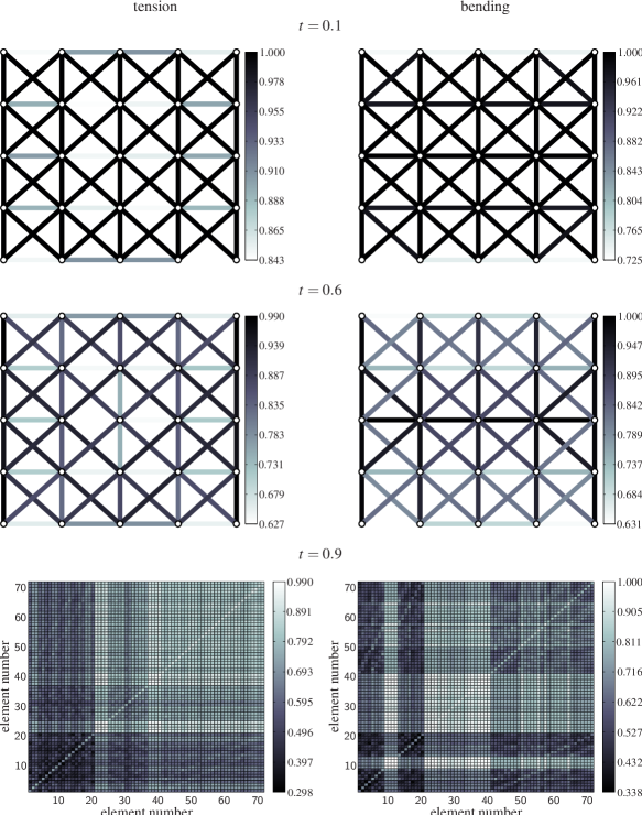
Snapshots of the damage progress quantified in terms of one- and two-unit probabilities appear in Figure 7 for both the uniform tension and bending scenarios. Note that the diagonal entries of the ${\boldsymbol{P}}^{(11)}(t)$ matrix provide, in the current setting, the survival probability for each element at time $t$. The off-diagonal values correspond to the simultaneous survival probabilities for two elements.

In the case of uniform tension, the damage distribution appears to be rather diffuse during the whole loading procedure. Low survival probabilities are localized in the horizontal links in the corners of the network and in the structure’s interior, as these exhibit the highest failure affinity for the deterministic solution with $2\kappa_{e}=\kappa_{e}^{-}+\kappa_{e}^{+}$ (pseudo-time $t=0.1)$. The slight non-symmetry of the one-unit probabilities visible in Figure 7 results from the finite number of realizations used to sample the statistics. With increasing load, the remaining horizontal elements start to fail due to the energy redistribution after failure of the first group of weakest links, leading to a decrease of the survival probabilities for the interior elements ($t=0.6$). In the case of bending, on the other hand, the damage is triggered mainly in the upper and lower rows of elements and subsequently propagates to internal links. Additional details on the simultaneous survival probabilities are given by the full two-unit probability matrices, shown in Figure 7 for $t=0.9$. Recalling element numbering introduced in Figure 3, the plots reveal, among other things, simultaneous survival probabilities close to one for vertical element groups $21$–$24$ and $37$–$40$, which connects the nodes where the load is imposed, and horizontal elements $9$–$10$, at the neutral axis, in the case of bending. It follows from these results that the second-order statistics correctly capture the dominant fracture mechanisms, thereby providing a well-founded statistically non-local damage parameter for stochastic damage theories.

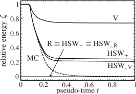
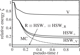
The evolution of the normalized stored energy $\zeta$ is depicted in Figure 8. The choice of reference structures to generate the bounds or estimates is identical to that in the previous example. Note that the lower bounds and the $\mathrm{HSW}_{\sim\mathrm{R}}$ estimate are identically equal to zero due to the zero stiffness assigned to the weaker state. The overall character of the energy evolution is consistent with the previous discussion. In particular, two failure modes are clearly visible for the bending problem, whereas the gradual decrease in energy for uniform tension corresponds to more a diffuse damage character. Similarly to Section 4.1, the first-order Voigt bounds correctly predict the trend of the energy reduction, but under predicts its magnitude. The $\mathrm{HSW}$ bound remains highly accurate until $t\approx 0.2$. A certain discrepancy, however, is observed for the limit value of the dimensionless energy, e.g. $\zeta^{\mathrm{HSW}_{+}}\doteq 0.24$ instead of the reference $\zeta^{\mathrm{MC}}\approx 0$ for uniform tension, cf. Figure 8(a). This difference again arises due to the fact that the upper $\mathrm{HSW}$ bound corresponds, in the ensemble average sense, to the response of the stiffest structure compatible with the two-unit statistics shown in Figure 7, for which the minimum probability reaches $\approx 30\%$ for both loading sequences. The results of the $\mathrm{MC}$ simulations, on the other hand, represent one particular stochastic system implicitly defined by the randomization procedure and the event-by-event solution algorithm. Nevertheless, the added value of the second-order relations becomes apparent when considering the Voigt prediction $\zeta^{\mathrm{V}}\doteq 0.74$. Slightly more accurate values of the residual relative energy can be generated using the $\mathrm{HSW}_{\sim\mathrm{V}}$ estimate, for which we obtain $\zeta^{\mathrm{HSW}_{\sim\mathrm{V}}}\doteq 0.21$. The general character of these conclusions is further supported by the analogous results of the bending mode shown in Figure 8(b).

Figure 8: Energetics of the weakest link model; (a) tension, (b) bending.

5 Conclusions

In this work, variational bounds and estimates of the Hashin-Shtrikman-Willis ($\mathrm{HSW}$) type for two-phase random structures have been derived and verified against the results of direct Monte-Carlo ($\mathrm{MC}$) simulations. The most important findings can be summarized as follows:

• When applied to discrete structures instead of continua, the derivation of the $\mathrm{HSW}$ principles becomes reasonably straightforward and requires only elements of matrix structural analysis and linear algebra.

• The variational framework naturally incorporates general statistically non-uniform systems, including the specification of the set of all admissible two-unit probability matrices. Thus, the developed statistically non-local theory is able to treat the statistics of systems with independent and highly correlated units in a unified manner.

• The second-order bounds and estimates provide a computationally feasible alternative to direct $\mathrm{MC}$ simulations.

• When applied to the displacement-driven damage problems, the upper bound on the stored energy delivers a reasonably accurate approximation to the total potential energy at the damage initiation and propagation without any adjustable parameters. When complemented with an accurate representation of the irreversible energy dissipation during the damage process, the scheme has the potential to provide a consistent variational model for damage evolution in discrete media.

The developed statistically non-local discrete theory can also provide a convenient starting point for the coarsening towards an equivalent continuum representation. The already announced applications, i.e. a variational approach to deterministic and stochastic damage mechanics of finite-sized lattices and incorporation of higher-order statistics, will explored and reported separately in future publications.

Appendix A Derivation of condensed energy

Recall that the expression for the condensed energy follows from the value of the Hashin-Shtrikman function (34) with the displacement vector optimally adjusted to a trial generalized polarization stress $\widehat{{\boldsymbol{\tau}}}$. In particular, evaluating the energy for the displacement ${}^{{\boldsymbol{u}}}\tilde{{\boldsymbol{d}}}$ determined from (36) yields, in a partitioned format:

$$U({}^{{\boldsymbol{u}}}\tilde{{\boldsymbol{d}}},\widehat{{\boldsymbol{\tau}}};\alpha) = \mbox{$\frac{1}{2}$}\left[\begin{array}[]{c}{}^{{\boldsymbol{u}}}{\boldsymbol{d}}{{}_{(0)}}+{}^{{\boldsymbol{u}}}\tilde{{\boldsymbol{d}}}{{}_{(1)}}\\ {}^{{\boldsymbol{c}}}{\boldsymbol{d}}\end{array}\right]^{\sf T}\left[\begin{array}[]{cc}{}^{{\boldsymbol{u}}{\boldsymbol{u}}}{\boldsymbol{K}}^{(0)}&{}^{{\boldsymbol{u}}{\boldsymbol{c}}}{\boldsymbol{K}}^{(0)}\\ {}^{{\boldsymbol{c}}{\boldsymbol{u}}}{\boldsymbol{K}}^{(0)}&{}^{{\boldsymbol{c}}{\boldsymbol{c}}}{\boldsymbol{K}}^{(0)}\end{array}\right]\left[\begin{array}[]{c}{}^{{\boldsymbol{u}}}{\boldsymbol{d}}{{}_{(0)}}+{}^{{\boldsymbol{u}}}\tilde{{\boldsymbol{d}}}{{}_{(1)}}\\ {}^{{\boldsymbol{c}}}{\boldsymbol{d}}\end{array}\right]$$

$$- \left({}^{{\boldsymbol{u}}}{\boldsymbol{d}}{{}_{(0)}}+{}^{{\boldsymbol{u}}}\tilde{{\boldsymbol{d}}}{{}_{(1)}}\right){{}^{\sf T}}~{}{}^{{\boldsymbol{u}}}{\boldsymbol{f}}+\widehat{{\boldsymbol{\tau}}}{{}^{\sf T}}\left[\begin{array}[]{cc}{}^{:{\boldsymbol{u}}}{\boldsymbol{B}}&{}^{:{\boldsymbol{c}}}{\boldsymbol{B}}\end{array}\right]\left[\begin{array}[]{c}{}^{{\boldsymbol{u}}}{\boldsymbol{d}}{{}_{(0)}}+{}^{{\boldsymbol{u}}}\tilde{{\boldsymbol{d}}}{{}_{(1)}}\\ {}^{{\boldsymbol{c}}}{\boldsymbol{d}}\end{array}\right]$$

$$+ \mbox{$\frac{1}{2}$}\widehat{{\boldsymbol{\tau}}}\left({\boldsymbol{D}}^{(0)}-{\boldsymbol{D}}(\alpha)\right)^{-1}\widehat{{\boldsymbol{\tau}}}.$$

A suitable re-arrangement of terms appearing in the previous relation together with the optimality conditions (37) and (38) leads to

$$U({}^{{\boldsymbol{u}}}\tilde{{\boldsymbol{d}}},\widehat{{\boldsymbol{\tau}}};\alpha) = \overbrace{\mbox{$\frac{1}{2}$}\left[\begin{array}[]{c}{}^{{\boldsymbol{u}}}{\boldsymbol{d}}{{}_{(0)}}\\ {}^{{\boldsymbol{c}}}{\boldsymbol{d}}\end{array}\right]^{\sf T}\left[\begin{array}[]{cc}{}^{{\boldsymbol{u}}{\boldsymbol{u}}}{\boldsymbol{K}}^{(0)}&{}^{{\boldsymbol{u}}{\boldsymbol{c}}}{\boldsymbol{K}}^{(0)}\\ {}^{{\boldsymbol{c}}{\boldsymbol{u}}}{\boldsymbol{K}}^{(0)}&{}^{{\boldsymbol{c}}{\boldsymbol{c}}}{\boldsymbol{K}}^{(0)}\end{array}\right]\left[\begin{array}[]{c}{}^{{\boldsymbol{u}}}{\boldsymbol{d}}{{}_{(0)}}\\ {}^{{\boldsymbol{c}}}{\boldsymbol{d}}\end{array}\right]-{}^{{\boldsymbol{u}}}{\boldsymbol{d}}{{}_{(0)}}{{}^{\sf T}}{}^{{\boldsymbol{u}}}{\boldsymbol{f}}}^{=H^{(0)}\text{~{}by definition}}$$

$$+ \widehat{{\boldsymbol{\tau}}}{{}^{\sf T}}\overbrace{\left[\begin{array}[]{cc}{}^{:{\boldsymbol{u}}}{\boldsymbol{B}}&{}^{:{\boldsymbol{c}}}{\boldsymbol{B}}\end{array}\right]\left[\begin{array}[]{c}{}^{{\boldsymbol{u}}}{\boldsymbol{d}}{{}_{(0)}}\\ {}^{{\boldsymbol{c}}}{\boldsymbol{d}}\end{array}\right]}^{={\boldsymbol{e}}{{}_{(0)}}\text{~{}by definition}}+\mbox{$\frac{1}{2}$}\widehat{{\boldsymbol{\tau}}}\left({\boldsymbol{D}}^{(0)}-{\boldsymbol{D}}(\alpha)\right)^{-1}\widehat{{\boldsymbol{\tau}}}$$

$$+ \mbox{$\frac{1}{2}$}\widehat{{\boldsymbol{\tau}}}{{}^{\sf T}}\overbrace{{}^{:{\boldsymbol{u}}}{\boldsymbol{B}}\,{}^{{\boldsymbol{u}}}\tilde{{\boldsymbol{d}}}{{}_{(1)}}}^{=-{\boldsymbol{\Gamma}}^{(0)}\widehat{{\boldsymbol{\tau}}}\text{~{}by~{}Eq.~{}(\ref{eq:gamma_0_def})}}+\mbox{$\frac{1}{2}$}{}^{{\boldsymbol{u}}}\tilde{{\boldsymbol{d}}}{{}_{(1)}}{{}^{\sf T}}\overbrace{\left({\boldsymbol{K}}^{(0)}{}^{{\boldsymbol{u}}}\tilde{{\boldsymbol{d}}}{{}_{(1)}}+{}^{:{\boldsymbol{u}}}{\boldsymbol{B}}{{}^{\sf T}}\widehat{{\boldsymbol{\tau}}}\right)}^{={\boldsymbol{0}}\text{~{}by Eq.~{}(\ref{eq:system_2})}}$$

$$+ {}^{{\boldsymbol{u}}}\tilde{{\boldsymbol{d}}}{{}_{(1)}}{{}^{\sf T}}\overbrace{\left(\left[\begin{array}[]{cc}{}^{{\boldsymbol{u}}{\boldsymbol{u}}}{\boldsymbol{K}}^{(0)}&{}^{{\boldsymbol{u}}{\boldsymbol{c}}}{\boldsymbol{K}}^{(0)}\end{array}\right]\left[\begin{array}[]{c}{}^{{\boldsymbol{u}}}{\boldsymbol{d}}{{}_{(0)}}\\ {}^{{\boldsymbol{c}}}{\boldsymbol{d}}\end{array}\right]-{}^{{\boldsymbol{u}}}{\boldsymbol{f}}\right)}^{={\boldsymbol{0}}\text{~{}by Eq.~{}(\ref{eq:system_1})}}$$

which coincides with the expression for the condensed energy as appearing in Eq. (40). Note that similar development for the continuous case is available in, e.g., Willis (1977) and in Willis (1981), with the FE-discretization treated in Luciano and Willis (2005).

References

- Alava et al. (2006) Alava, M. J., Nukala, P. K. V. V., Zapperi, S., 2006. Statistical models of fracture. Advances in Physics 55 (3–4), 349–476.
- Alicandro and Cicalese (2005) Alicandro, R., Cicalese, M., 2005. A general integral representation result for continuum limits of discrete energies with superlinear growth. SIAM Journal of Mathematical Analysis 36 (1), 1–37.
- Alicandro et al. (2007) Alicandro, R., Cicalese, M., Gloria, A., 2007. Mathematical derivation of a rubber-like stored energy functional. Comptes Rendus Mathématique 345 (8), 479–482.
- Alicandro et al. (2010) Alicandro, R., Cicalese, M., Gloria, A., 2010. Integral representation results for energies defined on stochastic lattices and application to nonlinear elasticity. Archive for Rational Mechanics and Analysis, accepted for publication. http://cvgmt.sns.it/cgi/get.cgi/papers/alicicglo09
- Arndt and Griebel (2005) Arndt, M., Griebel, M., 2005. Derivation of higher order gradient continuum models from atomistic models for crystalline solids. Multiscale Modeling and Simulation 4 (2), 531–562.
- Arnoux et al. (2002) Arnoux, P. J., Bonnoit, J., Chabrand, P., Jean, M., Pithioux, M., 2002. Numerical damage models using a structural approach: Application in bones and ligaments. EPJ Applied Physics 17 (1), 65–73.
- Bardenhagen and Triantafyllidis (1994) Bardenhagen, S., Triantafyllidis, N., 1994. Derivation of higher order gradient continuum theories in 2,3-D non-linear elasticity from periodic lattice models. Journal of the Mechanics and Physics of Solids 42 (1), 111–139.
- Bažant and Jirásek (2002) Bažant, Z. P., Jirásek, M., 2002. Nonlocal integral formulations of plasticity and damage: Survey of progress. Journal of Engineering Mechanics 128 (11), 1119–1149.
- Berezhnyy and Berlyand (2006) Berezhnyy, M., Berlyand, L., 2006. Continuum limit for three-dimensional mass-spring networks and discrete Korn’s inequality. Journal of the Mechanics and Physics of Solids 54 (3), 635–669.
- Blanc et al. (2005) Blanc, X., Le Bris, C., Legoll, F., 2005. Analysis of a prototypical multiscale method coupling atomistic and continuum mechanics. Mathematical Modelling and Numerical Analysis 39 (4), 797–826.
- Blanc et al. (2002) Blanc, X., Le Bris, C., Lions, P.-L., 2002. From molecular models to continuum mechanics. Archive for Rational Mechanics and Analysis 164 (4), 341–381.
- Blanc et al. (2007a) Blanc, X., Le Bris, C., Lions, P.-L., 2007a. Atomistic to continuum limits for computational materials science. Mathematical Modelling and Numerical Analysis 41 (2), 391–426.
- Blanc et al. (2007b) Blanc, X., Le Bris, C., Lions, P.-L., 2007b. The energy of some microscopic stochastic lattices. Archive for Rational Mechanics and Analysis 184 (2), 303–339.
- Blanc et al. (2007c) Blanc, X., Le Bris, C., Lions, P.-L., 2007c. Stochastic homogenization and random lattices. Journal de Mathématiques Pures et Appliqués 88 (1), 34–63.
- Bouchitté et al. (2009) Bouchitté, G., Mielke, A., Roubíček, T., 2009. A complete-damage problem at small strains. Zeitschrift für Angewandte Mathematik und Physik (ZAMP) 60 (2), 205–236.
- Braides and Francfort (2004) Braides, A., Francfort, G. A., 2004. Bounds on the effective behaviour of a square conducting lattice. Proceedings of the Royal Society A: Mathematical, Physical and Engineering Sciences 460 (2046), 1755–1769.
- Braides and Gelli (2002) Braides, A., Gelli, M. S., 2002. Continuum limits of discrete systems without convexity hypotheses. Mathematics and Mechanics of Solids 7 (1), 41–66.
- Braides and Piatnitski (2008) Braides, A., Piatnitski, A., 2008. Overall properties of a discrete membrane with randomly distributed defects. Archive for Rational Mechanics and Analysis 189 (2), 301–323.
- Bronkhorst (2003) Bronkhorst, C. A., 2003. Modelling paper as a two-dimensional elastic-plastic stochastic network. International Journal of Solids and Structures 40 (20), 5441–5454.
- Christensen (2000) Christensen, R. M., 2000. Mechanics of cellular and other low-density materials. International Journal of Solids and Structures 37 (1–2), 93–104.
- Chudoba et al. (2006) Chudoba, R., Vořechovský, M., Konrad, M., 2006. Stochastic modeling of multi-filament yarns. I. Random properties within the cross-section and size effect. International Journal of Solids and Structures 43 (3–4), 413–434.
- Cusatis et al. (2006) Cusatis, G., Bažant, Z. P., Cedolin, L., 2006. Confinement-shear lattice CSL model for fracture propagation in concrete. Computer Methods in Applied Mechanics and Engineering 195 (52), 7154–7171.
- Dvorak and Srinivas (1999) Dvorak, G. J., Srinivas, M. V., 1999. New estimates of overall properties of heterogeneous solids. Journal of the Mechanics and Physics of Solids 47 (4), 899–920.
- Eringen (2002) Eringen, C., 2002. Nonlocal Continuum Field Theories. Springer Verlag, New York, USA.
- Francfort and Marigo (1993) Francfort, G., Marigo, J., 1993. Stable damage evolution in a brittle continuous medium. European Journal of Mechanics A-Solids 12 (2), 149–189.
- Friesecke and Theil (2002) Friesecke, G., Theil, F., 2002. Validity and failure of the Cauchy-Born hypothesis in a two-dimensional mass-spring lattice. Journal of Nonlinear Science 12 (5), 445–478.
- Ganghoffer et al. (1999) Ganghoffer, J. F., Sluys, L. J., De Borst, R., 1999. A reappraisal of nonlocal mechanics. European Journal of Mechanics, A/Solids 18 (1), 17–46.
- Gavinia et al. (2007) Gavinia, V., Bhattacharya, K., Ortiz, M., 2007. Quasi-continuum orbital-free density-functional theory: A route to multi-million atom non-periodic DFT calculation. Journal of the Mechanics and Physics of Solids 55 (4), 669–696.
- Grassl and Jirásek (2010) Grassl, P., Jirásek, M., 2010. Meso-scale approach to modelling the fracture process zone of concrete subjected to uniaxial tension. International Journal of Solids and Structures 47 (7–8), 957–968.
- Hashin and Shtrikman (1962) Hashin, Z., Shtrikman, S., 1962. On some variational principles in anisotropic and nonhomogeneous elasticity. Journal of the Mechanics and Physics of Solids 10, 335–342.
- Horn and Johnson (1990) Horn, R., Johnson, C., 1990. Matrix Analysis. Cambridge University Press.
- Ibrahimbegovic and Delaplace (2003) Ibrahimbegovic, A., Delaplace, A., 2003. Microscale and mesoscale discrete models for dynamic fracture of structures built of brittle material. Computers and Structures 81 (12), 1255–1265.
- Iosifescu et al. (2001) Iosifescu, O., Licht, C., Michaille, G., 2001. Variational limit of a one dimensional discrete and statistically homogeneous system of material points. Asymptotic Analysis 28 (3–4), 309–329.
- Jagla (2007) Jagla, E. A., 2007. Modeling the buckling and delamination of thin films. Physical Review B - Condensed Matter and Materials Physics 75 (8), article number 085405.
- Jiao et al. (2007) Jiao, Y., Stillinger, F. H., Torquato, S., 2007. Modeling heterogeneous materials via two-point correlation functions: Basic principles. Physical Review E - Statistical, Nonlinear, and Soft Matter Physics 76 (3), article number 031110.
- Jirásek and Bažant (2001) Jirásek, M., Bažant, Z. P., 2001. Inelastic Analysis of Structures. John Wiley & Sons.
- Lilliu and van Mier (2003) Lilliu, G., van Mier, J. G. M., 2003. 3D lattice type fracture model for concrete. Engineering Fracture Mechanics 70 (7–8), 927–941.
- Luciano and Willis (2005) Luciano, R., Willis, J. R., 2005. FE analysis of stress and strain fields in finite random composite bodies. Journal of the Mechanics and Physics of Solids 53 (7), 1505–1522.
- Luciano and Willis (2006) Luciano, R., Willis, J. R., 2006. Hashin-Shtrikman based FE analysis of the elastic behaviour of finite random composite bodies. International Journal of Fracture 137 (1–4), 261–273.
- Martinsson and Babuška (2007) Martinsson, P. G., Babuška, I., 2007. Homogenization of materials with periodic truss or frame micro-structures. Mathematical Models and Methods in Applied Sciences 17 (5), 805–832.
- Miehe and Dettmar (2004) Miehe, C., Dettmar, J., 2004. A framework for micro-macro transitions in periodic particle aggregates of granular materials. Computer Methods in Applied Mechanics and Engineering 193 (3–5), 225–256.
- Mielke (2009) Mielke, A., 2009. Complete-damage evolution based on energies and stresses. Discrete and Continuous Dynamical Systems Series S, accepted for publication (WIAS Preprint 1414).
- Mielke et al. (2010) Mielke, A., Roubíček, T., Zeman, J., 2010. Complete damage in elastic and viscoelastic media and its energetics. Computer Methods in Applied Mechanics and Engineering 199 (21–22), 1242–1253.
- Miller and Tadmor (2002) Miller, R. E., Tadmor, E. B., 2002. The Quasicontinuum Method: Overview, applications and current directions. Journal of Computer-Aided Materials Design 9 (3), 203–239.
- Milton and Nesi (1999) Milton, G. W., Nesi, V., 1999. Optimal -closure bounds via stability under lamination. Archive for Rational Mechanics and Analysis 150 (3), 191–207.
- Ostoja-Starzewski (2002) Ostoja-Starzewski, M., 2002. Lattice models in micromechanics. Applied Mechanics Reviews 55 (1), 35–59.
- Ostoja-Starzewski and Stahl (2001) Ostoja-Starzewski, M., Stahl, D. C., 2001. Random fiber networks and special elastic orthotropy of paper. Journal of Elasticity 60 (2), 131–149.
- Padberg (1989) Padberg, M., 1989. The Boolean quadric polytope: Some characteristics, facets and relatives. Mathematical Programming 45 (1–3), 139–172.
- Pradel and Sab (1998) Pradel, F., Sab, K., 1998. Cosserat modelling of elastic periodic lattice structures. Comptes Rendus de l’Academie de Sciences - Serie IIb: Mécanique, Physique, Chimie, Astronomie 326 (11), 699–704.
- Quintanilla (2008) Quintanilla, J. A., 2008. Necessary and sufficient conditions for the two-point phase probability function of two-phase random media. Proceedings of the Royal Society A: Mathematical, Physical and Engineering Sciences 464 (2095), 1761–1779.
- Rinaldi and Lai (2007) Rinaldi, A., Lai, Y.-C., 2007. Statistical damage theory of 2D lattices: Energetics and physical foundations of damage parameter. International Journal of Plasticity 23 (10–11), 1796–1825.
- Roscoe (1973) Roscoe, R., 1973. Isotropic composites with elastic or viscoelastic phases: General bounds for the moduli and solutions for special geometries. Rheologica Acta 12 (3), 404–411.
- Sharif-Khodaei and Zeman (2008) Sharif-Khodaei, Z., Zeman, J., 2008. Microstructure-based modeling of elastic functionally graded materials: One dimensional case. Journal of Mechanics of Materials and Structures 3 (9), 1773–1796.
- Tadmor et al. (1996) Tadmor, E. B., Ortiz, M., Phillips, R., 1996. Quasicontinuum analysis of defects in solids. Philosophical Magazine A 73 (6), 1529–1563.
- Torquato (2002) Torquato, S., 2002. Random heterogeneous materials: Microstructure and macroscopic properties. Springer-Verlag.
- Triantafyllidis and Bardenhagen (1993) Triantafyllidis, N., Bardenhagen, S., 1993. On higher order gradient continuum theories in 1-D nonlinear elasticity. Derivation from and comparison to the corresponding discrete models. Journal of Elasticity 33 (3), 259–293.
- Vellinga et al. (2008) Vellinga, W., Van den Bosch, M., Geers, M., 2008. Interaction between cracking, delamination and buckling in brittle elastic films. International Journal of Fracture 154 (1–2), 195–209.
- Vořechovský and Chudoba (2006) Vořechovský, M., Chudoba, R., 2006. Stochastic modeling of multi-filament yarns: II. Random properties over the length and size effect. International Journal of Solids and Structures 43 (3–4), 435–458.
- Willis (1977) Willis, J. R., 1977. Bounds and self-consistent estimates for the overall properties of anisotropic composites. Journal of the Mechanics and Physics of Solids 25 (3), 185–202.
- Willis (1981) Willis, J. R., 1981. Variational and related methods for the overall properties of composites. In: Advances in Applied Mechanics. Vol. 21. pp. 2–74.